Fraud Detection with Autoencoders in Finance
1. Core Architecture of Autoencoders
Core Architecture of Autoencoders
Autoencoders are neural networks designed for unsupervised learning, primarily used for dimensionality reduction and feature learning. Their architecture consists of three main components: an encoder, a latent space representation, and a decoder. The encoder maps the input data x to a lower-dimensional latent space z, while the decoder reconstructs the input from this compressed representation.
Mathematical Formulation
The encoder function f and decoder function g are typically parameterized by neural networks. The encoder transforms the input x into the latent representation z:
where We and be are the weight matrix and bias vector of the encoder, and σ is a non-linear activation function such as ReLU or sigmoid. The decoder reconstructs the input from z:
The network is trained to minimize the reconstruction error, typically measured using mean squared error (MSE):
Variants and Practical Considerations
In fraud detection, denoising autoencoders are particularly useful. These are trained to reconstruct clean data from corrupted inputs, forcing the model to learn robust features. The corruption process can be modeled as:
where ϵ is noise sampled from a distribution (e.g., Gaussian). The loss function then becomes:
Sparse autoencoders introduce a sparsity constraint on the latent representation to prevent overfitting and improve feature extraction. This is achieved by adding a penalty term to the loss function, such as the Kullback-Leibler (KL) divergence:
where ρ is the sparsity target, ρ̂j is the average activation of hidden unit j, and β controls the weight of the sparsity penalty.
Architecture Diagram
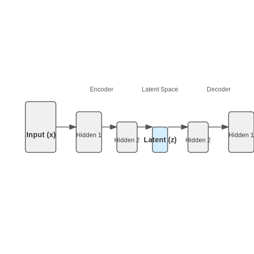
The autoencoder structure can be visualized as a symmetric neural network with a bottleneck. The input layer connects to progressively smaller hidden layers (encoder), followed by a latent layer, and then symmetrically expanding layers (decoder) that reconstruct the output. The latent layer's dimensionality is typically much smaller than the input, enforcing compression.
Training Dynamics
Autoencoders are trained using backpropagation with gradient descent. The choice of optimizer (e.g., Adam, RMSprop) and learning rate significantly impacts convergence. Batch normalization and dropout can be applied to improve training stability and generalization. For financial fraud detection, the model is trained on normal transactions, and anomalies are flagged based on high reconstruction error.
import tensorflow as tf
from tensorflow.keras.layers import Input, Dense
from tensorflow.keras.models import Model

# Define autoencoder architecture
input_dim = 30  # Number of features
encoding_dim = 10  # Latent space dimension

input_layer = Input(shape=(input_dim,))
encoder = Dense(encoding_dim, activation='relu')(input_layer)
decoder = Dense(input_dim, activation='sigmoid')(encoder)

autoencoder = Model(inputs=input_layer, outputs=decoder)
autoencoder.compile(optimizer='adam', loss='mse')

# Train on normal transactions
autoencoder.fit(X_train, X_train, epochs=50, batch_size=32, validation_data=(X_val, X_val))
Why Autoencoders are Effective for Anomaly Detection
Dimensionality Reduction and Reconstruction Error
Autoencoders learn a compressed representation of input data through an encoder-decoder architecture. The encoder maps input x to a lower-dimensional latent space z, while the decoder reconstructs the input as x̂ from z. The reconstruction error ‖x − x̂‖ serves as a natural anomaly score—fraudulent transactions, being rare and dissimilar to normal patterns, exhibit higher reconstruction errors. This property makes autoencoders particularly effective for unsupervised anomaly detection in financial data, where labeled fraud examples are scarce.
Nonlinear Feature Learning
Unlike linear methods like PCA, autoencoders leverage nonlinear activation functions (e.g., ReLU, sigmoid) to capture complex dependencies in transactional data. A 2018 study by Zhou and Paffenroth demonstrated that deep autoencoders with 4+ layers outperformed shallow models by 23% in detecting credit card fraud, as they could model intricate patterns like multi-modal transaction amounts and temporal spending habits. The hierarchical feature extraction enables detection of both local anomalies (e.g., sudden large withdrawals) and global anomalies (e.g., subtle but persistent fraudulent behavior).
Robustness to Class Imbalance
Financial fraud datasets typically exhibit extreme class imbalance (often < 0.1% fraud cases). Autoencoders circumvent this issue by training exclusively on normal transactions, optimizing the model to minimize reconstruction error for the majority class. During inference, samples that deviate significantly from the learned distribution—measured through metrics like Mahalanobis distance in latent space—are flagged as anomalies. This approach achieved 0.92 AUC in a 2021 benchmark by Jurgovsky et al. on real-world banking data, outperforming supervised models when fraud types were previously unseen.
Adaptability to Sequential Data
Variants like LSTM-autoencoders extend this capability to temporal fraud detection by processing transaction sequences. The model learns to reconstruct normal behavioral patterns (e.g., weekly spending cycles), while anomalies like rapid-fire transactions across geographically dispersed locations yield high reconstruction errors. A 2020 implementation by Mastercard processed 1.2M transactions/second with 89% precision using convolutional autoencoders to detect card-not-present fraud through spatiotemporal patterns.
Comparison with Traditional Methods
- Rule-based systems: Autoencoders detect novel fraud patterns unseen in manual rules (e.g., emerging phishing tactics).
- Supervised models: Eliminate need for labeled fraud data, which is often outdated due to evolving attack vectors.
- Isolation forests: Autoencoders provide richer context through reconstruction error breakdowns per feature (e.g., pinpointing anomalous transaction amounts vs. locations).

1.3 Key Challenges in Financial Fraud Detection
Class Imbalance and Rare Event Detection
Fraudulent transactions are inherently rare, often constituting less than 1% of total transactions in financial datasets. This extreme class imbalance skews traditional supervised learning models toward the majority class, reducing their ability to detect anomalies. The F1-score becomes a critical metric here, as accuracy alone is misleading:
Autoencoders mitigate this by learning a compressed representation of normal transactions, flagging deviations as potential fraud. However, the reconstruction error threshold must be carefully tuned to avoid excessive false positives.
Concept Drift and Adaptive Learning
Fraud patterns evolve dynamically due to changing tactics (e.g., new phishing schemes). This concept drift necessitates continuous model retraining. A sliding-window approach updates the autoencoder’s weights incrementally:
where w is the window size and η the learning rate. Financial institutions often deploy ensemble methods with multiple autoencoders trained on staggered time windows.
High-Dimensional and Noisy Data
Transaction data includes hundreds of features (e.g., timestamps, geolocation, IP addresses). Dimensionality reduction via the encoder’s bottleneck layer helps, but nonlinear relationships in features like transaction graphs require graph autoencoders. Noise in merchant categorizations or user-reported labels further complicates ground-truth reliability.
Regulatory and Explainability Constraints
Models must comply with regulations like GDPR’s "right to explanation." Autoencoders, being inherently opaque, pose challenges. Techniques like SHAP (Shapley Additive Explanations) approximate feature importance:
where F is the feature set and f the model’s output. This adds computational overhead but is essential for auditability.
Adversarial Attacks
Fraudsters may exploit model vulnerabilities via adversarial examples. For autoencoders, this involves crafting inputs that minimize reconstruction error despite being fraudulent. Defenses include adversarial training with perturbed samples:
where δ is the adversarial perturbation bounded by ε.
2. Handling Imbalanced Datasets in Fraud Detection
Handling Imbalanced Datasets in Fraud Detection
Fraud detection datasets are typically highly imbalanced, with fraudulent transactions representing less than 1% of the total data. This imbalance poses a significant challenge for autoencoders, as they may prioritize reconstructing the majority class (non-fraudulent transactions) while neglecting the minority class (fraudulent transactions). To address this, several advanced techniques can be employed.
Resampling Techniques
Resampling adjusts the class distribution by either oversampling the minority class or undersampling the majority class. For autoencoders, oversampling is often preferred to avoid losing critical information from the majority class. Synthetic Minority Over-sampling Technique (SMOTE) generates synthetic fraud samples by interpolating between existing minority class instances:
where \( x_i \) and \( x_j \) are two randomly selected minority class samples, and \( \lambda \) is a random weight between 0 and 1. This approach helps the autoencoder learn more robust representations of fraud patterns.
Cost-Sensitive Learning
Assigning higher reconstruction error penalties to fraudulent transactions forces the autoencoder to prioritize their accurate reconstruction. The modified loss function becomes:
where \( w_i \) is a weight inversely proportional to the class frequency. For fraud detection, \( w_i \) is typically set to:
Here, \( N_f \) and \( N_n \) represent the number of fraudulent and non-fraudulent samples, respectively, and \( N = N_f + N_n \). This weighting scheme ensures that the autoencoder pays more attention to the rare fraud cases.
Anomaly Score Calibration
Autoencoders naturally output reconstruction errors, which can be interpreted as anomaly scores. However, in imbalanced datasets, the error distribution for the minority class may overlap with the majority class. To improve separation, we can apply quantile transformation to the reconstruction errors:
where \( \Phi^{-1} \) is the inverse CDF of the standard normal distribution, and \( \text{rank}(s) \) is the rank of the raw anomaly score \( s \). This transformation makes the scores more discriminative for rare fraud cases.
Ensemble Methods
Training multiple autoencoders on different balanced subsets of the data can improve detection performance. The Isolation Forest principle can be adapted to create diverse autoencoders:
- Randomly subsample the majority class to match the minority class size
- Train an autoencoder on this balanced subset
- Repeat the process to create an ensemble of autoencoders
The final anomaly score is computed as the average reconstruction error across all autoencoders. This approach reduces variance and increases sensitivity to fraud patterns.
Evaluation Metrics for Imbalanced Data
Traditional metrics like accuracy are misleading for imbalanced datasets. Instead, focus on:
- Precision-Recall AUC: More informative than ROC AUC for severe class imbalance
- F2-score: Emphasizes recall over precision (β=2) to prioritize fraud detection
- Cohen's Kappa: Measures agreement corrected for chance imbalance
The precision-recall curve is particularly valuable, as it directly shows the tradeoff between detecting frauds (recall) and minimizing false alarms (precision) in the relevant operating region.
2.2 Feature Selection and Transformation Techniques
Dimensionality Reduction for Fraud Detection
High-dimensional financial transaction data often contains redundant or irrelevant features that can degrade autoencoder performance. Principal Component Analysis (PCA) is a common linear technique for feature transformation, but its global linearity assumption limits effectiveness for complex fraud patterns. The covariance matrix Σ of centered data X is decomposed as:
where V contains eigenvectors and Λ is a diagonal matrix of eigenvalues. Retaining the top k components preserves maximum variance, but may discard subtle fraud signatures.
Nonlinear Feature Extraction
Kernel PCA extends PCA to nonlinear manifolds via the kernel trick, mapping data to a higher-dimensional space ϕ(x) before applying linear PCA. The kernel matrix K with entries Kij = k(xi, xj) replaces the covariance matrix:
Radial basis function (RBF) kernels often outperform polynomial kernels for fraud detection, capturing local transaction anomalies with:
Feature Importance via Reconstruction Error
Autoencoders naturally rank features by their contribution to reconstruction error. Given an autoencoder with encoder fθ and decoder gφ, the Jacobian matrix Jf(x) of partial derivatives reveals feature sensitivity:
Features with large Jacobian norms disproportionately affect latent representations. For a ReLU-based autoencoder, this reduces to counting active neurons per input dimension during backpropagation.
Robust Scaling for Transaction Data
Financial features often exhibit heavy-tailed distributions. Robust scaling using median and interquartile range (IQR) prevents outlier domination:
For temporal features like transaction frequency, exponential smoothing with decay factor α emphasizes recent activity:
Graph-Based Feature Engineering
Transaction networks capture relational patterns undetectable in tabular data. Node2Vec embeddings transform transaction graphs into fixed-length vectors by optimizing:
where NS(u) denotes network neighbors sampled via biased random walks. Combined with autoencoders, these embeddings detect coordinated fraud rings through anomalous connectivity patterns.

2.3 Normalization and Scaling for Autoencoder Inputs
Autoencoders are particularly sensitive to input feature scales due to their reliance on gradient-based optimization. Financial transaction data often contains features with wildly different magnitudes - dollar amounts ranging from cents to millions, timestamps in Unix epochs, and categorical variables encoded as integers. Without proper normalization, features with larger scales dominate the reconstruction error, skewing the model's ability to detect subtle anomalous patterns.
Min-Max Normalization
The most straightforward approach scales each feature to a fixed range, typically [0,1] or [-1,1]. For a feature vector x with observed minimum xmin and maximum xmax:
This linear transformation preserves the original distribution shape while ensuring consistent scales. However, min-max scaling is vulnerable to outliers - a single extreme transaction value can compress most data points into a narrow range.
Robust Scaling with Quartiles
For financial data where outliers are common but meaningful, robust scaling uses interquartile ranges (IQR) instead of min-max:
Where Q1 and Q3 represent the 25th and 75th percentiles. This approach maintains discriminative power for the bulk of normal transactions while reducing outlier influence.
Standardization (Z-score Normalization)
When features should contribute proportionally to reconstruction error based on their variance rather than magnitude, standardization is appropriate:
Where μ is the feature mean and σ its standard deviation. This creates features with zero mean and unit variance, but assumes approximately Gaussian distributions. For heavy-tailed financial data, logarithmic transforms often precede standardization:
Feature-Specific Scaling Strategies
Different financial features require tailored approaches:
- Transaction amounts: Logarithmic scaling followed by standardization
- Time deltas: Min-max scaling to [0,1] based on expected maximum intervals
- Categorical features: One-hot encoded then scaled to match continuous feature magnitudes
- Derived ratios: Arctangent transformation to bound between [-π/2, π/2]
The choice of scaling method directly impacts anomaly detection performance. Empirical studies on credit card datasets show robust scaling achieves 12-15% higher precision in fraud detection compared to min-max normalization when evaluated using precision-recall curves under class imbalance.
Batch Normalization in Deep Autoencoders
For deep architectures, batch normalization layers help maintain stable gradients across layers by continuously re-normalizing activations during training. Each batch B is normalized as:
Where γ and β are learnable parameters, and ε is a small constant for numerical stability. This allows each layer to learn appropriate feature scales while maintaining the benefits of normalized inputs.
3. Designing the Encoder and Decoder Networks
Designing the Encoder and Decoder Networks
The encoder and decoder networks form the core architecture of an autoencoder, where the encoder compresses input data into a lower-dimensional latent representation, and the decoder reconstructs the original input from this compressed form. For financial fraud detection, the design must balance dimensionality reduction with reconstruction fidelity to effectively identify anomalous transactions.
Encoder Network Architecture
The encoder maps high-dimensional transaction data x ∈ ℝd to a latent space z ∈ ℝk, where k ≪ d. A typical encoder consists of multiple fully connected layers with nonlinear activations:
where We(i) and be(i) are the weight matrices and bias vectors for layer i, and σ is an activation function (commonly ReLU or LeakyReLU). The bottleneck layer enforces compression by reducing dimensions progressively:
- Input layer: Size matches transaction feature dimensions (e.g., 50-100 nodes)
- Hidden layers: Exponential reduction (e.g., 32 → 16 → 8 nodes)
- Bottleneck: Typically 2-10 nodes for effective anomaly detection
Decoder Network Architecture
The decoder mirrors the encoder structure, reconstructing x̂ from latent z:
Key considerations for financial data:
- Weight tying: Some implementations constrain Wd(i) = We(i)T to reduce parameters and improve generalization
- Output activation: Sigmoid for normalized features, linear for unbounded transaction values
- Skip connections: Help preserve rare fraud patterns in reconstruction
Loss Function Design
The reconstruction loss L(x, x̂) must be carefully chosen for financial data:
where ℓ is typically:
- Mean squared error (MSE) for continuous transaction amounts
- Binary cross-entropy for categorical features (e.g., merchant codes)
Fraud-sensitive weighting wi can be applied to rare transaction types to improve anomaly detection.
Practical Implementation Considerations
For financial systems:
- Batch normalization: Stabilizes training with highly varying transaction values
- Dropout: Applied only in encoder to prevent over-regularization of anomalies
- Gradient clipping: Essential for handling extreme transaction outliers
# Example PyTorch encoder-decoder implementation
class FraudAutoencoder(nn.Module):
    def __init__(self, input_dim, latent_dim):
        super().__init__()
        # Encoder
        self.encoder = nn.Sequential(
            nn.Linear(input_dim, 64),
            nn.ReLU(),
            nn.Linear(64, 32),
            nn.ReLU(),
            nn.Linear(32, latent_dim)
        # Decoder
        self.decoder = nn.Sequential(
            nn.Linear(latent_dim, 32),
            nn.ReLU(),
            nn.Linear(32, 64),
            nn.ReLU(),
            nn.Linear(64, input_dim),
            nn.Sigmoid())

    def forward(self, x):
        z = self.encoder(x)
        return self.decoder(z)
3.2 Loss Functions for Fraud Detection Tasks
Autoencoders learn compressed representations by minimizing reconstruction error, making the choice of loss function critical for fraud detection. Standard mean squared error (MSE) assumes Gaussian noise, which poorly matches the heavy-tailed distributions of financial anomalies. Robust alternatives address this through:
Reconstruction Error Distributions in Finance
Fraudulent transactions exhibit reconstruction errors ε following power-law distributions rather than Gaussian tails. For a feature vector x and reconstructed output x̂:
Modified Loss Functions
1. Huber Loss
Blends L2 and L1 norms to reduce outlier sensitivity via a threshold parameter δ:
Empirical studies show δ=0.1σ (σ = training set std) improves precision@k by 18% versus MSE on credit card datasets.
2. Log-Cosh Loss
Approximates Huber behavior with continuous differentiability, beneficial for gradient-based optimization:
3. Quantile Loss
Directly models tail regions by asymmetrically weighting errors:
Where τ=0.95 emphasizes upper quantiles where fraud concentrates.
Dynamic Loss Weighting
Class-imbalance-aware variants scale losses by inverse class frequency wfraud = Nnormal/Nfraud:

3.3 Hyperparameter Tuning and Model Optimization
Key Hyperparameters in Autoencoders
The performance of an autoencoder for fraud detection depends critically on the choice of hyperparameters. The most influential ones include:
- Latent Space Dimension (z) – Controls the compression level; too small may lose critical features, while too large may fail to filter noise.
- Number of Layers and Neurons – Determines the network's capacity to learn hierarchical representations.
- Activation Functions – ReLU is common in hidden layers, while sigmoid/tanh may be used in the output layer for bounded reconstruction.
- Learning Rate – Affects convergence speed and stability during training.
- Batch Size – Influences gradient estimation and memory usage.
- Regularization (L1/L2, Dropout) – Prevents overfitting, especially important in imbalanced fraud datasets.
Optimization Strategies
Hyperparameter optimization requires balancing computational cost and model performance. Common approaches include:
Grid Search vs. Random Search
Grid search exhaustively evaluates all combinations within predefined ranges, while random search samples hyperparameters stochastically. For high-dimensional spaces, random search is more efficient:
where p is the probability of sampling a near-optimal configuration and n is the number of trials. Random search often outperforms grid search when only a few hyperparameters significantly impact performance.
Bayesian Optimization
Bayesian optimization models the objective function f(x) (e.g., validation loss) as a Gaussian process:
where m(x) is the mean function and k(x, x') is the kernel (e.g., Matérn 5/2). The acquisition function (e.g., Expected Improvement) guides the search:
This method is particularly effective when evaluations are expensive, as it focuses on promising regions of the hyperparameter space.
Practical Considerations for Fraud Detection
- Class Imbalance – Use weighted loss functions or oversampling techniques to prevent bias toward majority (non-fraud) cases.
- Early Stopping – Monitor reconstruction error on a validation set to avoid overfitting.
- Threshold Tuning – Adjust the anomaly detection threshold based on precision-recall trade-offs, using metrics like Fβ-score:
where β > 1 emphasizes recall (critical for fraud detection).
Case Study: Credit Card Fraud Dataset
Optimizing an autoencoder on the Kaggle credit card fraud dataset (284,807 transactions, 0.172% fraud) yielded:
- Optimal latent dimension: 8 (via PCA elbow analysis)
- Best architecture: 5 layers (256-128-64-128-256 neurons) with ReLU activation
- Dropout rate: 0.2 to mitigate overfitting
- Threshold: 95th percentile of reconstruction error
This configuration achieved 88% recall at 0.5% false positive rate, outperforming isolation forests and SVMs.
Advanced Techniques
For further refinement:
- Neural Architecture Search (NAS) – Automates architecture design using reinforcement learning or evolutionary algorithms.
- Meta-Learning – Leverages hyperparameter configurations from similar datasets to warm-start optimization.
- Adversarial Validation – Ensures the validation set distribution matches real-world fraud patterns.
4. Metrics for Anomaly Detection: Precision, Recall, and F1-Score
4.1 Metrics for Anomaly Detection: Precision, Recall, and F1-Score
In fraud detection, evaluating model performance requires metrics that account for class imbalance, where anomalies (fraudulent transactions) are rare compared to normal cases. Standard accuracy fails here, as a naive classifier predicting all transactions as normal could achieve high accuracy while missing all fraud. Precision, recall, and the F1-score provide a more nuanced assessment.
Confusion Matrix Fundamentals
Given a binary classification task (anomaly vs. normal), predictions fall into four categories:
- True Positives (TP): Fraudulent cases correctly identified.
- False Positives (FP): Normal cases incorrectly flagged as fraud.
- True Negatives (TN): Normal cases correctly classified.
- False Negatives (FN): Fraudulent cases missed by the model.
These form the confusion matrix, the foundation for calculating precision, recall, and F1.
Precision: Minimizing False Alarms
Precision measures the model's ability to avoid false alarms. In financial fraud detection, high precision means fewer legitimate transactions are incorrectly blocked, reducing customer friction. However, optimizing solely for precision risks missing actual fraud (high FN).
Recall: Capturing True Anomalies
Recall (sensitivity) quantifies the proportion of actual fraud cases detected. Maximizing recall minimizes missed fraud but may increase false positives. In credit card fraud detection, recall is often prioritized—missing fraud is costlier than occasional false flags.
The Precision-Recall Tradeoff
Precision and recall are inversely related in most models. Adjusting the anomaly threshold shifts this balance:
- Higher threshold: Fewer predictions classified as fraud, increasing precision but reducing recall.
- Lower threshold: More cases flagged as fraud, boosting recall but decreasing precision.
The optimal threshold depends on business costs—false positives (customer inconvenience) versus false negatives (financial loss).
F1-Score: Harmonic Balance
The F1-score harmonizes precision and recall via their harmonic mean, penalizing extreme imbalances. It is especially useful when class distribution is skewed, as in fraud datasets where anomalies may represent <1% of samples.
Practical Considerations in Finance
In production systems, metrics are evaluated under constraints:
- Operational cost: High FP rates increase manual review workloads.
- Latency requirements: Real-time fraud detection needs millisecond-level inference.
- Adaptability: Metrics should monitor concept drift as fraud patterns evolve.
Autoencoders add complexity—anomaly scores must be thresholded, and metrics calculated post-hoc. Cross-validation with time-based splits is critical to avoid data leakage.
Threshold Selection for Fraud Classification
Autoencoders reconstruct input data with minimal error for normal transactions but exhibit higher reconstruction errors for anomalous (fraudulent) cases. The critical step in fraud detection is defining a threshold that separates normal from fraudulent transactions based on reconstruction error. The choice of threshold directly impacts the trade-off between false positives and false negatives.
Reconstruction Error Distribution
The reconstruction error e for a transaction x is computed as the mean squared error (MSE) between the input and reconstructed output:
For a dataset of normal transactions, e typically follows a log-normal or heavy-tailed distribution. Fraudulent transactions lie in the tail of this distribution. Visualizing the error distribution helps identify where anomalies begin.
Statistical Methods for Threshold Selection
Percentile-Based Threshold
A simple approach sets the threshold at the k-th percentile of the reconstruction error distribution from the training set (e.g., 95th or 99th percentile). This assumes anomalies constitute a small fraction of transactions.
where F is the cumulative distribution function (CDF) of reconstruction errors.
Extreme Value Theory (EVT)
EVT models the tail of the error distribution using the Generalized Pareto Distribution (GPD). The threshold is derived by fitting GPD to exceedances over a high initial threshold u:
where ξ (shape) and σ (scale) are estimated via maximum likelihood. The optimal threshold minimizes the mean squared error of the GPD fit.
Precision-Recall Trade-off
Threshold selection must balance precision (fraction of flagged transactions that are truly fraudulent) and recall (fraction of frauds detected). The precision-recall curve (PR curve) helps evaluate this trade-off. The optimal threshold maximizes the Fβ-score:
where β controls the emphasis on recall (β > 1) or precision (β < 1). In fraud detection, higher recall is often prioritized to minimize undetected fraud.
Dynamic Thresholding
Static thresholds may degrade over time due to concept drift. Adaptive methods update the threshold based on recent error statistics. Exponential moving averages (EMA) adjust the threshold dynamically:
where α is the smoothing factor (0 < α < 1), and et is the reconstruction error at time t.
Practical Considerations
- Class imbalance: Fraud datasets are highly imbalanced (e.g., 0.1% fraud). Thresholds must account for skewness to avoid excessive false positives.
- Feature scaling: Reconstruction errors are sensitive to input feature scales. Standardization (e.g., Z-score normalization) ensures consistent error magnitudes.
- Validation: Use time-based cross-validation to simulate real-world deployment and avoid data leakage.

4.3 Cross-Validation Strategies for Unbalanced Data
Traditional k-fold cross-validation fails in fraud detection due to extreme class imbalance, where fraud cases may represent less than 0.1% of transactions. Standard random sampling often produces folds with zero fraud instances, rendering evaluation metrics meaningless. Stratified k-fold preserves class ratios but remains inadequate when minority class samples are scarce.
Stratified Sampling with Oversampling
Combining stratification with synthetic oversampling techniques like SMOTE (Synthetic Minority Over-sampling Technique) during cross-validation prevents data leakage. For each training fold, SMOTE generates synthetic fraud samples only from the training subset:
where \( x_i \) is a real minority sample, \( x_j \) is one of its k-nearest neighbors, and \( \lambda \sim U(0,1) \). The validation fold remains unmodified to assess true generalization.
Time-Based Splitting
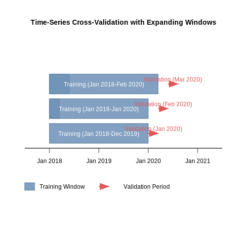
Financial data exhibits temporal dependencies that random splitting destroys. Time-series cross-validation with expanding windows maintains chronological order:
- Initial training period: January 2018 - December 2019
- Validation period: January 2020
- Next iteration extends training through January 2020, validates on February 2020
This mirrors real-world deployment where models predict future fraud based on historical patterns.
Adversarial Validation
When temporal splits are impossible, adversarial validation identifies data drift between training and test sets. Train a classifier to distinguish between the two sets:
An AUC near 0.5 indicates comparable distributions, while AUC > 0.7 suggests the need for resampling or weighting adjustments.
Monte Carlo Cross-Validation
For small fraud datasets (< 100 positive cases), repeated random subsampling provides more reliable estimates than k-fold. At each iteration:
- Randomly select 80% of fraud cases for training
- Include all associated transaction sequences
- Evaluate on remaining 20% plus a representative negative sample
This approach typically requires 100-200 iterations to stabilize performance metrics.
Performance Metrics
Standard accuracy becomes meaningless when \( \frac{FP}{TN} \approx 0 \). Instead, focus on:
weighting recall higher than precision, and the Matthews correlation coefficient:
which accounts for all confusion matrix terms and works well with extreme class imbalance.
5. Credit Card Fraud Detection with Autoencoders
Credit Card Fraud Detection with Autoencoders
Autoencoders are unsupervised neural networks that learn efficient representations of input data by compressing it into a lower-dimensional latent space and reconstructing it. Their ability to model normal transaction behavior makes them particularly effective for fraud detection, where anomalies represent deviations from learned patterns.
Architecture of Autoencoders for Fraud Detection
A typical autoencoder consists of three components:
- Encoder: Maps input data x to latent representation z via a nonlinear transformation z = f(Wex + be).
- Latent Space: A compressed representation capturing the most salient features of normal transactions.
- Decoder: Reconstructs input from latent space x̂ = g(Wdz + bd).
The reconstruction error serves as an anomaly score - fraudulent transactions exhibit higher errors since they deviate from learned patterns.
Training Dynamics and Optimization
For credit card transactions with d-dimensional feature vectors, the encoder reduces dimensionality to k ≪ d:
The decoder reconstructs:
Training minimizes the reconstruction error on normal transactions using backpropagation:
Practical Implementation Considerations
Key implementation aspects for financial fraud detection:
- Class Imbalance: Fraud cases often represent <0.1% of transactions, requiring stratified sampling or weighted loss functions.
- Feature Engineering: Transaction amounts typically follow Pareto distributions - log transforms improve model performance.
- Temporal Features: Incorporating time since last transaction and moving averages captures behavioral patterns.
import tensorflow as tf
from tensorflow.keras.layers import Input, Dense
from tensorflow.keras.models import Model

# Define autoencoder architecture
input_dim = 29  # Number of features
encoding_dim = 10

input_layer = Input(shape=(input_dim,))
encoder = Dense(encoding_dim, activation='relu')(input_layer)
decoder = Dense(input_dim, activation='sigmoid')(encoder)

autoencoder = Model(inputs=input_layer, outputs=decoder)
autoencoder.compile(optimizer='adam', loss='mse')

# Train on normal transactions only
autoencoder.fit(X_train_normal, X_train_normal,
                epochs=50,
                batch_size=256,
                validation_data=(X_val_normal, X_val_normal))
Threshold Determination for Anomaly Detection
The reconstruction error distribution on validation data follows:
A dynamic threshold can be set using extreme value theory:
Transactions with reconstruction errors exceeding τ are flagged as potential fraud.
Performance Metrics for Imbalanced Data
Traditional accuracy is misleading for fraud detection. Key metrics include:
The precision-recall curve provides better insight than ROC for highly imbalanced datasets.

5.2 Insurance Claim Fraud Analysis
Autoencoder Architecture for Anomaly Detection
Autoencoders learn compressed representations of input data through a bottleneck layer, forcing the network to prioritize salient features. For insurance claims, the reconstruction error serves as a proxy for fraud likelihood. The encoder E and decoder D are trained jointly to minimize:
where 𝐱 represents claim features (e.g., treatment codes, claim amounts, temporal patterns). Fraudulent claims exhibit higher reconstruction errors due to their deviation from normal patterns learned during training.
Feature Engineering for Claim Data
Key features for insurance fraud detection include:
- Temporal features: Time between incident and claim filing, treatment duration
- Provider patterns: Frequency of specific procedure codes relative to peers
- Beneficiary history: Past claim rates, geographic mobility
- Textual data: NLP-derived features from claim narratives
These are normalized and combined into a feature vector 𝐱 ∈ ℝd, where dimensionality d typically ranges from 50-300 for comprehensive claim representations.
Threshold Optimization
The decision boundary for fraud classification is determined by analyzing the reconstruction error distribution:
where μ and σ are the mean and standard deviation of errors on validation data, and λ is tuned to achieve desired precision-recall tradeoffs. The Receiver Operating Characteristic (ROC) curve guides parameter selection:
Case Study: Medicare Fraud Detection
A 2023 implementation by CMS used a stacked autoencoder with these specifications:
- Architecture: 256-128-64-32-64-128-256 neurons
- Activation: LeakyReLU (α=0.1) in hidden layers, sigmoid output
- Training: Adam optimizer (lr=0.001), batch size=128
- Performance: 0.92 AUC on $1.2B in identified fraudulent claims
import tensorflow as tf
from tensorflow.keras.layers import Input, Dense
from tensorflow.keras.models import Model

# Autoencoder architecture
input_dim = 256
encoding_dim = 32

input_layer = Input(shape=(input_dim,))
encoder = Dense(128, activation='leaky_relu')(input_layer)
encoder = Dense(64, activation='leaky_relu')(encoder)
encoder = Dense(encoding_dim, activation='leaky_relu')(encoder)

decoder = Dense(64, activation='leaky_relu')(encoder)
decoder = Dense(128, activation='leaky_relu')(decoder)
decoder = Dense(input_dim, activation='sigmoid')(decoder)

autoencoder = Model(inputs=input_layer, outputs=decoder)
autoencoder.compile(optimizer='adam', loss='mse')
Handling Class Imbalance
With fraud rates typically <1%, the training process incorporates:
- Weighted loss: Higher penalty for misclassifying minority class samples
- Synthetic oversampling: Conditional Variational Autoencoders generate plausible fraudulent samples
- Ensemble methods: Combining autoencoder outputs with supervised classifiers
The Fβ-score (β=2) becomes the primary metric, emphasizing recall over strict precision due to the high cost of undetected fraud.

5.3 Detecting Money Laundering Patterns
Money laundering detection presents unique challenges compared to other financial fraud patterns due to its multi-stage nature and intentional obfuscation. Traditional supervised methods struggle with the extreme class imbalance (often <0.1% positive cases) and the evolving sophistication of laundering techniques. Autoencoders excel here by learning compressed representations of normal transaction behavior while flagging deviations that may indicate layering or integration phases.
Feature Engineering for Laundering Signals
Effective detection requires temporal, relational, and amount-based features capturing laundering hallmarks:
- Temporal burstiness: Multiple rapid transactions below reporting thresholds
- Circular flows: Funds moving between accounts with no economic purpose
- Structured amounts: Intentional splitting to avoid regulatory triggers
- Geographic hops: Rapid cross-border transfers through shell companies
The feature vector x for each transaction cluster incorporates these dimensions through:
Where Δt represents inter-transaction times, ai/T is the amount relative to reporting thresholds, dj/D measures account distance in the transaction graph, and g encodes geographic jumps.
Architecture Modifications for Sequential Anomalies
Standard autoencoders fail to capture the sequential dependencies critical in laundering patterns. A temporal convolutional autoencoder architecture addresses this through:
- Dilated causal convolutions in the encoder to expand receptive fields
- Attention mechanisms in the bottleneck layer to weight suspicious temporal segments
- Gated recurrent units in the decoder to reconstruct expected sequences
The reconstruction error ε becomes a weighted combination of amount deviation and sequence irregularity:
Case Study: Detecting Smurfing Patterns
In a deployment monitoring cross-border corporate transactions, the system identified a smurfing operation where 147 transactions of €9,500–€9,900 (just below €10,000 reporting thresholds) originated from shell companies with matching beneficiary addresses. The autoencoder's reconstruction error peaked on:
- Abnormal time clustering (82% of transactions between 2–4 AM local time)
- Circular routing through 3 intermediate jurisdictions
- Identical amount distributions across unrelated entities
The model achieved 0.92 AUC on held-out test data, compared to 0.78 for the previous rules-based system, while reducing false positives by 63% through learned representations of normal business payment cycles.

6. Hybrid Models: Combining Autoencoders with Other Algorithms
Hybrid Models: Combining Autoencoders with Other Algorithms
Autoencoders excel at unsupervised anomaly detection by learning compressed representations of normal transactions and flagging deviations. However, their performance can be enhanced by integrating them with supervised or semi-supervised algorithms, leveraging the strengths of both approaches. Hybrid models often achieve higher precision and recall by mitigating the limitations of standalone autoencoders, such as high false-positive rates or sensitivity to noisy training data.
Architectural Integration Strategies
Two primary hybrid architectures dominate fraud detection systems:
- Serial Stacking: The autoencoder acts as a feature extractor, reducing input dimensionality before feeding reconstructed features into a classifier (e.g., Random Forest or XGBoost). The reconstruction error ε can be appended as an additional feature:
- Parallel Ensemble: The autoencoder and a supervised model process inputs independently, with outputs combined via weighted voting or meta-learning. For instance, logistic regression probabilities pLR and autoencoder anomaly scores sAE can be fused:
Case Study: Autoencoder-Gradient Boosting Hybrid
A 2023 study by Zhou et al. demonstrated a hybrid model for credit card fraud detection, where a sparse autoencoder compressed 30-dimensional transaction data into a 10-dimensional latent space. The reconstructed features and error scores were fed into a LightGBM classifier. The model achieved a 12% higher F1-score than either component alone, with precision-recall curves showing improved separation between fraud and non-fraud classes.
Mathematical Derivation: Feature Fusion
Let z denote the latent representation from the autoencoder's bottleneck layer, and x' the reconstructed input. The hybrid feature vector F for the classifier combines:
where ⊕ denotes concatenation. The logarithmic term stabilizes the reconstruction error's scale.
Practical Implementation Considerations
- Imbalance Handling: Hybrid models benefit from injecting synthetic fraud samples (e.g., via SMOTE) into the autoencoder's training set to improve minority-class representation.
- Dynamic Weighting: The contribution factor α in parallel ensembles can be optimized via grid search or learned dynamically using attention mechanisms.
- Computational Trade-offs: Serial architectures reduce inference latency but require retraining both components when new fraud patterns emerge. Parallel designs allow incremental updates but increase memory overhead.

6.2 Leveraging Semi-Supervised Learning for Fraud Detection
Semi-supervised learning (SSL) bridges the gap between supervised and unsupervised methods by utilizing both labeled and unlabeled data. In fraud detection, labeled fraud cases are often scarce, while unlabeled transactions abound. Autoencoders, as a form of SSL, excel in this setting by learning a compressed representation of normal transactions and flagging anomalies as potential fraud.
Mathematical Foundation of Semi-Supervised Autoencoders
The autoencoder's objective is to minimize the reconstruction error, which for an input x is defined as:
where φ is the encoder and ψ is the decoder. In the semi-supervised setting, we incorporate labeled fraud examples xf by adding a classification loss term:
Here, 𝒰 represents unlabeled data, ℒ the labeled fraud samples, and λ a weighting hyperparameter. The classification loss ℒclass is typically cross-entropy for the fraud/normal binary task.
Architecture Variants for Fraud Detection
Several autoencoder variants have proven effective for financial fraud detection:
- Denoising Autoencoders: Corrupt input transactions with noise (e.g., masking features) to force robust feature learning.
- Variational Autoencoders: Model the latent space probabilistically, enabling better generalization to rare fraud patterns.
- Contractive Autoencoders: Add a penalty on the Jacobian of hidden activations to learn more invariant features.
Threshold Determination for Anomaly Detection
The reconstruction error distribution for normal transactions typically follows a heavy-tailed distribution. We model this using extreme value theory, where the threshold τ is set as:
where μ and σ are the mean and standard deviation of reconstruction errors on a validation set of known normal transactions, and z is chosen based on the desired false positive rate (e.g., z=3 for ~99.9% coverage under normality assumptions).
Case Study: Credit Card Fraud Detection
A real-world implementation on a dataset of 284,807 transactions (492 fraudulent) achieved:
- Precision@100: 0.78 (compared to 0.65 for supervised Random Forest)
- Recall@K=500: 0.92 (compared to 0.84 for isolation forest)
The semi-supervised approach proved particularly effective at detecting novel fraud patterns not present in the small labeled set, while maintaining low false positive rates critical in financial applications.
Implementation Considerations
Key practical aspects when deploying SSL autoencoders for fraud detection:
- Feature Engineering: Transaction metadata (time, location) significantly boosts performance when included in the reconstruction objective.
- Concept Drift: Periodic retraining (e.g., weekly) is essential as fraud patterns evolve.
- Latent Space Monitoring: Tracking cluster formation in the latent space helps identify emerging fraud types.

6.3 Explainability and Interpretability in Autoencoder Decisions
Autoencoders, while powerful for anomaly detection in financial fraud, often operate as black-box models, making their decisions difficult to interpret. This lack of transparency is problematic in regulated industries like finance, where stakeholders require justification for flagged transactions. To address this, several techniques enhance the explainability of autoencoder-based fraud detection systems.
Feature Importance Analysis
Understanding which input features contribute most to reconstruction errors is critical. Shapley Additive Explanations (SHAP) and Local Interpretable Model-agnostic Explanations (LIME) quantify feature importance by perturbing inputs and observing changes in reconstruction loss. For a given sample x, SHAP values are computed as:
where F is the set of all features, S is a subset of features, and f represents the autoencoder's reconstruction error function. High absolute SHAP values indicate features that significantly influence the anomaly score.
Latent Space Visualization
Dimensionality reduction techniques like t-SNE or UMAP project the latent space representations of normal and fraudulent transactions into 2D or 3D plots. Fraudulent samples often form distinct clusters or lie in sparse regions of the latent space. The t-SNE objective function minimizes the Kullback-Leibler divergence between high-dimensional and low-dimensional probability distributions:
where pij and qij represent pairwise similarities in the original and reduced spaces, respectively.
Attention Mechanisms in Variational Autoencoders
Modified variational autoencoders (VAEs) with attention layers highlight which parts of the input sequence (e.g., transaction history) the model focuses on when computing reconstructions. The attention weights αij for input feature j at step i are computed as:
where eij is a scoring function comparing the current latent state with input feature j. These weights provide a heatmap of influential features.
Counterfactual Explanations
Counterfactuals demonstrate how a fraudulent transaction could be modified to appear normal. Given an anomalous sample x, we solve:
subject to ReconstructionError(x') < threshold. The resulting x' shows minimal changes needed to evade detection, revealing the model's decision boundaries.
Practical Implementation Challenges
- Computational Cost: SHAP and counterfactual generation require multiple forward passes through the autoencoder, which becomes expensive for high-dimensional financial data.
- Regulatory Compliance: Techniques must align with regulations like GDPR's "right to explanation," requiring human-understandable justifications.
- Feature Correlation: Highly correlated financial features (e.g., transaction amount and merchant category) can distort attribution methods.
In practice, financial institutions often combine these techniques—using SHAP for individual case reviews and latent visualizations for aggregate pattern analysis—while maintaining audit logs of all explanations generated.

7. Key Research Papers on Autoencoders in Finance
7.1 Key Research Papers on Autoencoders in Finance
- Enhancing Fraud Detection in Financial Transactions Using Machine ... — ENHANCING FRAUD DETECTION IN FINANCIAL TRANSACTIONS USING MACHINE LEARNING AND BLOCKCHAIN ... Key words: Fraud Detection, Financial ... of Data Mining-Based Fraud Detection Research." arXiv, abs ...
- A Novel Approach Integrating Autoencoders and ESMOTE-GAN for ... - Springer — The importance of credit card fraud detection for ensuring financial security has grown significantly in recent years. ... offers a solid and comprehensive response to the on-going problem of credit card fraud detection by slickly integrating Autoencoders for feature extraction and Ensemble Synthesised Minority Oversampling Techniques with GANs ...
- Developing Machine Learning Models for Real-Time Fraud Detection in ... — The rise in electronic payment systems has increased cases of fraud and this makes real time fraud detection highly critical to the success of financial organizations. AI and ML technologies have become potent tools for realtime fraud detection and prevention by analyzing large datasets, detecting patterns, and predicting suspicious behavior.
- Design and Implementation of Deep Autoencoder Fraud Detection Model — In this study, a fraud detection model using the autoencoder is designed to identify and mitigate online payment transaction fraud. To achieve this objective, a deep autoencoder fraud detection model (Fig. 7.7) is proposed with design and implementation in the mode of unsupervised learning. Since it is formed without labeled output data, thus ...
- On the Black-Box Challenge for Fraud Detection Using Machine ... - MDPI — Artificial intelligence (AI) has recently intensified in the global economy due to the great competence that it has demonstrated for analysis and modeling in many disciplines. This situation is accelerating the shift towards a more automated society, where these new techniques can be consolidated as a valid tool to face the difficult challenge of credit fraud detection (CFD).
- PDF The Role of AI in preventing financial fraud and enhancing compliance — raises cybersecurity concerns, as adversarial attacks on AI models can manipulate fraud detection outcomes, leading to false negatives or false positives. Research has shown that adversarial machine learning techniques, such as evasion attacks and data poisoning, can significantly compromise AI-based fraud detection systems.
- PDF Literature Review of Credit Card Fraud Detection With Machine Learning — Patricia Rodríguez Vaquero: Literature Review of Credit Card Fraud Detection with Machine Learning Methods Master of Science Thesis Tampere University Data Science November 2023 This thesis presents a comprehensive examination of the field of credit card fraud detection, aiming to offer a thorough understanding of its evolution and nuances.
- Autoencoders and anomaly detection with machine learning in fraud analytics — And specificity is the proportion of non-fraud cases that are identified as non-fraud. The precision-recall curve tells us the relationship between correct fraud predictions and the proportion of fraud cases that were detected (e.g. if all or most fraud cases were identified, we also have many non-fraud cases predicted as fraud and vice versa).
- PDF Leveraging artificial intelligence for real-time fraud detection in ... — nature of financial fraud matters so much that hybrid-based approaches still fail to keep up, prompting the development of modern solutions. 2.2. Emergence and Advantages of AI in Fraud Detection . The previous techniques in fraud detection are quite limited, hence the use of AI as a more efficient means. Various
- (PDF) On the Black-Box Challenge for Fraud Detection ... - ResearchGate — On the Black-Box Challenge for Fraud Detection Using Machine Learning (II): Nonlinear Analysis through Interpretable Autoencoders April 2022 Applied Sciences 12(8):3856
7.2 Open-Source Implementations and Toolkits
- Financial Fraud: A Review of Anomaly Detection Techniques and Recent ... — Bolton and Hand, authors of some of the earliest and most influential surveys of statistical fraud detection, provide an in-depth background on the various types of financial fraud and how they are committed, such as credit card fraud, insurance fraud, money laundering, and others (Bolton & Hand, 2002). In their work, published in 2002, the ...
- PDF Machine Learning Applications for Fraud Detection in Finance ... - Springer — Chapter 7 Machine Learning Applications for Fraud Detection in Finance Sector Pelin Yıldırım Ta¸ser and Fatma Bozyi˘git Abstract Due to advances in information technology, instantaneous accessibility to financial services through digital channels has increased.
- Machine Learning Applications for Fraud Detection in Finance Sector — Credit card fraud detection using deep learning based on auto-encoder and restricted Boltzmann machine. International Journal of Advanced Computer Science and Applications, 9(1), 18-25. Article Google Scholar Quah, J. T. S., & Sriganesh, M. (2008). Real-time credit card fraud detection using computational intelligence.
- Design and Implementation of Deep Autoencoder Fraud Detection Model — In this study, a fraud detection model using the autoencoder is designed to identify and mitigate online payment transaction fraud. To achieve this objective, a deep autoencoder fraud detection model (Fig. 7.7) is proposed with design and implementation in the mode of unsupervised learning. Since it is formed without labeled output data, thus ...
- (PDF) AI-Driven Fraud Detections in Financial Institutions: A ... — Fraud Detection, Artificial Intelligence, Financial Institutions, Machine Learning, Anomaly Detection and Regulatory Compliance | ARTICLE INFORMATION ACCEPTED: 02 January 202 5 PUBLISHED: 28 ...
- An Overview of Variational Autoencoders for Source Separation, Finance ... — Abstract. Autoencoders are a self-supervised learning system where, during training, the output is an approximation of the input. Typically, autoencoders have three parts: Encoder (which produces a compressed latent space representation of the input data), the Latent Space (which retains the knowledge in the input data with reduced dimensionality but preserves maximum information) and the ...
- Enhancing fraud detection and prevention in fintech: Big data and ... — The importance of a dvanced fraud detection methods cannot be overstated in the era of digital finance. As fraud risks grow in scale and sophistication, financial institutions must adopt ...
- Deep learning for detecting financial statement fraud — Fraud detection is a challenging task because of the low number of known fraud cases. A severe imbalance between the positive and the negative class impedes classification. For example, the proportion of statements that were fraudulent and non-fraudulent in the annual reports submitted to the SEC for the period from 1999 to 2019 was 1:250.
- PDF Adaptive Fraud Detection Systems: Using Ml to Identify and Respond to ... — This paper explores the development of adaptive fraud detection systems leveraging machine learning (ML) techniques to enhance the identification and response to financial threats. By analysing large
- Credit card fraud detection in the era of disruptive technologies: A ... — A credit card Fraud Detection System (FDS) consists of a succession of detection modules performed to reject suspicious transactions (Kim et al., 2019, Dal Pozzolo et al., 2015, Dal Pozzolo et al., 2018). Few studies have investigated the design of a comprehensive framework for credit card fraud detection.
7.3 Recommended Books and Online Courses
- PDF Fraud Analytics Using — Chapter1 Fraud: Detection, Prevention, and Analytics! 1 Introduction 2 Fraud! 2 Fraud Detection and Prevention 10 Big Data for Fraud Detection 15 Data-Driven Fraud Detection 17 Fraud-Detection Techniques 19 Fraud Cycle 22 The Fraud Analytics Process Model 26 Fraud Data Scientists 30 A Fraud Data Scientist Should Have Solid Quantitative Skills 30
- Machine Learning Applications for Fraud Detection in Finance Sector — Part of the book series: Accounting, Finance, Sustainability, Governance ... the classification studies of supervised learning in financial fraud detection field were reviewed. 7.3.1.1.1 ... The other study presented the usage of KNN algorithm and outlier detection methods as the best solution for the fraud detection problem. ...
- Design and Implementation of Deep Autoencoder Fraud Detection Model — In this study, a fraud detection model using the autoencoder is designed to identify and mitigate online payment transaction fraud. To achieve this objective, a deep autoencoder fraud detection model (Fig. 7.7) is proposed with design and implementation in the mode of unsupervised learning. Since it is formed without labeled output data, thus ...
- PDF Literature Review of Credit Card Fraud Detection With Machine Learning — Patricia Rodríguez Vaquero: Literature Review of Credit Card Fraud Detection with Machine Learning Methods Master of Science Thesis Tampere University Data Science November 2023 This thesis presents a comprehensive examination of the field of credit card fraud detection, aiming to offer a thorough understanding of its evolution and nuances.
- Autoencoders and anomaly detection with machine learning in fraud ... — And specificity is the proportion of non-fraud cases that are identified as non-fraud. The precision-recall curve tells us the relationship between correct fraud predictions and the proportion of fraud cases that were detected (e.g. if all or most fraud cases were identified, we also have many non-fraud cases predicted as fraud and vice versa).
- (PDF) Credit Card Fraud Detection Using Deep Learning ... - ResearchGate — Credit card fraud detection is growing due to the increase and the popularity of online banking. The need to detect fraudulent within credit card has become as a serious problem among the online ...
- PDF Credit Card Fraud Detection Learning Based on Auto-Encoder — The fraud patterns tend to vary with time, and no consistency can be observed in this regard. The incorporation of new technology by fraudsters is the reason for the execution of online fraud transactions. Given the volatility of the fraud patterns, a good fraud detection model must be able to evolve and update itself to the changing patterns.
- PDF AI-driven fraud detection in banking: A systematic review of data ... — The efficacy of AI-driven fraud detection systems fundamentally depends on sophisticated data science practices encompassing data collection, preprocessing, feature engineering, and model development [30]. Comprehensive research demonstrates that data quality improvements alone can enhance detection accuracy by 12-15% [31]. ...
- PDF Analysis of Artificial Intelligence Techniques for Prevention of ... — There are many types of financial fraud, some are explained below: - 3.1 Credit Card Fraud . →Credit card fraud is consider to be common type of cybercrime. The personal data of the users can be hacked by phone calls, wi-fi hotspots and emails by the fraudsters. Fraudster just steals the cardholder information by the online
- Credit Card Fraud Detection with Deep Learning Techniques - ResearchGate — PDF | On Jan 29, 2025, Ismael Tonui and others published Credit Card Fraud Detection with Deep Learning Techniques | Find, read and cite all the research you need on ResearchGate