Image Inpainting with Diffusion
1. Problem Definition and Use Cases
1.1 Problem Definition and Use Cases
Image inpainting refers to the task of reconstructing missing or corrupted regions in an image while maintaining coherence with the surrounding context. Mathematically, given an input image I with a masked region M, the goal is to generate a plausible completion I' such that:
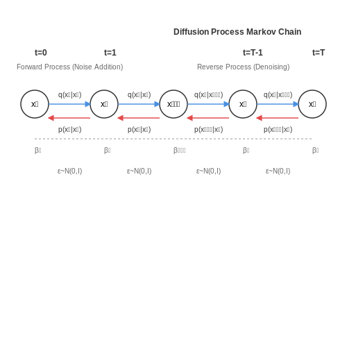
where fθ represents the inpainting model with parameters θ. Diffusion models approach this problem through iterative denoising, where the model learns to gradually reconstruct the masked region by reversing a Markov chain of noise additions.
Technical Challenges
Diffusion-based inpainting must address several key challenges:
- Boundary consistency: The generated content must seamlessly blend with the unmasked regions at the mask boundaries.
- Semantic coherence: The inpainted content should be semantically meaningful and contextually appropriate.
- High-frequency detail preservation: The reconstruction should maintain realistic textures and fine details.
Diffusion Formulation
The forward diffusion process gradually adds Gaussian noise to the image according to a variance schedule βt:
For inpainting, the reverse process is conditioned on the observed pixels outside the mask. At each denoising step t, the model predicts the noise component for the masked region while preserving the known pixels:
Practical Applications
Diffusion-based inpainting has significant real-world applications:
- Photo restoration: Repairing damaged historical photographs or removing artifacts.
- Object removal: Eliminating unwanted elements from images while maintaining background consistency.
- Medical imaging: Completing missing regions in MRI or CT scans for improved diagnosis.
- Creative editing: Generating novel content in specified image regions for artistic applications.
Performance Metrics
Quantitative evaluation typically employs:
where PSNR measures pixel-level accuracy and SSIM evaluates structural similarity. For semantic evaluation, Fréchet Inception Distance (FID) compares feature distributions between generated and real images.

1.2 Traditional Inpainting Methods and Their Limitations
Diffusion-Based Inpainting
Diffusion-based methods formulate inpainting as a partial differential equation (PDE) problem, where pixel values propagate from known regions into missing areas through iterative diffusion. The anisotropic diffusion equation governs this process:
where I represents the image intensity, g(·) is a diffusion coefficient function that preserves edges, and ∇ denotes the spatial gradient. While effective for small gaps, these methods suffer from:
- Excessive blurring across strong edges due to imperfect edge-stopping functions
- Inability to hallucinate semantically plausible structures in large missing regions
- Sensitivity to the initialization of missing regions
Exemplar-Based Techniques
Exemplar-based approaches like Criminisi's algorithm decompose the inpainting task into:
where Ψ represents image patches, and SSD computes sum-of-squared differences. These methods:
- Rely heavily on the availability of similar texture patches in the known regions
- Struggle with structural continuation when geometric priors are weak
- Produce visually inconsistent results when copying patches across dissimilar semantic regions
Variational Methods
Variational formulations minimize an energy functional combining data fidelity and regularization terms:
where φ(·) is a convex regularizer. While theoretically elegant, these approaches:
- Require careful tuning of the regularization parameter λ
- Often produce over-smoothed results due to convexity requirements
- Lack mechanisms for semantic understanding of image content
Fundamental Limitations
All traditional methods share three critical weaknesses when compared to modern diffusion-based approaches:
- Local vs. global understanding: They operate on low-level features without semantic awareness
- Deterministic nature: Cannot generate multiple plausible hypotheses for missing content
- Scale sensitivity: Performance degrades rapidly with increasing hole size relative to image dimensions
The inability to model complex priors over natural images fundamentally limits their application to real-world scenarios where missing regions often require semantically meaningful synthesis rather than simple interpolation or copying.
1.3 Introduction to Diffusion Models
Diffusion models are a class of generative models that learn to synthesize data by gradually denoising a normally distributed variable. The process is inspired by non-equilibrium thermodynamics, where a system evolves from a high-entropy state (noise) to a low-entropy state (structured data) through iterative refinement. Unlike GANs or VAEs, diffusion models operate by defining a fixed forward process that corrupts data with Gaussian noise and then learning a reverse process that systematically removes this noise.
Forward and Reverse Processes
The forward process is a Markov chain that gradually adds Gaussian noise to the data over T timesteps. Given an input image x0, the forward process generates a sequence x1, x2, ..., xT where:
Here, βt is a noise schedule that determines how much noise is added at each step. The reverse process learns to approximate the true posterior q(xt-1 | xt) by training a neural network to predict the noise component:
The model is trained to minimize the variational lower bound (VLB) on the negative log-likelihood, which simplifies to a denoising objective:
where ε is the noise added during the forward process and εθ is the model's noise prediction.
Denoising Diffusion Probabilistic Models (DDPM)
DDPMs formalize the diffusion process by parameterizing the reverse transitions with a neural network. The key insight is that the reverse process can be approximated by a Gaussian distribution if the forward process uses small noise steps. The mean μθ is typically reparameterized to predict the noise εθ directly:
where αt = 1 - βt and ᾱt = ∏s=1t αs.
Score-Based Interpretation
Diffusion models can also be interpreted as score-based generative models, where the score function ∇x log p(x) is approximated by the noise predictor. The score function describes the direction in which the data density increases most rapidly, guiding the denoising process:
This connection links diffusion models to stochastic differential equations (SDEs), where the denoising process is viewed as solving a reverse-time SDE.
Practical Considerations
Training diffusion models requires careful tuning of the noise schedule βt and the architecture of εθ. Common choices include:
- Linear or cosine noise schedules to balance fast convergence and sample quality.
- U-Net architectures with residual connections and attention mechanisms for εθ.
- Classifier-free guidance to trade off diversity and fidelity in conditional generation.
Sampling from diffusion models is iterative and computationally expensive, requiring T forward passes of the network. Recent advances, such as DDIM (Denoising Diffusion Implicit Models), accelerate sampling by using non-Markovian reverse processes without sacrificing quality.

2. Denoising Diffusion Probabilistic Models (DDPM)
Denoising Diffusion Probabilistic Models (DDPM)
Denoising Diffusion Probabilistic Models (DDPM) formulate image generation as an iterative denoising process, reversing a fixed Markov chain that gradually corrupts data with Gaussian noise. The forward process q is defined as:
where βt is a noise schedule increasing from β1 to βT over T timesteps. The forward process admits closed-form sampling at arbitrary timesteps:
where αt = 1 - βt and \(\bar{\alpha}_t = \prod_{s=1}^t \alpha_s\). The reverse process learns to iteratively denoise through a neural network εθ predicting noise from noisy inputs:
Training Objective
DDPM minimizes a reweighted variant of the ELBO, focusing on the noise prediction term:
where \(x_t = \sqrt{\bar{\alpha}_t}x_0 + \sqrt{1-\bar{\alpha}_t}\epsilon\) and \(\epsilon \sim \mathcal{N}(0,\mathbf{I})\). This simplification yields more stable training than the full variational bound.
Sampling Process
Sampling iteratively refines noise over T steps using the learned reverse transitions:
where \(z \sim \mathcal{N}(0,\mathbf{I})\) and \(\sigma_t^2 = \beta_t\). Recent variants employ deterministic samplers (DDIM) for accelerated generation.
Connection to Score-Based Models
DDPMs implicitly learn the score function \(\nabla_{x_t} \log p(x_t)\) through the noise prediction network, as:
This links diffusion models to score-based generative modeling, enabling techniques like annealed Langevin dynamics.
Architectural Considerations
Common architectures use U-Nets with:
- Residual blocks with group normalization
- Attention layers at multiple resolutions
- Sinusoidal position embeddings for timestep conditioning
- Learned variance prediction for \(\Sigma_θ(x_t,t)\)

Training and Inference in Diffusion Models
Forward and Reverse Diffusion Processes
The forward diffusion process gradually adds Gaussian noise to an image x0 over T timesteps according to a predefined schedule. At each step t, the noised sample xt is generated by:
where βt represents the noise schedule. The reverse process learns to gradually denoise the image by estimating pθ(xt-1|xt), typically parameterized as:
Training Objective
The model is trained to minimize the variational lower bound (VLB) on the negative log likelihood. In practice, this reduces to predicting either the noise component or the clean image at each step. The simplified objective for noise prediction is:
where ε is the actual noise added during the forward process and εθ is the neural network's prediction. The network architecture typically uses a U-Net with residual blocks and attention mechanisms.
Sampling and Inference
During inference, sampling starts from pure noise xT ∼ 𝒩(0,I) and iteratively applies the learned reverse process:
where z ∼ 𝒩(0,I), αt = 1-βt, and σt controls the stochasticity. For image inpainting, the known regions are conditioned at each step using:
while the unknown regions are updated by the model predictions.
Practical Considerations
Several techniques improve training stability and sample quality:
- Noise scheduling: Cosine or learned schedules often outperform linear schedules
- Guidance: Classifier-free guidance amplifies conditional signals
- Acceleration: DDIM sampling allows fewer steps while maintaining quality
- Precision: Mixed-precision training is essential for large models
The choice of architecture details like the number of residual blocks, attention heads, and channel multipliers significantly impacts both training efficiency and final performance. Recent variants employ transformer-based architectures or hybrid approaches for improved scaling.

2.3 Adapting Diffusion Models for Inpainting Tasks
Diffusion models excel at generating high-quality images by iteratively denoising random noise, but adapting them for inpainting requires conditioning the generation process on the known regions of the image. The key challenge lies in ensuring the inpainted regions remain consistent with the surrounding context while preserving structural coherence.
Conditional Denoising for Inpainting
Given a corrupted image xmasked with a binary mask m (where 1 indicates known pixels and 0 indicates missing regions), the inpainting task involves sampling from the conditional distribution p(xmissing | xknown). The denoising process is modified to incorporate the known pixels at each timestep t:
where ⊙ denotes element-wise multiplication. This ensures the known pixels remain fixed while the model focuses on denoising only the masked regions. The denoising network εθ is trained to predict noise for the entire image but is evaluated only on the masked regions during sampling.
Gradient-Based Guidance
To enhance semantic consistency, gradient-based guidance can be applied by modifying the predicted noise with the gradient of a perceptual loss:
where λ controls the strength of guidance and ℒperc measures feature-level similarity between the generated and known regions using a pre-trained network like VGG. This encourages the inpainted content to align with the surrounding context.
Blended Diffusion
An alternative approach blends the denoised output with the known pixels at each step using a schedule that gradually increases blending strength:
The blending weights αt follow a cosine schedule, starting near 0 (strong conditioning) and approaching 1 (weak conditioning) as t decreases. This allows early steps to focus on structural alignment while later steps refine details.
Practical Considerations
- Mask shape sensitivity: Irregular masks often yield better results than rectangular ones by providing more diverse boundary conditions.
- Noise schedule adjustment: Slower noise decay (smaller βt) helps maintain coherence for large missing regions.
- Post-processing: Poisson blending or edge-aware filtering can mitigate discontinuities at mask boundaries.

3. Data Preparation and Mask Generation
3.1 Data Preparation and Mask Generation
Effective image inpainting with diffusion models requires carefully curated training data and strategically generated masks. The quality of the inpainted results is directly influenced by the diversity of the dataset and the realism of the masks used during training. This section covers the key considerations for data preparation and mask generation in diffusion-based inpainting systems.
Dataset Requirements
The training dataset should encompass a wide variety of scenes, objects, and textures to ensure the diffusion model learns robust feature representations. For general-purpose inpainting, large-scale datasets like ImageNet, COCO, or Places365 are commonly used. Domain-specific applications may require custom datasets (e.g., medical images for healthcare applications). Key dataset characteristics include:
- High resolution: Minimum 256×256 pixels, preferably higher for detailed inpainting
- Diverse content: Multiple object categories, scenes, and lighting conditions
- Balanced distribution: Avoid overrepresentation of specific classes or features
- Clean annotations: Properly labeled segmentation masks when available
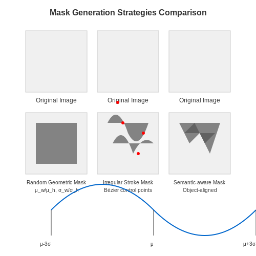
Mask Generation Strategies
The mask generation process determines what portions of the image the model must inpaint during training. Several approaches exist for creating realistic masks:
Random Geometric Masks
Simple but effective masks can be generated using random geometric shapes. The probability density function for generating rectangular masks of width w and height h follows:
where Z is the normalization constant, and μw, μh define the mean mask dimensions (typically 20-40% of image size) with σw, σh controlling size variation.
Irregular Masks
More realistic masks can be generated using random strokes or brush patterns. These better simulate real-world damage or object removal scenarios. The stroke generation process involves:
- Initialize mask with zeros
- Generate random Bézier curves with control points sampled from a normal distribution
- Apply varying stroke widths along each curve
- Combine multiple strokes until desired occlusion percentage is reached
Semantic-Aware Masks
For object removal tasks, masks should align with object boundaries. This requires either:
- Using existing segmentation masks from annotated datasets
- Applying off-the-shelf segmentation models (e.g., Mask R-CNN) to automatically generate object masks
Preprocessing Pipeline
The complete data preparation pipeline involves several transformation steps:
def preprocess_image(image, mask):
    # Normalize pixel values
    image = image / 255.0
    # Apply data augmentation
    if training:
        image, mask = random_augmentation(image, mask)
    # Combine image and mask
    masked_image = image * (1 - mask)
    # Add noise for diffusion process
    noisy_image = add_diffusion_noise(masked_image)
    return {
        'original': image,
        'masked': masked_image,
        'noisy': noisy_image,
        'mask': mask
    }
Validation Considerations
When preparing the validation set, maintain separate mask generators to prevent data leakage. Common validation scenarios include:
- Central masks: Large centered occlusions testing completion ability
- Corner masks: Testing boundary condition handling
- Thin structures: Narrow masks testing edge continuation
- Multiple objects: Masks covering several objects simultaneously
3.2 Model Architecture Choices
The effectiveness of diffusion-based image inpainting hinges on the architectural design of the underlying neural network. Two primary architectures dominate the field: U-Net-based diffusion models and transformer-based diffusion models. Each has distinct advantages in handling spatial dependencies, computational efficiency, and scalability.
U-Net-Based Diffusion Models
U-Nets are the de facto standard for diffusion models due to their ability to capture multi-scale features through skip connections. The architecture consists of an encoder-decoder structure with residual blocks and attention mechanisms. The forward process is modeled as:
where βt is the noise schedule. The U-Net learns to reverse this process by predicting the noise component:
Key modifications for inpainting include:
- Partial Convolutions: Mask-aware convolutions that only process valid pixels, preventing leakage from corrupted regions.
- Gated Attention: Dynamically weights feature importance based on the mask, improving inpainting coherence.
- Multi-Resolution Loss: Applies reconstruction losses at different scales to enhance detail preservation.
Transformer-Based Diffusion Models
Vision transformers (ViTs) have emerged as competitive alternatives, particularly for high-resolution inpainting. The self-attention mechanism allows global context modeling, which is critical for large missing regions. The diffusion process is reformulated in token space:
Architectural innovations include:
- Masked Token Prediction: Only inpaints masked tokens, reducing computational overhead.
- Axial Attention: Decomposes 2D attention into row-wise and column-wise operations for efficiency.
- Adaptive Token Pruning: Dynamically drops less relevant tokens to handle large images.
Hybrid Architectures
Recent work combines U-Nets and transformers, such as using a U-Net for local feature extraction and a transformer for global coherence. The hybrid approach achieves state-of-the-art results on benchmarks like Places2 and CelebA-HQ, with PSNR improvements of 1.5–2 dB over pure architectures.
Computational trade-offs must be considered: U-Nets are more memory-efficient for high resolutions (e.g., 1024×1024), while transformers excel at capturing long-range dependencies but require careful optimization to scale.

3.3 Training Strategies and Hyperparameter Tuning
Noise Scheduling and Diffusion Steps
The noise schedule determines how progressively noise is added and removed during training and inference. A well-designed schedule balances computational efficiency and generation quality. The forward process gradually corrupts an image \(x_0\) with Gaussian noise over \(T\) steps, following:
where \(\beta_t\) is the noise schedule. Common choices include:
- Linear schedule: \(\beta_t = \beta_0 + t(\beta_T - \beta_0)/T\)
- Cosine schedule: \(\beta_t = \cos^{-1}\left(\frac{t}{T} \cdot \frac{\pi}{2}\right)\)
- Sigmoid schedule: \(\beta_t = \sigma\left(\frac{t - T/2}{s}\right)\)
The cosine schedule often outperforms linear scheduling due to smoother transitions between noise levels, reducing abrupt artifacts during denoising.
Loss Function and Training Dynamics
Diffusion models are trained to predict noise \(\epsilon\) at each timestep \(t\). The loss function is typically:
where \(\epsilon_\theta\) is the neural network. Variants include:
- Simple MSE loss: Directly minimizes noise prediction error.
- Weighted loss: Applies timestep-dependent weights \(w(t)\) to focus on critical denoising steps.
- Perceptual loss: Incorporates VGG or LPIPS metrics to enhance structural coherence.
Hyperparameter Optimization
Key hyperparameters and their tuning strategies:
Learning Rate and Batch Size
Diffusion models benefit from large batch sizes (e.g., 256–1024) and adaptive learning rates. The Adam optimizer with warmup is commonly used:
- Initial learning rate: \(1e-4\) to \(5e-4\)
- Warmup steps: 5k–10k iterations
- Batch size: Scales with GPU memory, but larger batches stabilize training.
Architecture Choices
The U-Net backbone requires careful design:
- Depth and width: 4–6 down/up blocks with 128–512 channels.
- Attention layers: Self-attention at lower resolutions (e.g., 16×16) improves global coherence.
- Residual connections: Critical for gradient flow in deep networks.
Practical Considerations
Training diffusion models for inpainting introduces additional constraints:
- Mask augmentation: Randomly vary mask shapes and sizes to improve generalization.
- Gradient clipping: Prevents instability during long training runs.
- Mixed-precision training: FP16/FP32 hybrid reduces memory usage without sacrificing quality.
Case Study: Stable Diffusion Inpainting
Stable Diffusion’s inpainting pipeline uses:
- Noise schedule: Cosine with \(T=1000\) steps.
- Loss: MSE with VGG perceptual loss weighting.
- Batch size: 512 on 8×A100 GPUs.
Empirical results show that fine-tuning the noise schedule and loss weighting reduces artifacts in high-resolution inpainting (≥512×512).
3.4 Evaluation Metrics for Inpainting Quality
Quantitative evaluation of image inpainting results requires carefully designed metrics that capture perceptual quality, structural coherence, and fidelity to the original data. While human judgment remains the gold standard, automated metrics enable scalable benchmarking of diffusion-based inpainting models.
Pixel-Level Metrics
Traditional pixel-wise comparisons measure the discrepancy between inpainted regions I and ground truth G:
where MAXI represents the maximum possible pixel value. While computationally efficient, these metrics often correlate poorly with human perception, particularly for diffusion-based outputs where plausible hallucinations may deviate from ground truth while remaining visually convincing.
Perceptual Metrics
Feature-space metrics better align with human judgment by comparing deep representations:
where φl denotes activations from layer l of a pretrained network (typically VGG or AlexNet), and wl are learned weights. The Learned Perceptual Image Patch Similarity (LPIPS) metric has demonstrated strong correlation with human rankings of inpainting quality.
Structural Similarity
The SSIM index decomposes image similarity into luminance, contrast, and structure components:
where μ and σ represent local means and standard deviations, while C1, C2 stabilize the division. Multi-scale extensions (MS-SSIM) improve performance by evaluating similarity across resolution pyramids.
Fréchet Inception Distance
For evaluating the statistical quality of inpainted regions, FID compares distributions in Inception-v3 feature space:
where (μr, Σr) and (μg, Σg) are the mean and covariance of real and generated features respectively. Lower FID values indicate better alignment with natural image statistics.
Task-Specific Metrics
For semantic inpainting applications, segmentation-based metrics quantify object-level consistency:
- mIoU: Mean Intersection-over-Union between inpainted and ground truth segmentations
- Boundary F-score: Precision-recall measure for contour alignment
- Semantic Consistency: CLIP similarity between text prompts and inpainted regions
Recent work has introduced diffusion-specific metrics like Inception Score for diversity evaluation and Precision/Recall curves for fidelity-coverage tradeoff analysis. The choice of metrics should align with the intended use case—restoration tasks prioritize fidelity metrics, while creative applications may emphasize diversity measures.
4. Conditional Diffusion Models for Guided Inpainting
4.1 Conditional Diffusion Models for Guided Inpainting
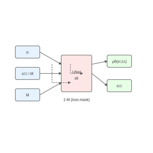
Conditional diffusion models extend standard denoising diffusion probabilistic models (DDPMs) by incorporating auxiliary information to guide the generation process. In image inpainting, this conditioning typically takes the form of a binary mask M indicating missing regions and the observed pixels xobs. The forward process remains identical to unconditional diffusion, but the reverse process learns to sample missing content xmiss conditioned on xobs.
Conditional Reverse Process
The key modification occurs in the reverse transition, where the denoising network εθ now takes both the noisy image xt and the conditioning signal as input. For inpainting, we formulate the conditional reverse process as:
where ⊙ denotes element-wise multiplication. The mean μθ is predicted by a neural network that processes the concatenation of the noisy image and the masked observed pixels.
Training Objective
The training loss extends the standard DDPM objective by focusing only on the missing regions:
This formulation ensures the model only learns to predict noise for the masked regions while preserving the observed content. The conditioning is implemented via concatenation or attention mechanisms in the UNet architecture.
Guidance Strategies
Several approaches exist to strengthen the conditioning:
- Hard Conditioning: Directly replace known pixels at each sampling step using:
$$ x_t^{obs} = \sqrt{\bar{\alpha}_t} x_0^{obs} + \sqrt{1-\bar{\alpha}_t} \epsilon $$
- Soft Conditioning: Use classifier-free guidance by randomly dropping the conditioning signal during training and interpolating between conditional and unconditional predictions during sampling.
- Attention-Based Conditioning: Employ cross-attention layers where the observed pixels serve as keys/values for the missing region queries.
Architectural Modifications
Effective conditional inpainting requires specialized architectures:
- Gated Convolutions: Learn dynamic feature selection based on the mask to prevent leakage between known and unknown regions.
- Partial Convolutions: Normalize activations only by the unmasked pixels in each receptive field.
- Multi-Scale Conditioning: Inject the conditioning signal at multiple UNet resolution levels through adaptive instance normalization (AdaIN) or feature concatenation.
Sampling Considerations
The sampling procedure requires careful handling of noise schedules and conditioning:
where c represents the conditioning information and z ~ 𝒩(0,I). The observed pixels are resampled at each step according to the forward process to maintain consistency.
4.2 Accelerating Diffusion Sampling for Faster Inference
The primary computational bottleneck in diffusion models lies in the iterative sampling process, which typically requires hundreds to thousands of sequential denoising steps to generate high-quality samples. For image inpainting applications where real-time or interactive performance may be desired, this slow inference speed poses significant practical limitations.
Denoising Diffusion Implicit Models (DDIM)
DDIMs reformulate the diffusion process as a non-Markovian chain while maintaining the same training objective as DDPMs. This allows for deterministic sampling along a learned trajectory, enabling high-quality generation in significantly fewer steps. The update rule for DDIM sampling is given by:
where σt controls the stochasticity of the process (set to 0 for deterministic sampling) and zt ∼ N(0,I). By carefully selecting the noise schedule {αt}, DDIM can achieve comparable sample quality in 10-50 steps versus the 1000+ required by standard DDPM.
Stochastic Differential Equation (SDE) Solvers
The continuous-time interpretation of diffusion models as discretizations of an underlying SDE enables the application of advanced numerical integration techniques. The probability flow ODE corresponding to the reverse-time SDE is:
where f(x,t) and g(t) are the drift and diffusion coefficients respectively. High-order Runge-Kutta methods or predictor-corrector schemes can substantially reduce the number of required function evaluations while maintaining sample quality.
Latent Space Diffusion
Operating the diffusion process in a compressed latent space rather than pixel space dramatically reduces computational requirements. The latent representation z = E(x) is obtained via a pretrained autoencoder, with the diffusion model trained to denoise in this lower-dimensional space:
After diffusion sampling in latent space, the final image is decoded via x = D(z0). This approach reduces memory usage and accelerates sampling by 5-10× while maintaining perceptual quality.
Knowledge Distillation
Multi-step diffusion samplers can be distilled into fewer-step student models through:
where fθ(T) represents the teacher's T-step denoising process and fφ(S) the student's S-step approximation (S ≪ T). Progressive distillation can further compress the sampling process into very few steps (as few as 4-8) while preserving sample quality.
Adaptive Step Sizing
Dynamic adjustment of step sizes during sampling based on local curvature estimates can optimize the tradeoff between speed and accuracy. The optimal step size Δt at each point can be estimated via:
This allows for larger steps in flatter regions of the denoising landscape while taking smaller steps near critical points where the score function changes rapidly.

Handling Complex Scenes and High-Resolution Images
Challenges in High-Resolution Inpainting
Diffusion models face significant computational and memory constraints when processing high-resolution images due to the quadratic growth of attention operations in transformer-based architectures. For an image of resolution H × W, the computational complexity of self-attention scales as O(H²W²), making it impractical for resolutions beyond 512×512 without optimization.
where b is batch size, h is attention heads, l is layers, and hw is the number of patches. This necessitates architectural innovations for feasible high-resolution inpainting.
Multi-Scale Diffusion Approaches
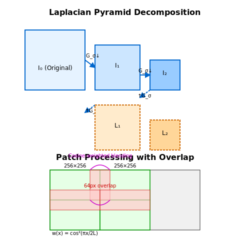
Hierarchical diffusion frameworks address this by decomposing the inpainting task across multiple resolution levels. The Laplacian pyramid decomposition provides a mathematical foundation:
where Gσ is a Gaussian kernel. The diffusion process operates independently at each level, with cross-scale attention mechanisms maintaining global coherence. This reduces memory usage by approximately 60% for 1024×1024 images compared to monolithic approaches.
Patch-Based Processing Strategies
For complex scenes with mixed foreground/background structures, patch-based diffusion with overlap-tile blending proves effective. The algorithm:
- Divides the image into overlapping 256×256 patches
- Processes each patch independently with 64px overlap
- Blends results using a cosine-weighted window function:
where s is the overlap region width. This maintains continuity while allowing parallel processing.
Attention Optimization Techniques
Sparse attention patterns and windowed attention reduce computational overhead. The shifted window approach partitions the image into non-overlapping M×M windows, with successive layers using:
This maintains a receptive field of 2M×2M while keeping complexity linear with image size. For a 1024×1024 image with M=64, this reduces attention operations by 256× compared to global attention.
Memory-Efficient Gradient Calculation
Checkpointing and reversible layers enable training with limited GPU memory. The memory savings come from recomputing activations during backpropagation rather than storing them:
where N is the number of layers. This allows training diffusion models with up to 128 layers on a single GPU for 2K resolution images.
Practical Implementation Considerations
When implementing high-resolution inpainting systems:
- Use mixed-precision training with gradient scaling to maintain stability
- Implement progressive growing of resolution during training
- Employ spectral normalization in all convolutional layers
- Leverage teacher forcing for complex structural inpainting
The trade-off between patch size and global coherence becomes critical above 2048×2048 resolutions, often requiring hybrid approaches that combine patch-based processing with low-resolution global guidance.
5. Key Research Papers on Diffusion Models
5.1 Key Research Papers on Diffusion Models
- Localization of diffusion model-based inpainting through the inter ... — The demand for research into image detection models specialized for images generated by diffusion models is increasing. However, studies on detecting forged images created by diffusion models are relatively scarce [21]. Because diffusion models tend to generate more realistic images in both the pixel and frequency domains compared to ...
- Inst-Inpaint: Instructing to Remove Objects with Diffusion Models — Index Terms—Instruction-based inpainting, diffusion models. 1 INTRODUCTION Image inpainting refers to the task of removing unwanted objects and/or filling in missing regions within an im-age [5], [26], [32]. It is considered highly challenging as the inpainted regions in the resulting images should be in harmony with the rest of the images.
- PDF SmartBrush: Text and Shape Guided Object Inpainting with Diffusion Model — training object inpainting with text-to-image genera-tion to leverage more training data. 2. Related Work Diffusion Models Diffusion models (DMs) [7,24] learn the data distribution by inverting a Markov noising pro-cess, and they have gained wide attention recently due to their stability and superior performance in image synthesis as compared ...
- Diffuse to Choose: Enriching Image Conditioned Inpainting in Latent ... — Image Editing, particularly inpainting, has been extensively explored in diffusion models. Initially, there were text-based image editing models [ 25 , 2 , 9 , 13 , 14 ] . However, it is evident that text alone cannot capture the fine-grained details necessary for accurately describing a product, necessitating the use of image conditioning.
- Image inpainting using diffusion models to restore eaves tile patterns ... — This paper proposes a coarse-to-fine image inpainting method based on the denoising diffusion probabilistic model (DDPM), specifically optimized for wadang pattern restoration. The method starts with an initial inpainting phase, followed by a fusion module that combines the semantic information of the input image with intermediate outputs to ...
- Ship-Go: SAR Ship Images Inpainting via instance-to-image Generative ... — Download: Download high-res image (258KB) Download: Download full-size image Fig. 1. Ship-Go is an instance-to-image diffusion model. It can edit images conditioned on the visual instance and environment prompt, and place objects in the background of specified environmental types, which enables Ship-Go to extend instance datasets to instance-level recognition datasets (e.g., object detection).
- CrackDiffusion: crack inpainting with denoising diffusion models and ... — The main inspiration of traditional image inpainting methods is to use the texture features to fill the missing regions of an image. Early works attempt to utilize background patches close to the missing regions, gradually padding from the boundary to the center of missing regions [].However, these methods assume the lost information is the copy of background, and thus it is hard to reproduce ...
- PDF Towards Coherent Image Inpainting Using Denoising Diffusion Implicit Models — Image inpainting refers to the task of generat-ing a complete, natural image based on a par-tially revealed reference image. Recently, many research interests have been focused on address-ing this problem using fixed diffusion models. These approaches typically directly replace the revealed region of the intermediate or final gen-
- Exploring Image Transformations with Diffusion Models: A Survey of ... — The main contribution of the paper is the development of a new training procedure for diffusion models that enables the use of text prompts to guide image synthesis. The proposed method, called GLIDE, achieves SOTA results in image synthesis and editing tasks, such as super-resolution, inpainting, and style transfer.
- Fill in the (a diffusion-based image inpainting pipeline) - arXiv.org — Stochastic inpainting techniques, such as flow-based and MLM-based methods, utilize generative models and sequence prediction to reconstruct image structures and textures. Additionally, many stochastic techniques take the approach of starting with a noisy image and iteratively denoise it until reaching a sensible output, a strategy commonly ...
5.2 Open-Source Implementations and Toolkits
- Feature pyramid network for diffusion-based image inpainting detection — First, we implement our experiments on the detection of the diffusion-based inpainting without post-processing. 40,000 images randomly selected from the COCO dataset [37] and center-cropped to 384 × 512 are used to generate diffusion-based inpainting samples with the method provided by G'MIC [38], an open-source framework for image manipulation.
- Fill in the (a diffusion-based image inpainting pipeline) - arXiv.org — Fill in the (a diffusion-based image inpainting pipeline) Eyoel Gebre * ... p = 0.5 𝑝 0.5 p=0.5 italic_p = 0.5 (2) Figure 5: Images generated with ... In this study, we aimed to improve image inpainting techniques by enhancing control over what exactly gets generated. In particular, we identified that current approaches did not allow a model ...
- BrushNet: A Plug-and-Play Image Inpainting Model with Decomposed Dual ... — Initial attempts at utilizing diffusion models for text-guided inpainting [23, 2, 1, 20, 50, 6, 47], such as Blended Latent Diffusion, modifies the standard denoising strategy by sampling the masked regions from a pre-trained diffusion model and the unmasked areas from the given image, which is commonly used as the default inpainting choice in ...
- Image inpainting using diffusion models to restore eaves tile patterns ... — Image inpainting is an image processing technique used to restore or fill in missing and damaged parts of an image [12]. This technique can be applied to restore old photographs and repair corrupted images. Image inpainting methods can be divided into two categories: texture synthesis-based methods and deep learning-based methods.
- Advanced Video Inpainting Using Optical Flow-Guided Efficient Diffusion — In recent years, diffusion models [22, 9] have revolutionized the field of content generation, showcasing exceptional abilities in creating highly realistic outputs [21, 2].The development of text-to-video (T2V) [7, 10] and image-to-video (I2V) [30, 3] diffusion generative models, has paved the way for innovations in text-guided video inpainting. . Models like AVID [36] and CoCoCo [38], have ...
- Top 23 inpainting Open-Source Projects - LibHunt — Which are the best open-source inpainting projects? This list will help you: InvokeAI, IOPaint, lama, mmagic, manga-image-translator, stablediffusion-infinity, and BallonsTranslator. ... Unlock the magic 🪄: Generative-AI (AIGC), easy-to-use APIs, awsome model zoo, diffusion models, for text-to-image generation, image/video restoration ...
- GitHub - Acly/krita-ai-diffusion: Streamlined interface for generating ... — Inpainting: Use selections for generative fill, expand, to add or remove objects; Live Painting: Let AI interpret your canvas in real time for immediate feedback.Watch Video; Upscaling: Upscale and enrich images to 4k, 8k and beyond without running out of memory.; Diffusion Models: Supports Stable Diffusion 1.5, and XL.Partial support for Flux and SD3. ...
- Ship-Go: SAR Ship Images Inpainting via instance-to-image Generative ... — Download: Download high-res image (258KB) Download: Download full-size image Fig. 1. Ship-Go is an instance-to-image diffusion model. It can edit images conditioned on the visual instance and environment prompt, and place objects in the background of specified environmental types, which enables Ship-Go to extend instance datasets to instance-level recognition datasets (e.g., object detection).
- Connecting image inpainting with denoising in the homogeneous diffusion ... — While local methods for image denoising and inpainting may use similar concepts, their connections have hardly been investigated so far. The goal of this work is to establish links between the two by focusing on the most foundational scenario on both sides - the homogeneous diffusion setting. To this end, we study a denoising by inpainting (DbI) framework. It averages multiple inpainting ...
- IOPaint - PyPI — Features. Completely free and open-source, fully self-hosted, support CPU & GPU & Apple Silicon. Windows 1-Click Installer. OptiClean: macOS & iOS App for object erase. Supports various AI models to perform erase, inpainting or outpainting task.. Erase models: These models can be used to remove unwanted object, defect, watermarks, people from image.; Diffusion models: These models can be used ...
5.3 Recommended Tutorials and Courses
- Diffusion-based image inpainting with internal learning — Diffusion models are now the undisputed state-of-the-art for image generation and image restoration. However, they require large amounts of computational power for training and inference. In this paper, we propose lightweight diffusion models for image inpainting that can be trained on a single image, or a few images. We show that our approach competes with large state-of-the-art models in ...
- PDF Image Guided Inpainting with Parameter Efficient Learning - CVF Open Access — synthesize images they want in various ways with natural language descriptions. In this paper, We tried here to gain control over image creation and to semantically compose images where the user wants. 3. Preliminaries 3.1. Diffusion model The diffusion model generates an image with its inverse process from the diffusion process, which ...
- Inst-Inpaint: Instructing to Remove Objects with Diffusion Models — Index Terms—Instruction-based inpainting, diffusion models. 1 INTRODUCTION Image inpainting refers to the task of removing unwanted objects and/or filling in missing regions within an im-age [5], [26], [32]. It is considered highly challenging as the inpainted regions in the resulting images should be in harmony with the rest of the images.
- Stable Diffusion Inpainting: A Practical Guide for Beginners - Daisie Blog — Stable diffusion inpainting is a versatile technique with numerous real-world applications. In this section, we'll explore how it can be used in image restoration, 3D modeling and animation, and digital art and design. Image Restoration. One of the most common uses for stable diffusion inpainting is in the restoration of damaged or deteriorated ...
- Master AI Image Editing with Stable Diffusion's Inpainting ... - Toolify — A: To further enhance your image editing skills with Stable Diffusion, you can explore online resources, forums, and tutorials specifically focused on this topic. Websites like GitHub and Stack Overflow can provide valuable insights and guidance from the Stable Diffusion community.
- Image inpainting with diffusion models - LinkedIn — Explore how diffusion models can be used to fill in missing parts of images and discover the practical applications of image inpainting. In this video, learn about the concept and process of image ...
- GitHub - Sanster/IOPaint: Image inpainting tool powered by SOTA AI ... — Erase models: These models can be used to remove unwanted object, defect, watermarks, people from image. Diffusion models: These models can be used to replace objects or perform outpainting. Some popular used models include: runwayml/stable-diffusion-inpainting; diffusers/stable-diffusion-xl-1.-inpainting-.1; andregn/Realistic_Vision_V3. ...
- Stable Diffusion: Img2Img-Inpainting-Sketching - Building Simplexity Lab — DESCRIPTION This tutorial introduces users to the features of img2img, Sketching, and Inpainting in Automatic1111, offering enhanced control over image transformation and editing. By explaining the functionalities of sketching, inpainting, and key settings like CFG scale and denoising strength, users can learn how to effectively use these tools to manipulate images according to their preferences.
- AI Art for Beginners - Stable Diffusion Crash Course — AI Art for Beginners - Stable Diffusion Crash Course Syllabus Overview. play_circle On-Demand Video Lecture. timer Watch Duration: 10:31. article Full Lecture Notes. ... Image Inpainting & Outpainting With Stable Diffusion. play_circle On-Demand Video Lecture. timer Watch Duration: 18:48.
- Google Colab — Outpainting with Stable Diffusion on an infinite canvas. The project is powered by the Stable Diffusion inpainting model and has been transformed into a web app using PyScript and Gradio. Results may vary, and users can improve outcomes by adjusting prompts and selections [ ]