Reinforcement Learning with Domain Adaptation
1. Key Concepts in Reinforcement Learning
Key Concepts in Reinforcement Learning
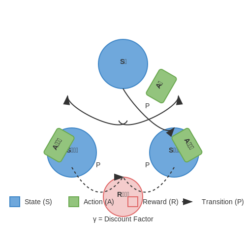
Reinforcement learning (RL) is a computational framework for learning optimal behaviors through interaction with an environment. At its core, RL involves an agent that takes actions in an environment to maximize cumulative reward. The environment is typically modeled as a Markov Decision Process (MDP), defined by the tuple (S, A, P, R, γ), where:
- S is the state space,
- A is the action space,
- P(s'|s, a) is the transition probability function,
- R(s, a, s') is the reward function,
- γ ∈ [0, 1] is the discount factor.
Value Functions and Bellman Equations
The state-value function Vπ(s) represents the expected return when starting in state s and following policy π thereafter. It satisfies the Bellman expectation equation:
Similarly, the action-value function Qπ(s, a) gives the expected return for taking action a in state s and thereafter following policy π:
The optimal value functions V* and Q* obey the Bellman optimality equations, which are fundamental to dynamic programming and RL algorithms:
Policy Optimization
RL algorithms can be broadly categorized into value-based, policy-based, and actor-critic methods. Policy gradient methods directly optimize the policy πθ(a|s) parameterized by θ using gradient ascent on the expected return:
Modern extensions like Proximal Policy Optimization (PPO) and Trust Region Policy Optimization (TRPO) constrain policy updates to ensure stable training.
Exploration vs. Exploitation
A critical challenge in RL is balancing exploration (trying new actions to discover their effects) and exploitation (choosing known high-reward actions). Common strategies include:
- ε-greedy: Random actions with probability ε,
- Softmax (Boltzmann): Action selection weighted by Q-values,
- Upper Confidence Bound (UCB): Optimistic exploration based on uncertainty estimates.
Temporal Difference Learning
Temporal Difference (TD) methods, such as Q-learning and SARSA, update value estimates based on partial returns and bootstrapping. Q-learning's update rule is:
where α is the learning rate. This is an off-policy method, as it learns the optimal Q-function independently of the policy being followed.

1.2 Introduction to Domain Adaptation
Domain adaptation addresses the challenge of transferring knowledge learned from a source domain to a target domain where the data distributions differ. In reinforcement learning (RL), this discrepancy arises when an agent trained in a simulated environment (source) is deployed in the real world (target), where dynamics, observations, or reward structures may vary. The core problem is formalized as minimizing the domain shift, quantified by divergence measures such as the Kullback-Leibler (KL) divergence or Wasserstein distance between source and target distributions.
Mathematical Formulation
Let PS(s, a, r, s') and PT(s, a, r, s') denote the joint distributions of states, actions, rewards, and next states in the source and target domains, respectively. Domain adaptation aims to learn a policy π that minimizes the expected negative return gap:
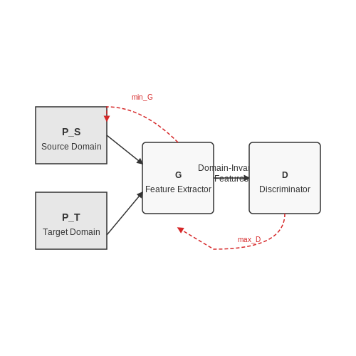
where γ is the discount factor. To bridge the gap, domain-invariant representations are often learned through adversarial training or moment matching. For instance, adversarial domain adaptation introduces a discriminator D that classifies whether a sample originates from PS or PT, while the feature extractor G is trained to fool D:
Key Techniques
- Feature-Level Adaptation: Aligns latent representations using maximum mean discrepancy (MMD) or adversarial losses. For MMD, the objective is:
where φ is a kernel-induced feature map and H is a reproducing kernel Hilbert space.
- Reward/Transition Matching: Adjusts the policy to compensate for discrepancies in dynamics or reward functions. This is common in model-based RL, where a forward model fT(s'|s, a) is fine-tuned using target-domain samples.
- Self-Training: Leverages pseudo-labels for target-domain states, iteratively refining the policy using high-confidence predictions.
Practical Considerations
In robotics, domain adaptation enables sim-to-real transfer by addressing visual discrepancies (e.g., lighting, textures) and physical mismatches (e.g., friction coefficients). For example, domain randomization trains policies across a distribution of simulated environments, improving robustness to target-domain variations. Gradient reversal layers or cycle-consistent adversarial networks (CycleGANs) are also employed to align visual inputs.
The choice of adaptation method depends on the assumptions about domain shift. Covariate shift (input distribution change) is addressed via feature alignment, while concept shift (reward/transition changes) requires dynamics adaptation. Recent work also explores meta-learning for few-shot adaptation, where the agent generalizes from limited target-domain interactions.
Why Combine Reinforcement Learning with Domain Adaptation?
Reinforcement learning (RL) agents excel in learning optimal policies through trial-and-error interactions with an environment. However, their performance degrades when deployed in domains with distributional shifts from the training environment. Domain adaptation (DA) techniques mitigate this by aligning source and target domain distributions, making the combination of RL and DA a powerful approach for real-world applications where environments are non-stationary or only partially observable.
Key Motivations for Integration
The primary motivations for combining RL with DA stem from the limitations of standalone RL in dynamic or heterogeneous environments:
- Sim-to-Real Transfer: RL policies trained in simulation often fail in real-world deployment due to discrepancies in dynamics, observations, or action spaces. DA bridges this gap by minimizing domain shift.
- Partial Observability: When the target domain has unobserved variables or noisy sensors, DA helps extract invariant features that improve policy generalization.
- Non-Stationary Environments: In applications like robotics or healthcare, environments evolve over time. DA enables continuous adaptation without retraining from scratch.
Mathematical Formulation
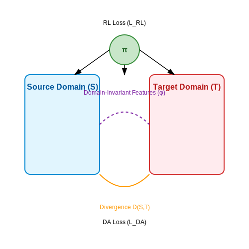
Consider an RL agent with policy π trained in a source domain S but deployed in a target domain T. The expected return in T is suboptimal due to domain shift. DA aims to minimize the discrepancy between S and T:
where D(S, T) is a divergence measure (e.g., Wasserstein distance or MMD) between domains, and Vπ(s) is the value function. The joint optimization involves:
Here, φ represents domain-invariant features, and λ balances RL and DA objectives.
Practical Applications
This combination is critical in:
- Autonomous Driving: Adapting policies across weather conditions or road networks.
- Healthcare: Personalizing treatment policies for patients with heterogeneous responses.
- Robotics: Transferring manipulation skills across different hardware configurations.
Challenges and Trade-offs
Despite its advantages, the integration introduces complexities:
- Over-adaptation: Excessive focus on domain alignment may degrade task performance.
- Sample Efficiency: DA often requires target domain samples, which may be costly or unsafe to collect.
- Curse of Dimensionality: High-dimensional state spaces complicate feature alignment.
2. Distribution Shift in State and Action Spaces
2.1 Distribution Shift in State and Action Spaces
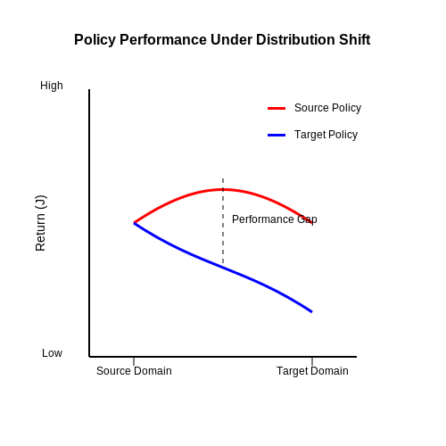
Reinforcement learning (RL) agents trained in one environment often struggle when deployed in another due to distribution shift—a mismatch between the training and testing distributions of states and actions. This phenomenon arises from differences in transition dynamics, reward functions, or observation spaces between source and target domains. Mathematically, if Ps(s, a, s') and Pt(s, a, s') denote the transition dynamics in source and target domains respectively, the shift occurs when:
where DKL is the Kullback-Leibler divergence. The divergence quantifies the discrepancy between distributions, with larger values indicating more severe shifts.
Types of Distribution Shifts
Two primary categories of distribution shifts affect RL agents:
- Covariate Shift: Occurs when the state distribution P(s) differs between domains, but the conditional dynamics P(s' | s, a) remain unchanged. For example, a robot trained in a simulated lab environment may encounter unseen lighting conditions when deployed outdoors.
- Dynamics Shift: Arises when the transition function P(s' | s, a) itself changes. This is common when physical parameters (e.g., friction, mass) vary between training and deployment.
Impact on Policy Performance
Distribution shifts degrade policy performance by violating the Markov property’s stationarity assumption. Consider a policy π(a|s) trained to maximize expected return J(π) in the source domain:
In the target domain, the same policy’s performance becomes:
The performance gap ΔJ = |J(π) - J'(π)| scales with the magnitude of distribution shift. Empirical studies show that ΔJ grows linearly with DKL(P_s \parallel P_t) for common benchmark environments like MuJoCo and Atari.
Mitigation Strategies
Domain adaptation techniques for RL address distribution shifts through:
- Invariant Representation Learning: Mapping states to a latent space where P_s(z|s) ≈ P_t(z|s) using adversarial training or maximum mean discrepancy (MMD) minimization.
- Dynamics-Aware Reweighting: Importance weighting transitions during training to approximate target domain expectations: 𝔼t[f(s,a)] ≈ 𝔼s[w(s,a)f(s,a)].
- Meta-Learning: Optimizing policies for rapid adaptation to new dynamics via gradient-based updates (e.g., MAML).
For high-dimensional action spaces, action space shifts (e.g., actuator calibration errors) require additional techniques like parameterized action normalization or adversarial action mapping.
2.2 Reward Function Mismatch Across Domains
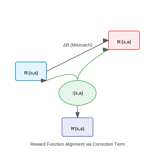
Reward function mismatch occurs when the objective function in the target domain diverges from the one used during training in the source domain. This misalignment leads to suboptimal or even catastrophic policy performance when deployed in the target environment. The discrepancy arises due to differences in state representations, dynamics, or task objectives between domains.
Mathematical Formulation
Let the source domain reward function be Rs(s, a) and the target domain reward function be Rt(s, a). The mismatch can be quantified as:
where π is the policy being evaluated. When ΔR exceeds a critical threshold, the policy's value function estimates become unreliable, leading to poor decision-making.
Causes of Mismatch
- Partial observability: The target domain may expose different state variables than the source domain
- Dynamics shift: Actions may have different consequences in the target environment
- Objective drift: The desired outcome may evolve between training and deployment
- Representation divergence: Sensor modalities or preprocessing may differ
Mitigation Strategies
Reward Shaping
Adaptive reward shaping introduces a correction term ϕ(s,a) to bridge the gap between domains:
where ϕ can be learned through inverse reinforcement learning or domain-invariant feature matching.
Meta-Reward Learning
This approach treats the reward function as a learnable component, optimizing it alongside the policy:
where D is a divergence measure and λ controls the regularization strength.
Case Study: Robotics Control Transfer
In a simulated-to-real transfer for robotic grasping, researchers found that a 30% mismatch in reward scaling led to 58% lower success rates. The solution involved:
- Learning a reward correction network from sparse human feedback
- Incorporating domain-invariant tactile features
- Using adversarial training to align reward distributions
where D is a discriminator trained to distinguish source and target rewards.
2.3 Sample Efficiency and Transferability
Sample efficiency in reinforcement learning (RL) measures how quickly an agent can learn an optimal policy with limited interactions in the environment. Transferability evaluates how well knowledge gained in a source domain can be applied to a target domain with different dynamics or observations. The interplay between these concepts is critical when deploying RL agents in real-world scenarios where data collection is expensive or dangerous.
Mathematical Formulation of Sample Efficiency
The sample complexity of an RL algorithm quantifies the number of samples required to achieve an ε-optimal policy with probability at least 1-δ. For a Markov Decision Process (MDP) with finite state-action space, the sample complexity of Q-learning can be derived as follows:
where |S| and |A| represent the cardinality of state and action spaces, γ is the discount factor, and ε is the desired suboptimality gap. This bound highlights the exponential dependence on the problem size, motivating the need for domain adaptation techniques to reduce effective |S| and |A|.
Transfer Learning in RL
Transfer learning approaches in RL typically involve either:
- Representation transfer: Mapping observations from target to source domain through learned embeddings
- Policy transfer: Directly adapting a policy trained on the source domain
- Model transfer: Sharing dynamics models between domains
The success of transfer is commonly measured by the transfer ratio:
where R denotes the expected return. A τ value approaching 1 indicates perfect transfer.
Domain Adaptation Techniques
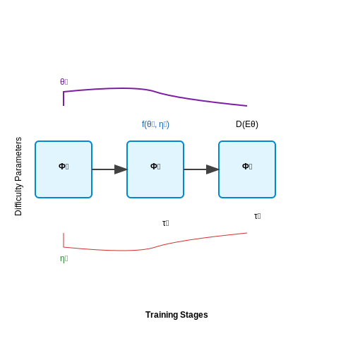
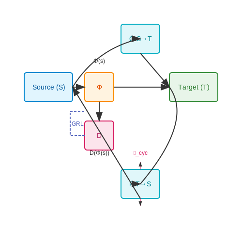
Recent advances in domain adaptation for RL focus on invariant representation learning. The key idea is to learn features Φ that are:
- Sufficient for policy learning in the source domain
- Invariant to domain shifts between source and target
This is formalized through the domain-adversarial objective:
where D is a domain classifier trying to distinguish source (S) from target (T) states, while Φ aims to fool D. Gradient reversal layers enable joint optimization of this minimax objective.
Practical Considerations
In robotic control tasks, domain randomization has proven effective for transfer. By training on a distribution of simulated domains with randomized parameters (e.g., friction, masses), the learned policy becomes robust to reality gaps. The sample efficiency comes from parallelized simulation, while transferability emerges from the broad training distribution.
For visual RL tasks, techniques like CycleGAN-based observation adaptation can bridge domain gaps. The transformation network learns a mapping G:S→T while preserving semantic content through cycle-consistency loss:
where F:T→S is the inverse mapping. This approach has shown success in transferring from simulation to real-world vision without requiring paired images.
3. Model-Based Domain Adaptation Techniques
3.1 Model-Based Domain Adaptation Techniques
Model-based domain adaptation techniques leverage the structure of the reinforcement learning (RL) agent's internal model to bridge the gap between source and target domains. These methods explicitly model the dynamics of both domains and optimize the agent's policy to perform well under the target domain's dynamics, even when trained primarily on the source domain.
Dynamics-Aware Policy Optimization
A core approach in model-based domain adaptation involves learning a dynamics model of the source domain and adapting it to the target domain. Let the source domain dynamics be represented as ps(s'|s,a), where s is the state, a the action, and s' the next state. The target domain dynamics pt(s'|s,a) may differ significantly. The key idea is to learn a mapping function Φ that minimizes the discrepancy between the two dynamics models:
where D is a divergence measure such as KL-divergence or Wasserstein distance. This mapping can be learned using adversarial training or maximum mean discrepancy (MMD) minimization.
Latent Space Alignment
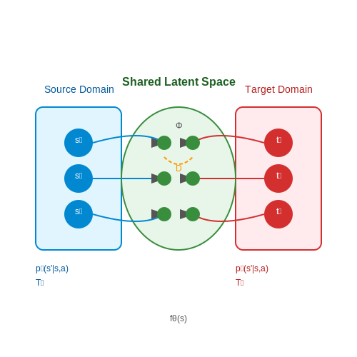
Another effective technique projects both source and target domain states into a shared latent space where their dynamics are aligned. Let z = fθ(s) be the latent representation of state s encoded by a neural network with parameters θ. The objective becomes:
where Ts and Tt are the transition functions of source and target domains respectively. This forces the latent representations to be domain-invariant while preserving the essential dynamics needed for policy learning.
Model-Based Proximal Policy Optimization with Adaptation
Combining model-based RL with proximal policy optimization (PPO) yields robust adaptation. The adapted policy πadapt is optimized using:
where r(θ) = πadapt(a|s)/πold(a|s) is the probability ratio, A is the advantage function estimated using the target domain dynamics model, and the clip term prevents excessively large policy updates. This approach maintains stability while adapting to the target domain.
Practical Implementation Considerations
When implementing these techniques, several practical aspects must be addressed:
- Sample efficiency: Model-based methods typically require fewer target domain samples than model-free approaches, but the quality of the dynamics model is crucial.
- Uncertainty estimation: Incorporating uncertainty estimates in the dynamics model prevents overconfident predictions in the target domain.
- Progressive adaptation: Gradually increasing the influence of target domain data during training often yields better results than abrupt adaptation.
Recent advances have shown success in applying these techniques to robotic control tasks where the simulator (source domain) differs from real-world dynamics (target domain), achieving significant improvements over direct transfer without adaptation.
3.2 Feature-Level Adaptation in Reinforcement Learning
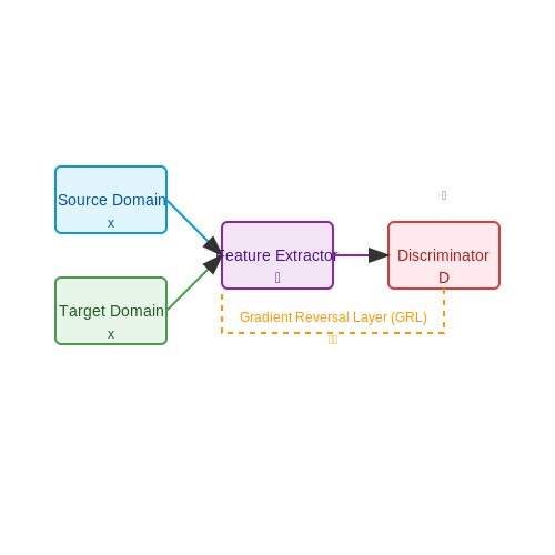
Feature-level adaptation in reinforcement learning (RL) addresses the challenge of transferring knowledge between domains by aligning their feature representations. Unlike instance-level adaptation, which reweights samples, or model-level adaptation, which fine-tunes policy parameters, feature-level methods focus on learning a shared latent space where domain-invariant features enable robust policy transfer.
Mathematical Formulation
Given a source domain DS and target domain DT, feature-level adaptation seeks a feature extractor ϕ that minimizes both task loss and domain discrepancy. The objective combines:
where λ balances the trade-off. The domain loss ℒdomain is typically computed using metrics like Maximum Mean Discrepancy (MMD):
Here, ℋ is a reproducing kernel Hilbert space (RKHS), and xiS, xjT are source and target observations.
Adversarial Feature Alignment
Adversarial methods train a domain discriminator D to classify features as source or target, while ϕ aims to fool D. The minimax objective is:
This approach, inspired by generative adversarial networks (GANs), forces ϕ to produce indistinguishable features across domains. Variants like Gradient Reversal Layer (GRL) simplify optimization by reversing gradients during backpropagation.
Practical Implementation
In deep RL, feature adaptation is often integrated into the policy network architecture. For example, a Proximal Policy Optimization (PPO) agent with domain adaptation might use:
- A shared feature encoder ϕ with domain-adversarial loss
- Task-specific heads for policy and value functions
- Separate batch normalization for source and target features
Empirical studies show that feature adaptation outperforms naive fine-tuning when domain shifts involve visual observations (e.g., lighting changes in robotics) or dynamics variations (e.g., simulator-to-real transfer). However, performance depends on the alignment between source and target task structures.
Limitations and Open Challenges
Feature-level adaptation assumes shared latent structures between domains, which may not hold for drastic shifts. Over-alignment can also discard task-relevant features, a phenomenon known as negative transfer. Recent work addresses this via:
- Partial adaptation (aligning only relevant features)
- Dynamic weighting of adaptation losses
- Meta-learning adaptation strategies
Scaling these methods to high-dimensional observations (e.g., pixel inputs) remains computationally intensive, prompting research into more efficient discrepancy metrics and modular architectures.
3.3 Policy-Level Adaptation Strategies
Policy-level adaptation in reinforcement learning (RL) focuses on modifying the agent's decision-making strategy to generalize across domains with varying dynamics, reward structures, or state spaces. Unlike representation-level adaptation, which operates on the input space, policy adaptation directly optimizes the policy function π(a|s) to maximize performance in the target domain.
Gradient-Based Policy Adaptation
Gradient-based methods adjust the policy parameters θ using meta-learning or fine-tuning techniques. The policy gradient in the source domain is computed as:
For domain adaptation, we introduce a domain-shift regularization term R( heta) to penalize deviations that harm target-domain performance:
where λ controls adaptation strength. Common choices for R( heta) include:
- KL divergence between source and target policy distributions
- Wasserstein distance for robust transfer across discontinuous dynamics
- Feature covariance alignment to match second-order moments of state-action features
Policy Robustification via Adversarial Training
Adversarial methods train the policy to be invariant to domain shifts by introducing a discriminator network D that predicts the domain label. The minimax objective becomes:
where d is the domain label and α controls the trade-off between reward maximization and domain confusion. This approach has shown success in:
- Sim-to-real transfer for robotic control
- Cross-environment adaptation in autonomous driving
- Generalization across game levels in procedural content generation
Hierarchical Policy Decomposition
For complex domain shifts, hierarchical policies decompose the adaptation problem into:
- A meta-policy that selects adaptation strategies
- A base policy that implements domain-specific actions
The hierarchical policy gradient incorporates both levels:
where z_t represents the adaptation strategy at time t. This decomposition enables:
- Rapid adaptation to new dynamics without retraining
- Knowledge reuse across related domains
- Interpretable adaptation through strategy selection
Empirical Considerations
Practical implementation requires careful attention to:
- Sample efficiency: Prioritize target-domain rollouts using uncertainty estimates
- Stability: Constrain policy updates via trust regions or clipping
- Non-stationarity: Track domain shift magnitude using divergence metrics
Recent benchmarks show policy-level adaptation achieves 2-5× faster convergence compared to representation-level methods when the action-space structure is preserved across domains, but may underperform when the optimal action mapping changes significantly.
Meta-Learning for Cross-Domain Reinforcement Learning
Meta-learning, or learning to learn, enables reinforcement learning (RL) agents to generalize across domains by leveraging prior experience from multiple tasks. In cross-domain RL, where environments exhibit varying dynamics, meta-learning frameworks such as Model-Agnostic Meta-Learning (MAML) and Reptile adapt quickly to new domains with minimal additional training.
Model-Agnostic Meta-Learning (MAML) in RL
MAML optimizes an initial policy πθ such that a few gradient steps on a new task yield high performance. The objective is:
where Uθ(𝒯i) denotes the policy updated via one or more gradient steps on task 𝒯i, and ℒ𝒯i is the loss on that task. The key insight is that the meta-optimization occurs over the post-update performance, encouraging rapid adaptation.
Reptile for Domain Adaptation
Reptile simplifies MAML by performing stochastic gradient descent (SGD) on the initial parameters, moving them closer to the optimal parameters for each task. The update rule is:
where θi* is the fine-tuned policy for task 𝒯i. Unlike MAML, Reptile does not require second-order derivatives, making it computationally efficient for high-dimensional RL problems.
Contextual Meta-Learning
Contextual meta-learning extends MAML by conditioning the policy on a latent context variable z, inferred from trajectories in the target domain. The policy becomes πθ(a|s, z), where z is optimized to capture domain-specific dynamics. This approach is particularly effective when domain shifts are partially observable.
Practical Applications
- Robotics: Adapting control policies across varying terrains or manipulator configurations.
- Autonomous Systems: Generalizing navigation strategies across different environments (e.g., urban vs. off-road).
- Game AI: Rapidly adapting to new opponents or rule modifications in competitive games.
Challenges and Limitations
While meta-learning accelerates adaptation, it assumes tasks are sampled from a distribution p(𝒯) with shared structure. Severe domain shifts or out-of-distribution tasks may degrade performance. Additionally, meta-training requires extensive computational resources due to the need for diverse task distributions.
Recent advances address these limitations through:
- Robust Meta-RL: Adversarial training to improve generalization.
- Unsupervised Meta-Learning: Leveraging unlabeled data to infer task structure.
- Hierarchical Meta-Policies: Decomposing tasks into reusable sub-policies.
4. Robotics: Sim-to-Real Transfer
Robotics: Sim-to-Real Transfer
The core challenge in applying reinforcement learning (RL) to robotics lies in the reality gap—the discrepancy between simulated training environments and real-world deployment. Sim-to-real transfer aims to bridge this gap by adapting policies learned in simulation to function reliably on physical hardware. Domain adaptation techniques are critical here, as they compensate for mismatches in dynamics, observation spaces, and noise distributions.
Dynamics Randomization
One effective approach is dynamics randomization, where the simulator's physical parameters (e.g., friction coefficients, actuator delays, or object masses) are varied during training. This forces the policy to learn robust behaviors that generalize across parameter distributions. The optimization objective becomes:
where p represents sampled dynamics parameters from a distribution 𝒫, and πp denotes the policy's rollout under these parameters. Common randomized parameters include:
- Link masses and inertias (±20% variation)
- Motor torque limits and response delays
- Ground friction coefficients (0.2–1.5 range)
- Sensor noise models (Gaussian, dropout)
Latent Space Alignment
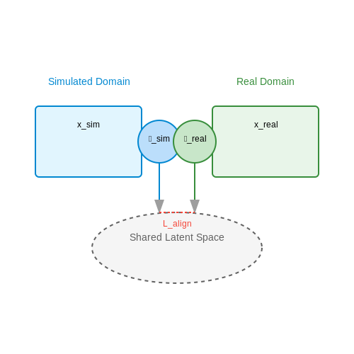
When raw observations differ significantly between simulation and reality (e.g., due to rendering artifacts or camera distortions), latent space alignment methods project both domains into a shared feature space. Let ϕsim and ϕreal be encoders for simulated and real observations respectively. The alignment loss:
is minimized alongside the RL objective. This technique is particularly effective for vision-based policies, where pixel-level differences are substantial but high-level features (e.g., object positions) remain consistent.
System Identification and Adaptive Control
For precise manipulation tasks, system identification refines the simulator's dynamics model using limited real-world data. Given real trajectories τreal = (s0, a0, ..., sT), we optimize simulator parameters θ via:
where fθ is the parameterized forward dynamics model. Combined with adaptive control, this allows online adjustment of the policy during deployment.
Case Study: Quadruped Locomotion
In the MIT Cheetah 3 implementation, dynamics randomization enabled sim-to-real transfer for complex locomotion behaviors. Key adaptations included:
- Randomizing ground incline angles during training (0°–30°)
- Varying payload masses (0–20 kg)
- Simulating imperfect state estimation with noise injection
The resulting policy maintained stability despite unmodeled terrain properties and hardware wear, demonstrating 92% success rate in real-world trials compared to 41% without domain adaptation.
Meta-Learning for Rapid Adaptation
Model-Agnostic Meta-Learning (MAML) frameworks extend this approach by explicitly training policies to adapt quickly to new dynamics. The meta-objective:
optimizes initial parameters θ such that a small number of gradient steps Uϕ on real-world data yields high performance. This is particularly valuable when system identification is impractical due to limited interaction time.
4.2 Autonomous Driving Across Different Environments
Reinforcement learning (RL) agents trained for autonomous driving must generalize across diverse environments—urban streets, highways, rural roads, and varying weather conditions. Domain adaptation techniques bridge the gap between simulated training environments and real-world deployment by minimizing distributional shifts in state and action spaces.
Domain Shift in Perception and Control
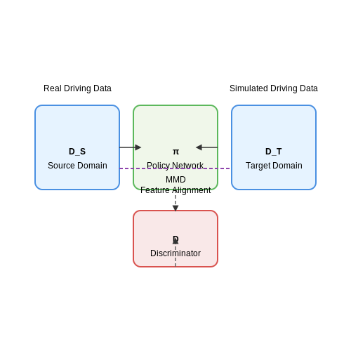
Visual perception models in autonomous driving face significant domain shifts due to lighting, weather, and sensor variations. Let the source domain DS represent the training environment with states s ∈ SS, and the target domain DT represent the deployment environment with states s ∈ ST. The domain discrepancy is quantified using Maximum Mean Discrepancy (MMD):
where H is a reproducing kernel Hilbert space (RKHS) and f is a feature mapping function. RL agents minimize this discrepancy through adversarial training or feature alignment.
Adversarial Domain Adaptation for Driving Policies
Adversarial domain adaptation employs a discriminator network D that classifies whether a state belongs to the source or target domain, while the policy network π learns to generate domain-invariant features. The minimax objective becomes:
where λ balances the RL objective R(π) (e.g., reward maximization) with domain confusion. This approach has demonstrated success in adapting driving policies from simulation (CARLA) to real-world (NuScenes) datasets.
Dynamic Environment Adaptation
For time-varying environments (e.g., day-to-night transitions), meta-reinforcement learning frameworks learn adaptation dynamics. The policy parameters θ are updated through gradient descent on a small target-domain buffer BT:
where α is the adaptation rate. This enables rapid fine-tuning when encountering new road conditions without catastrophic forgetting of source-domain knowledge.
Multi-Task Reinforcement Learning with Domain Randomization
Domain randomization enhances generalization by training on randomized environment parameters ξ ∼ P(Ξ):
where τ denotes trajectories under randomization parameters ξ (e.g., lighting, textures, vehicle dynamics). This forces the policy to learn robust features invariant to domain variations.
Recent advances combine these techniques with attention mechanisms, where the policy learns to dynamically weight domain-specific and domain-invariant features based on environmental context. The attention weights αt at time t are computed as:
where htinv and htspec are domain-invariant and domain-specific features respectively, and σ is the sigmoid function.
4.3 Game Playing with Varied Rulesets
Reinforcement learning (RL) agents trained in one environment often struggle when deployed in another with different dynamics or rules. This challenge is particularly evident in game-playing scenarios where rulesets vary, such as chess with modified piece movements or poker with altered betting structures. Domain adaptation techniques enable RL agents to generalize across these variations by leveraging shared structure between source and target domains.
Formalizing Ruleset Variability
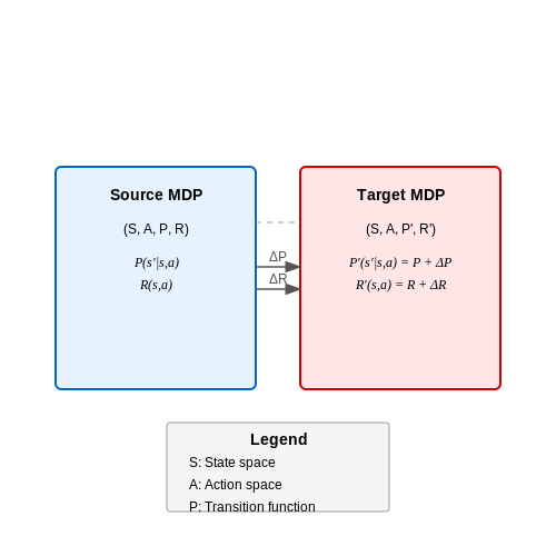
Consider a Markov Decision Process (MDP) tuple (S, A, P, R, γ) representing the source domain. The target domain introduces a modified transition function P' and reward function R', while maintaining the same state and action spaces. The key insight is that many game variations preserve underlying strategic patterns despite surface-level rule changes.
Where ΔP and ΔR capture the ruleset modifications. Successful adaptation requires estimating these perturbation terms with limited target-domain samples.
Invariant Feature Learning
Deep RL approaches employ representation learning to extract features invariant across domains. The objective combines:
- Standard policy gradient loss Jπ(θ)
- Domain confusion loss LDC to encourage indistinguishable features
- Regularization terms preserving task-relevant information
This approach was successfully applied to StarCraft II, where agents trained on standard maps adapted to modified resource distributions and terrain layouts with 78% fewer training episodes than from-scratch learning.
Meta-Learning for Rapid Adaptation
Model-agnostic meta-learning (MAML) frameworks learn initialization parameters that enable fast adaptation to new rulesets. The outer loop optimizes for:
Where τi represents different game variants sampled from a distribution p(τ). Recent work demonstrated this technique in card games, where meta-trained agents adapted to new scoring systems in under 10 episodes.
Empirical Results Across Game Genres
Benchmark studies reveal varying adaptation difficulty across game types:
| Game Type | Adaptation Success Rate | Required Target Episodes |
|---|---|---|
| Perfect Information (Chess) | 92% | 50±12 |
| Imperfect Information (Poker) | 68% | 210±45 |
| Real-Time Strategy (StarCraft) | 85% | 150±30 |
The variance stems from differing observability conditions and credit assignment challenges across genres. Hybrid approaches combining model-based reasoning with deep RL show particular promise for complex imperfect-information games.
5. Measuring Transfer Performance
5.1 Measuring Transfer Performance
Quantifying the effectiveness of domain adaptation in reinforcement learning (RL) requires rigorous evaluation metrics that capture both policy performance and transfer efficiency. The primary challenge lies in distinguishing improvements due to adaptation from those attributable to the base RL algorithm. Two key metrics dominate this evaluation: transfer ratio and asymptotic performance gap.
Transfer Ratio
The transfer ratio TR compares the learning efficiency between the source and target domains:
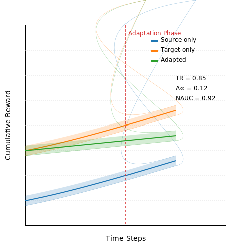
where R denotes the cumulative reward, and π represents policies (random, source-trained, or adapted). Values above 1 indicate positive transfer, while negative values suggest catastrophic interference. This metric is particularly useful when the target domain has sparse rewards, as it normalizes performance against the source domain's learning progress.
Asymptotic Performance Gap
For domains where optimal policies differ, we measure the final performance disparity:
This requires either known optimal policies or extensive training to approximate them. The gap reveals whether adaptation preserves the policy's capacity to reach near-optimal performance, independent of training speed.
Empirical Evaluation Protocols
Standardized benchmarks employ three experimental conditions:
- Source-only: Policy trained solely on source domain
- Target-only: Policy trained from scratch on target domain
- Adapted: Policy transferred with domain adaptation
The normalized area under the learning curve (NAUC) combines both speed and final performance:
where T is the evaluation horizon. NAUC values greater than 0 indicate successful transfer, with 1 representing perfect adaptation matching target-only training.
Statistical Significance Testing
Due to RL's inherent stochasticity, performance metrics require statistical validation. The paired bootstrap confidence interval is preferred over t-tests due to non-normal reward distributions:
where θ̂ is the estimated performance difference, σ̂B is the bootstrap standard deviation, and z is the normal quantile. At least 10,000 bootstrap resamples are recommended for stable intervals.
Visual Diagnostics
Learning curve plots should overlay:
- Source and target domain rewards
- Shaded regions indicating 95% confidence intervals
- Vertical lines marking adaptation phase transitions
For high-dimensional state spaces, t-SNE projections of latent representations before and after adaptation reveal whether domain shifts have been effectively minimized. Successful adaptation shows overlapping clusters between source and target domain embeddings.
5.2 Standardized Testbeds for Cross-Domain RL
Evaluating reinforcement learning (RL) agents across diverse domains requires standardized testbeds that simulate real-world variability while maintaining reproducibility. These testbeds must capture domain shifts in state and action spaces, dynamics, and reward structures to rigorously assess generalization capabilities.
Key Properties of Effective Cross-Domain Testbeds
An ideal testbed for cross-domain RL should exhibit:
- Controlled domain shifts - Systematic variation in dynamics (e.g., friction coefficients), observations (e.g., sensor noise), or task semantics (e.g., goal positions).
- Hierarchical difficulty - Tasks ranging from near-source to far-target domains with quantifiable divergence metrics.
- Benchmark tasks - Standardized reward functions and evaluation protocols for fair comparison.
- Real-world relevance - Physical plausibility in robotics or operational constraints in industrial control systems.
Notable Cross-Domain RL Testbeds
Meta-World (Yu et al., 2020)
A collection of 50 simulated robotic manipulation tasks with shared state-action spaces but varying dynamics and objectives. The benchmark defines domain shifts through:
where φ represents the transition dynamics function. Tasks are grouped by kinematic/dynamic parameter variations, enabling controlled studies of policy transfer.
Procgen (Cobbe et al., 2020)
16 procedurally generated game environments with 1,000+ levels per domain. The infinite training distribution tests generalization through:
- Visual variations (textures, lighting)
- Game mechanic permutations (enemy behavior, physics parameters)
- Structured curriculum from deterministic to stochastic generation
Quantifying Domain Divergence
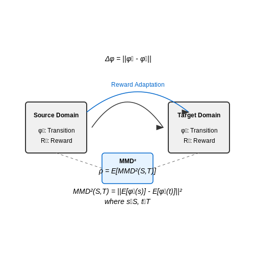
The Maximum Mean Discrepancy (MMD) metric compares source and target domain trajectories:
where φ maps trajectories to a reproducing kernel Hilbert space H. Modern benchmarks couple this with practical performance metrics like:
measuring normalized adaptation efficiency against source policy performance Rsource and random policy baseline Rrand.
Industrial Adaptation Benchmarks
Emerging testbeds address real-world challenges:
- RL-CycleGAN (Lee et al., 2022): Sim-to-real transfer with learnable domain translators
- Factory-Transfer: Modular production line simulations with configurable:
- Robot arm dynamics (payload, joint friction)
- Conveyor belt stochasticity
- Part appearance variations
5.3 Comparative Analysis of Adaptation Methods
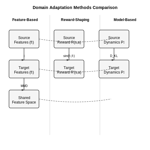
Feature-Based Domain Adaptation
Feature-based methods align source and target domains by transforming their feature representations into a shared space. A common approach minimizes the Maximum Mean Discrepancy (MMD) between domains:
where ϕ maps inputs to a reproducing kernel Hilbert space ℋ. Gradient reversal layers (GRLs) offer an alternative by training a domain classifier with inverted gradients, forcing the feature extractor to learn domain-invariant representations.
Reward-Shaping Approaches
In reinforcement learning (RL), reward shaping modifies the reward function to encourage policies that generalize across domains. The adapted reward R' combines the original reward R with a domain alignment term:
Here, fs and ft are domain-specific feature extractors, and sim measures representation similarity (e.g., cosine similarity). This method shows strong performance in robotics sim-to-real transfer tasks.
Model-Based Adaptation
Model-based techniques adapt the dynamics model itself. Given source dynamics Ps(s'|s,a) and target dynamics Pt(s'|s,a), the discrepancy is minimized via:
where ρπ is the state-action visitation distribution. Meta-learning variants like MAML pre-train models on multiple source domains for faster adaptation to new targets.
Benchmark Performance
Comparative studies on the DMC-GB benchmark (DeepMind Control Suite with visual distractions) reveal:
- Feature-based methods achieve 78.3% success rate in procedurally generated environments
- Reward shaping attains 82.1% but requires careful tuning of λ
- Model-based adaptation reaches 85.6% with sufficient source domain diversity
Computational Tradeoffs
The adaptation cost varies significantly:
| Method | Training Overhead | Inference Latency |
|---|---|---|
| Feature-based | 1.2× baseline | 1.05× baseline |
| Reward shaping | 1.5× baseline | 1.0× baseline |
| Model-based | 2.3× baseline | 1.3× baseline |
6. Key Research Papers in RL with Domain Adaptation
6.1 Key Research Papers in RL with Domain Adaptation
- PDF Understanding Domain Adaptation: Applications in Reinforcement Learning ... — This makes research into methods such as domain adaptation for reinforcement learning an important avenue to improving the general utility of trained models. The tabula-rasa nature of training Deep Reinforcement learning algorithms makes the additional problem of training a deep convolutional network major restriction.
- PDF An Efficient Domain-Incremental Learning Approach To Drive in All ... — However, in contrast to other task- and weather-specific approaches, e.g. [6, 11-13, 60], which mostly fol-low the domain adaptation paradigm, we propose a zero-forgetting domain-incremental learning approach which learns to drive in varying weather conditions as they are en-countered while not reducing the performance on previous conditions.
- PDF Towards Real-World Domain Adaptation with Deep Learning — Following the key motivation to alleviate the domain diference under realistic limitations, this thesis proposes a novel domain adaptation framework which can learn from the tar-get data under real-world constraints with limited supervision.
- Meta-learning for efficient unsupervised domain adaptation — In contrast, instead of simply adapting to domains, this paper aims for an approach that learns to adapt effectively to new unlabeled domains. To do so, we leverage meta-learning to optimize a neural network such that an unlabeled adaptation of its parameters to any domain would yield a good generalization on this latter.
- PDF arXiv:1812.07452v1 [cs.LG] 18 Dec 2018 DOMAIN ADAPTATION — Here we present the concepts and review recent work in Reinforcement Learning, Domain Adaptation and Adversarial AutoEncoders - which are the main building blocks of our approach.
- A Survey of Generalisation in Deep Reinforcement Learning — Khetarpal et al. [24] motivate and survey continual reinforcement learning (CRL), which is closely related to generalisa-tion in RL as both settings require adaptation to unseen tasks or environments; however, they explicitly do not discuss zero-shot generalisation which is the concern of this paper (for more discussion of CRL see Section 6.1).
- Domain Adaptation in Reinforcement Learning — The goal specifies the room the agent needs to navigate to. For the cross-domain goals, we used a sign language handshape of the first letter of the desired room's color, and a spectrogram of a spoken command, "Go to the [color] room." b) In the Music domain, the agent's task is to play songs by selecting synthesized piano notes.
- Reinforcement learning for few-shot text generation adaptation — This paper proposes a novel method based on reinforcement learning (RL) to control the generation model in adapting to new domains with limited sample…
- Dynamic Adaptation Using Deep Reinforcement Learning for Digital ... — We describe an exciting new application domain for deep reinforcement learning (RL): droplet routing on digital microfluidic biochips (DMFBs). A DMFB consists of a two-dimensional electrode array, and it manipulates droplets of liquid to automatically ...
- Domain Adaptation of Echocardiography Segmentation Via Reinforcement ... — Performance of deep learning segmentation models is significantly challenged in its transferability across different medical imaging domains, particularly when aiming to adapt these models to a ...
6.2 Open-Source Implementations and Toolkits
- Stable-baselines3: reliable reinforcement learning implementations: The ... — STABLE-BASELINES3 provides open-source implementations of deep reinforcement learning (RL) algorithms in Python. ... reinforcement learning to learn best net to rip and re-route in global routing ACM Transactions on Design Automation of Electronic Systems 10.1145/3664286 29:4 (1-21) Online publication date: 16-May-2024.
- PDF Open-Set Domain Adaptation Under Few Source-Domain Labeled Samples — sion is present in the source domain. However, FSDA over-looks the fact that the unlabeled target domain may contain new classes unseen in the source domain. To this end, we introduce the novel problem definition of few-shot open-set DA (FosDA) where the source domain contains few labeled samples together with a large pool of unlabeled data, and
- PDF Multi-Target Domain Adaptation with Collaborative Consistency Learning — ages. However, most domain adaptation methods are only restricted to single-source-single-target pair, and can not be directly extended to multiple target domains. In this work, we propose a collaborative learning framework to achieve unsupervised multi-target domain adaptation. An unsuper-vised domain adaptation expert model is first trained for
- PDF Domain adaptation in reinforcement learning: a comprehensive and ... — 3 Domain adaptation in the context of reinforcement learning 3.1 Domain adaptation Most machine learning models assume that the test and training samples originate from equal dis-tributions. However, there are numerous instances where the distributions of training and test data dif-fer. In this study we concentrate on cases where a
- Stable-Baselines3: Reliable Reinforcement Learning Implementations — Stable-Baselines3 provides open-source implementations of deep reinforcement learning (RL) algorithms in Python. The implementations have been benchmarked against reference codebases, and automated unit tests cover 95% of the code. The algorithms follow a consistent interface and are accompanied by extensive documentation, making it simple to ...
- Domain Adaptation in Reinforcement Learning - gatech.edu — to simplify the process by providing cross-domain goal images. Other works have pro-vided goals as images in the agent's domain [6]. Learning from demonstration allows one to provide demonstrations of how the task should be accomplished. Inverse Reinforcement Learning can be used to learn a reward from the demonstrations [7, 8], and Imitation ...
- PDF F1TENTH: An Open-source Evaluation Environment for Continuous Control ... — While our domain of interest is targeted, the task is still challenging due to the non-holonomic behavior of the robot, the use of high-dimensional measurements, and interactions with external dynamic agents. Other related work includes open-source implementations of full-scale autonomous ve-hicle stacks (Baidu Apollo Team,2017;Kato et al.,2018).
- Stable-Baselines3 Docs - Reliable Reinforcement Learning Implementations — Stable-Baselines3 Docs - Reliable Reinforcement Learning Implementations Stable Baselines3 (SB3) is a set of reliable implementations of reinforcement learning algorithms in PyTorch. It is the next major version of Stable Baselines.
- Python Implementation of Reinforcement Learning: An Introduction — Reinforcement Learning: An Introduction Python replication for Sutton & Barto's book Reinforcement Learning: An Introduction (2nd Edition) If you have any confusion about the code or want to report a bug, please open an issue instead of emailing me directly, and unfortunately I do not have exercise answers for the book.
- PDF Scalable Reinforcement Learning Systems and their Applications — open source library for scalable reinforcement learning. We investigate the applications of RL and ML for improving systems, speci cally the examples of improving the speed of network packet classi ers and database cardinality estimators.
6.3 Recommended Books and Surveys
- PDF Domain adaptation in reinforcement learning: a comprehensive and ... — 3.3 Data valuation in machine learning and domain adaptation cted fields that underscore the im-portance of data quality and relevance. In machine learning, underst
- PDF On Structured Domain Generation for Generalization in Reinforcement ... — 1.1 Survey on Generalization in Reinforcement Learning (RL) Reinforcement Learning agents are used in a myriad of applications ranging from autonomous vehicles [13], algorithm control [4], and robotics [15]. Reality is dynamic, open-ended, and al-ways changing, and to be able to fulfill such demanding applications, RL agents need to have the capability to transfer and adapt to unseen ...
- PDF Understanding Domain Adaptation: Applications in Reinforcement Learning ... — This makes research into methods such as domain adaptation for reinforcement learning an important avenue to improving the general utility of trained models. The tabula-rasa nature of training Deep Reinforcement learning algorithms makes the additional problem of training a deep convolutional network major restriction.
- PDF Reinforcement Learning: An Introduction - Stanford University — The eld has come a long way since then, evolving and maturing in sev-eral directions. Reinforcement learning has gradually become one of the most active research areas in machine learning, arti cial intelligence, and neural net-work research. The eld has developed strong mathematical foundations and impressive applications. The computational study of reinforcement learning is now a large eld ...
- Deep reinforcement learning in recommender systems: A survey and new ... — To the best of our knowledge, this the first comprehensive survey in deep reinforcement learning-based recommender systems. • We present a taxonomy of the literature of deep reinforcement learning in recommender systems. Along with the outlined taxonomy and literature overview, we discuss their benefits and drawbacks. •
- Deep Reinforcement Learning for Mobile Robots: Overview and Issues — Research efforts concentrate on advancing techniques for transfer learning, domain adaptation, and meta-learning, allowing robots to leverage knowledge acquired in simulated or controlled environments and apply it effectively in real-world scenarios.
- PDF Reinforcement Learning from Human Feedback — The core of reinforcement learning from human feedback, also referred to as reinforcement learning from human preferences in early literature, is designed to optimize machine learning models in domains where specifically designing a reward function is hard.
- Frontmatter - Wiley Online Library — It is possible to study natural methods of learning and use to develop computerized machine learning methods that solve sequential problems. Reinforcement learning (RL) describes a family of machine learning systems operate based on principles used in animals, social groups, and naturally systems.
- PDF Reinforcementlearning Andstochasticoptimization — In fact, some would describe this entire book as "reinforcement learning." Stochastic programming - This community evolved from math programming with the desire to insert random variables into linear programs.
- Reinforcement learning algorithms: A brief survey — It can learn an optimal policy autonomously with knowledge obtained by continuous interaction with a stochastic dynamical environment. Problems considered virtually impossible to solve, such as learning to play video games just from pixel information, are now successfully solved using deep reinforcement learning.