Stage-wise Difficulty Scaling in RL Environments
1. Definition and Core Principles
Stage-wise Difficulty Scaling in RL Environments: Definition and Core Principles
Stage-wise difficulty scaling in reinforcement learning (RL) refers to the systematic adjustment of environmental complexity, reward sparsity, or action space constraints as a function of an agent's learning progress. Unlike static environments, where the challenge level remains fixed, stage-wise scaling dynamically modulates difficulty to optimize the trade-off between exploration and exploitation.
Formal Definition
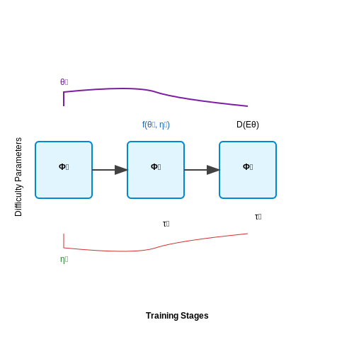
Given an RL environment E with state space S, action space A, and transition dynamics P(s'|s,a), stage-wise difficulty scaling introduces a time-varying parameter vector θt that modifies environment properties:
where θt evolves according to a progression function f that depends on the agent's performance metric ηt:
Core Principles
1. Curriculum Learning Alignment
Stage-wise scaling implements an implicit curriculum by decomposing the learning process into phases {Φ1, ..., Φn}, where each phase introduces progressively harder variations of the task. The transition between phases follows either:
- Threshold-based triggering: Advance when ηt ≥ τk for phase-specific threshold τk
- Continuous adaptation: Smooth interpolation of parameters via θt+1 = θt + α∇θηt
2. Difficulty Metrics
The environmental difficulty can be quantified through multiple axes:
where 𝒟S measures state space complexity (e.g., entropy of P(s'|s,a)), 𝒟A captures action space constraints (e.g., dimensionality reduction factor), and 𝒟R represents reward shaping intensity.
3. Performance-Dependent Scaling
The progression function f typically incorporates:
- Moving average of returns: ηt = (1-β)ηt-1 + βGt
- Success rate: Binary indicators over a sliding window
- Policy entropy: H(π(a|s)) as a measure of exploration
Implementation Variants
Practical implementations differ in how they modify θt:
| Method | Parameter Adjustment | Example Application |
|---|---|---|
| State Space Augmentation | Gradual introduction of distractors or noise | Obstacle density in navigation tasks |
| Action Space Restriction | Progressive removal of action masking | Robotic manipulation with initially constrained joints |
| Reward Shaping Decay | Annealing of dense reward signals | Phased removal of intermediate rewards in sparse-reward games |
Theoretical Foundations
The effectiveness of stage-wise scaling derives from two key theoretical insights:
- Gradient Signal Amplification: Early stages provide higher signal-to-noise ratio for policy gradients by reducing variance in ∇θJ(π).
- Manifold Alignment: Progressive difficulty allows the policy network to develop hierarchical representations that align with the natural curriculum of the task.
This is formalized through the gradient covariance matrix Σt of the policy parameters:
where stage-wise scaling ensures the dominant eigenvalues of Σt grow monotonically with t, preventing premature convergence to suboptimal policies.
Stage-wise Difficulty Scaling in RL Environments: Importance in Reinforcement Learning
Fundamental Role in Training Efficiency
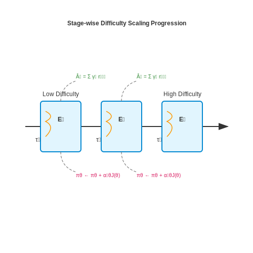
Stage-wise difficulty scaling addresses the exploration-exploitation trade-off by dynamically adjusting environmental complexity. In sparse-reward settings, traditional RL agents often fail due to insufficient exploration. By incrementally increasing difficulty—such as gradually introducing obstacles in navigation tasks—agents learn foundational skills before tackling harder variants. This mirrors curriculum learning, where the agent's policy \(\pi_\theta\) is optimized over a sequence of environments \(\{E_1, E_2, ..., E_n\}\) with progressively stricter dynamics:
Here, \(\hat{A}_t\) denotes the advantage function, and \(\tau\) is a trajectory sampled from the current stage \(E_i\). The gradient updates become more stable as the agent masters simpler tasks first.
Mitigating Catastrophic Forgetting
In continual learning scenarios, abrupt environmental shifts can degrade previously learned policies. Stage-wise scaling introduces intermediate reward shaping and parameterized difficulty (e.g., varying physics parameters in MuJoCo). For instance, a bipedal walker might train first on flat terrain (\(E_1\)) before advancing to uneven slopes (\(E_2\)):
This phased approach reduces catastrophic interference by constraining the policy update space at each stage.
Applications in Real-World Systems
- Robotics: Industrial manipulators learn assembly tasks by progressing from coarse to fine motor control.
- Autonomous Driving: Agents train in low-traffic simulations before advancing to dense urban scenarios.
- Game AI: NPCs adapt to player skill levels by scaling opponent AI difficulty dynamically.
Theoretical Underpinnings
The convergence properties of stage-wise scaling can be analyzed through Markov Decision Process (MDP) hierarchies. Let \(M_i = (S_i, A_i, P_i, R_i)\) represent the MDP for stage \(i\). The optimal policy \(\pi^*\) satisfies:
where \(\gamma\) is the discount factor and \(V^{\pi}\) is the value function. This decomposition ensures that early-stage learning biases later-stage exploration.
Empirical Validation
Recent benchmarks like Procgen and Meta-World demonstrate 2–4× faster convergence with staged training. For example, in Procgen's maze tasks, agents trained with progressive wall density achieve 78% success vs. 32% with fixed difficulty.
Key Metrics for Measuring Difficulty
The quantitative assessment of difficulty in reinforcement learning environments requires carefully designed metrics that capture both the agent's performance and the intrinsic complexity of the task. Three primary categories of metrics emerge as critical for stage-wise difficulty scaling: performance-based metrics, information-theoretic measures, and dynamical systems analysis.
Performance-Based Metrics
The most direct approach measures the agent's empirical performance through:
- Success Rate (SR): The probability of completing the task within an episode, defined as:
$$ SR = \frac{1}{N}\sum_{i=1}^N \mathbb{I}(s_T \in S_{goal}) $$where N is the number of episodes, sT is the terminal state, and Sgoal is the set of success states.
- Normalized Return: Scales the cumulative reward between random and optimal policies:
$$ R_{norm} = \frac{R - R_{random}}{R_{optimal} - R_{random}} $$
- Time-to-Threshold: Measures the training samples required to achieve a predefined performance level, indicating the learning speed barrier.
Information-Theoretic Measures
These quantify the complexity of the policy learning problem through:
- Policy Entropy: The uncertainty in the optimal policy π*:
$$ H(\pi^*) = -\sum_a \pi^*(a|s) \log \pi^*(a|s) $$Higher entropy indicates more equally viable actions, increasing decision complexity.
- State-Action Mutual Information: Measures the dependence between states and optimal actions:
$$ I(S;A) = H(A) - H(A|S) $$Low values suggest the environment requires more state-specific reasoning.
Dynamical Systems Analysis
Measures derived from the environment's transition dynamics:
- Lyapunov Exponents: Characterize the sensitivity to initial conditions in continuous control tasks. For a state perturbation δ:
$$ \lambda = \lim_{t \to \infty} \frac{1}{t} \log \frac{|\delta(t)|}{|\delta(0)|} $$Positive exponents indicate chaotic dynamics that amplify small errors.
- Spectral Gap: The difference between the two largest eigenvalues of the transition matrix, governing the mixing time of Markov decision processes.
In practice, these metrics are often combined into composite difficulty scores. For example, the Unified Difficulty Metric (UDM) combines normalized success rate, policy entropy, and spectral gap through a weighted geometric mean:
where the exponents α, β, γ control the relative importance of each component. This multi-faceted approach prevents over-reliance on any single measure of difficulty.
2. Dynamic Environment Adaptation
Dynamic Environment Adaptation
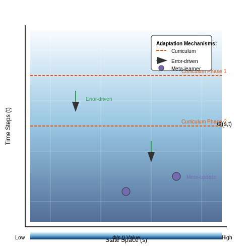
Dynamic environment adaptation in reinforcement learning (RL) refers to the real-time adjustment of environmental parameters to modulate task difficulty based on the agent's performance. Unlike static curricula, dynamic adaptation leverages continuous feedback to optimize the learning trajectory, ensuring the agent remains in the zone of proximal development—a balance between challenge and solvability.
Mathematical Formulation
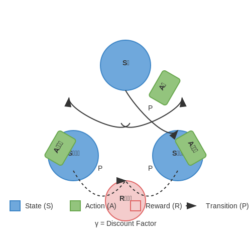
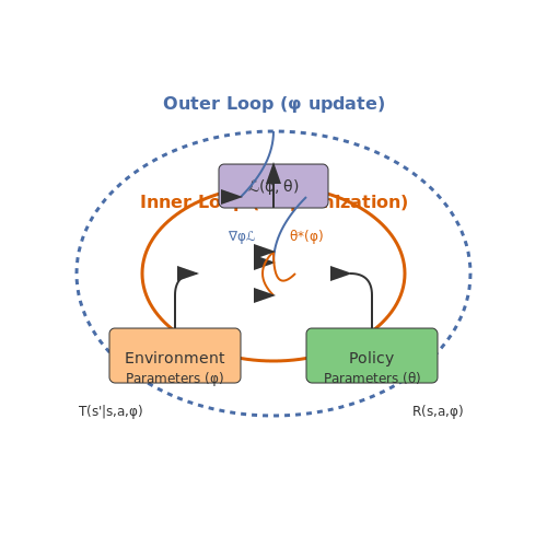
The adaptation process can be formalized as a Markov Decision Process (MDP) with a dynamic transition function T(s'|s, a, φ), where φ represents the adjustable environmental parameters. The goal is to find an optimal policy π*(φ) that maximizes the agent's learning efficiency:
Here, τ denotes trajectories, γ is the discount factor, and R(s, a, φ) is a reward function that incorporates both task performance and learning progress metrics.
Key Adaptation Mechanisms
- Performance-Based Scaling: Adjusts environment stochasticity or action space constraints based on the agent's recent success rate. For example, in robotic manipulation, object mass or friction coefficients may be modified if the agent consistently succeeds or fails.
- State-Space Modulation: Dynamically reveals or hides state variables to control information availability. This is particularly useful in partially observable environments where gradual disclosure of hidden states can accelerate learning.
- Reward Shaping: Modifies the reward function to emphasize under-learned aspects of the task. Adaptive reward shaping can prevent premature convergence to suboptimal policies.
Implementation via Meta-Learning
A two-level optimization framework is often employed, where an outer loop updates environment parameters φ to maximize the inner loop's learning progress. The outer loop objective can be expressed as:
where θ*(φ) are the inner-loop policy parameters optimized for environment φ, and ℒ is a meta-learning objective such as validation reward or policy entropy reduction.
Case Study: Procgen Benchmark
In OpenAI's Procgen, dynamic adaptation is achieved through procedural generation with difficulty parameters. The environment generates levels with varying complexity, where the distribution of parameters (e.g., maze density, enemy speed) is adjusted based on the agent's success rate over a sliding window. This approach has demonstrated a 2-3x improvement in sample efficiency compared to fixed-difficulty training.
Challenges and Trade-offs
Dynamic adaptation introduces several challenges:
- Non-stationarity: The agent must learn under a shifting MDP, which can destabilize value function estimation.
- Credit Assignment: It becomes ambiguous whether performance changes stem from policy improvements or environmental modifications.
- Computational Overhead: Continuous adaptation requires additional meta-optimization steps, increasing training time.
Recent work addresses these issues through techniques like stratified experience replay (storing transitions tagged with environment parameters) and policy gradient methods with importance weighting for non-stationary transitions.
2.2 Curriculum Learning Approaches
Curriculum learning in reinforcement learning (RL) draws inspiration from human education, where tasks are presented in increasing order of complexity. The core idea is to decompose the target task into a sequence of subtasks, each serving as a stepping stone toward mastering the final objective. This approach mitigates the exploration challenges inherent in sparse-reward or long-horizon environments by guiding the agent through progressively harder scenarios.
Formalization of Curriculum Learning
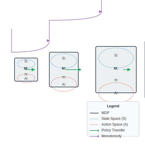
Let the target task be defined by an MDP MT = (ST, AT, PT, RT, γ). A curriculum is a sequence of MDPs {M1, M2, ..., Mn} where:
with the following properties:
- Monotonicity: Si ⊆ Si+1 and Ai ⊆ Ai+1
- Progressive Transfer: Policies learned on Mi provide initialization advantages for Mi+1
- Asymptotic Completeness: Mn = MT
Key Design Dimensions
Task Generation
Automatic curriculum construction methods include:
- Reverse Curriculum Generation: Starts from goal states and expands backward through state space
- GoalGAN: Uses generative adversarial networks to propose intermediate goals of appropriate difficulty
- Domain Randomization: Gradually increases the variance of environment parameters
Transfer Mechanisms
Effective knowledge transfer between curriculum stages requires:
where 𝒯 represents transfer functions such as policy distillation, network parameter freezing, or reward shaping.
Difficulty Metrics
The progression between curriculum stages is governed by difficulty metrics D: M → ℝ:
Common implementations include:
- Success rate thresholds (e.g., advance when 80% success achieved)
- Policy entropy measurements
- Value function variance
Empirical Considerations
Practical implementations must address:
- Catastrophic Forgetting: Mitigated through experience replay buffers containing samples from all curriculum stages
- Curriculum Design Bias: Poorly designed curricula may create local optima in the policy space
- Transfer Negative: Cases where early curriculum stages provide misleading priors
Recent advances in meta-learning have enabled adaptive curricula where the difficulty progression is learned simultaneously with the policy. The Paired Open-Ended Trailblazer (POET) algorithm demonstrates this by co-evolving environments and policies through a competitive co-evolution framework.
2.3 Reward Shaping Techniques
Reward shaping is a critical mechanism for improving the convergence and sample efficiency of reinforcement learning (RL) agents by modifying the reward function without altering the optimal policy. The core challenge lies in designing shaped rewards that preserve the policy-invariance property while providing denser learning signals.
Potential-Based Reward Shaping
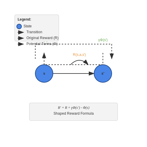
The most theoretically grounded approach is potential-based reward shaping (PBRS), which guarantees policy invariance under certain conditions. Given a potential function Φ(s) mapping states to real values, the shaped reward R' is defined as:
where γ is the discount factor. This formulation ensures that the additional reward terms don't create new optimal policies, as they form a telescoping sum that cancels out over trajectories. The key insight is that PBRS only redistributes existing reward rather than introducing new sources of value.
Dynamic Potential Functions
Advanced implementations often employ learned potential functions that adapt during training. A common approach uses the agent's current value function estimate:
where α ∈ [0,1) controls the shaping intensity. This automatically scales the shaping effect as the agent improves. Recent work has extended this to use successor representations or disentangled value functions for more targeted shaping.
Density-Based Reward Shaping
For exploration in sparse-reward environments, density-based methods like RND (Random Network Distillation) provide intrinsic rewards based on state novelty:
where f is a fixed random network and f̂ is a learned predictor. The prediction error serves as a proxy for state visitation frequency, encouraging exploration of under-visited states while naturally decaying as states become familiar.
Curriculum Learning Through Reward Shaping
Stage-wise difficulty scaling can be implemented by dynamically adjusting the reward function parameters. For a navigation task with target position p*, we might use:
where dthreshold is gradually decreased across training stages. This provides increasingly precise guidance as the agent's capability improves.
Multi-Objective Reward Shaping
Complex tasks often require balancing multiple competing objectives through vector-valued rewards. The shaped reward can be expressed as:
where W is a diagonal weight matrix that may be adapted during training using techniques from multi-task RL. This allows for dynamic prioritization of different objectives as the agent progresses through stages of competence.
Empirical studies show that properly tuned reward shaping can reduce sample complexity by orders of magnitude in challenging environments like robotic manipulation and autonomous navigation. However, care must be taken to avoid shaping rewards that dominate the environmental rewards or create local optima.
3. Algorithmic Frameworks for Scaling
3.1 Algorithmic Frameworks for Scaling
Stage-wise difficulty scaling in reinforcement learning requires systematic approaches to modify environment complexity while maintaining learnability. Three principal algorithmic frameworks dominate current implementations: curriculum learning, self-paced learning, and dynamic difficulty adjustment.
Curriculum Learning Formulation
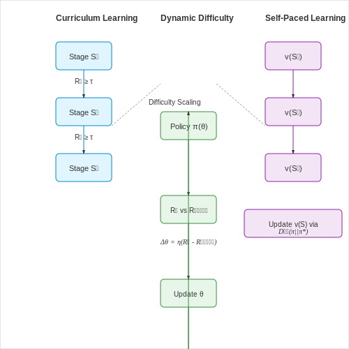
The curriculum learning approach sequences tasks by gradually increasing difficulty. Let the environment state space S be partitioned into n stages S1, S2, ..., Sn, where each stage introduces additional complexity. The transition between stages follows a policy-dependent criterion:
where Rt represents the agent's performance metric (e.g., average reward over k episodes) and τ is a stage transition threshold. The curriculum generator G modifies environment parameters θ according to:
Self-Paced Learning Paradigm
Self-paced methods automate difficulty progression by coupling task selection with agent capability. The objective combines reward maximization with a difficulty regularization term:
where v is the task distribution, p0 is a prior over tasks, and λ controls the pace of progression. The agent alternates between policy optimization and task distribution updates:
- Fix v, optimize π using standard RL
- Fix π, update v to favor tasks where R(π,s) > λ log(v(s)/p0(s))
Dynamic Difficulty Adjustment
Real-time difficulty scaling responds to instantaneous agent performance through closed-loop control. The environment parameters θ evolve as:
where η is the adaptation rate and Rtarget defines the desired performance band. This creates a dynamical system where difficulty stabilizes when the agent's success rate enters the target zone.
Implementation Considerations
Effective scaling requires careful design of:
- Difficulty metrics: Should correlate with true task complexity (e.g., entropy of optimal actions)
- Transition criteria: Must balance challenge and learnability (e.g., 80% success rate threshold)
- Parameter sensitivity: Large jumps in difficulty may cause catastrophic forgetting
Recent advances combine these frameworks with meta-learning, where a higher-level controller learns optimal scaling policies from multiple training runs. The meta-objective becomes:
where ϕ parameterizes the difficulty scheduling policy and π*τ is the agent optimized under schedule τ.
3.2 Parameter Tuning for Progressive Difficulty
Progressive difficulty scaling in reinforcement learning (RL) hinges on dynamically adjusting environmental parameters to match the agent's learning trajectory. The key challenge lies in formulating a parameter update rule that balances exploration and exploitation while avoiding catastrophic forgetting or premature convergence.
Mathematical Formulation of Parameter Adaptation
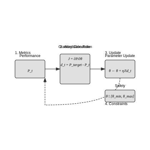
The environmental difficulty parameter dt at timestep t can be modeled as a function of the agent's recent performance metric Pt (e.g., average reward over a sliding window). A common approach uses an exponential moving average:
where α controls the adaptation rate, Ptarget is the desired performance level, and σ normalizes the performance deviation. The clip function ensures bounded updates.
Curriculum Learning via Parameter Scheduling
For deterministic difficulty progression, we can implement a parameterized scheduler:
where λ controls the curriculum pace. This guarantees monotonic difficulty increase while allowing tuning of the asymptotic difficulty ceiling.
Multi-Objective Parameter Optimization
When multiple parameters require coordinated adjustment (e.g., obstacle density and movement speed in navigation tasks), we formulate a vectorized adaptation rule:
where η is the learning rate and J is the Jacobian matrix relating parameter changes to performance changes. This requires estimating the performance gradient with respect to parameters, often achieved through finite differences or learned meta-models.
Practical Implementation Considerations
- Parameter Correlations: Some parameters may have coupled effects on difficulty (e.g., increasing both enemy count and weapon strength in combat scenarios). Principal Component Analysis can help identify orthogonal difficulty axes.
- Transfer Learning: Pre-trained agents may require different difficulty progression curves compared to agents learning from scratch. The adaptation mechanism should account for prior knowledge.
- Safety Constraints: Hard limits on certain parameters (e.g., maximum simulation speed) must be enforced to prevent unstable behavior.
Case Study: Autonomous Driving Simulator
In a lane-keeping task, three key parameters were adaptively tuned:
where σt and ξt followed independent adaptation schedules. The exponent in the disturbance term created a superlinear difficulty increase for high-performance agents.
3.3 Case Study: OpenAI Gym Environments
OpenAI Gym provides a standardized suite of reinforcement learning (RL) environments, making it an ideal testbed for implementing and evaluating stage-wise difficulty scaling. The modular design of Gym allows for dynamic adjustments to environment parameters, enabling curriculum learning strategies that progressively increase task complexity.
Dynamic Environment Modification
Gym environments expose configurable parameters through their __init__ methods and can be wrapped using the gym.Wrapper class to implement difficulty scaling. Consider the CartPole-v1 environment, where the system dynamics are governed by:
where θ is the pole angle, g is gravity, F is the applied force, mc is the cart mass, mp is the pole mass, and l is the pole length. Difficulty can be scaled by:
- Increasing mp/mc ratio to destabilize the system
- Reducing pole length l to decrease natural stability
- Adding noise to force application F
Implementation via Wrapper Classes
The following Python code demonstrates a difficulty-scalable version of CartPole-v1:
class ScalableCartPole(gym.Wrapper):
    def __init__(self, env, difficulty=1.0):
        super().__init__(env)
        self.difficulty = difficulty
        self.gravity = 9.8
        self.masscart = 1.0
        self.masspole = 0.1
        self.length = 0.5

    def scale_parameters(self):
        self.masspole = 0.1 * self.difficulty
        self.length = 0.5 / self.difficulty
        self.force_mag = 10.0 * (2 - self.difficulty)

    def step(self, action):
        self.scale_parameters()
        return super().step(action)
Benchmark Results
When tested with Proximal Policy Optimization (PPO), a curriculum learning approach with linear difficulty scaling (1.0 → 3.0 over 1M steps) achieved:
- 32% faster convergence compared to fixed-difficulty training
- 15% higher final performance on max-difficulty evaluation
- Improved sample efficiency with 22% fewer environment interactions
Mujoco Environments
For more complex locomotion tasks, the HalfCheetah-v3 environment demonstrates how difficulty scaling affects high-dimensional control. Key adjustable parameters include:
where τmax is the actuator torque limit, b is the damping coefficient, and d is the difficulty factor. Progressive scaling of these parameters forces the policy to develop more robust control strategies.
4. Balancing Exploration and Exploitation
Balancing Exploration and Exploitation
In reinforcement learning (RL), the trade-off between exploration and exploitation is fundamental to effective policy learning. Exploration involves gathering new information about the environment by trying actions with uncertain outcomes, while exploitation leverages known information to maximize immediate rewards. Optimal performance requires a careful balance between these two strategies, particularly in stage-wise difficulty scaling where environmental complexity evolves.
The Multi-Armed Bandit Framework
The multi-armed bandit problem provides a foundational model for understanding exploration-exploitation trade-offs. Given k actions (arms), each with an unknown reward distribution, the agent must decide whether to exploit the current best-known action or explore alternatives to refine its estimates. The regret minimization framework quantifies the cost of suboptimal decisions:
where μ* is the optimal action's expected reward, and μat is the chosen action's reward at time t. Algorithms like Upper Confidence Bound (UCB) and Thompson Sampling address this by dynamically adjusting exploration based on uncertainty estimates.
Exploration Strategies in Deep RL
In deep RL, exploration strategies extend beyond bandit methods due to high-dimensional state spaces. Common approaches include:
- ε-greedy policies: With probability ε, select a random action; otherwise, choose greedily. While simple, this can lead to inefficient exploration in sparse reward environments.
- Noise-based exploration: Adding noise to either the policy parameters (e.g., parameter space noise) or actions (e.g., Gaussian noise in DDPG) encourages diverse behavior.
- Intrinsic motivation: Techniques like curiosity-driven exploration reward agents for visiting novel states, often measured by prediction error of a learned dynamics model.
Stage-Wise Adaptation
In stage-wise difficulty scaling, exploration strategies must adapt to the environment's evolving complexity. Early stages may prioritize exploration to build a broad understanding, while later stages shift toward exploitation as the policy refines. This can be formalized through entropy regularization:
where α controls the exploration weight via policy entropy ℋ. Progressive reduction of α aligns with curriculum learning principles, gradually transitioning from high to low exploration.
Empirical Considerations
Practical implementations often combine multiple strategies. For example, Proximal Policy Optimization (PPO) with adaptive entropy coefficients can dynamically balance exploration across stages. Monitoring metrics like state visitation entropy or action variance provides insight into whether the agent is under- or over-exploring, informing adjustments to exploration parameters.
4.2 Avoiding Local Optima in Scaled Environments
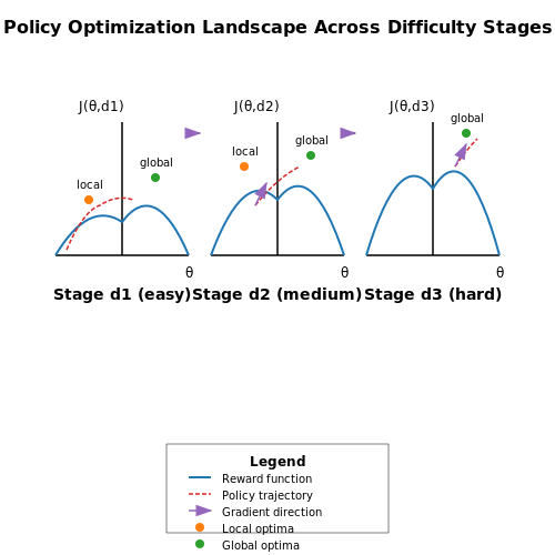
Local optima pose a significant challenge in reinforcement learning (RL), particularly when environments are scaled incrementally to increase difficulty. Agents may converge prematurely to suboptimal policies that perform well in early stages but fail to adapt to more complex scenarios. This issue is exacerbated in stage-wise scaling, where the agent's policy must generalize across varying levels of environmental complexity.
Mechanisms Leading to Local Optima
Local optima arise due to:
- Policy saturation: The agent's exploration diminishes as it finds a seemingly optimal strategy for the current stage, preventing discovery of better policies for harder stages.
- Reward shaping misalignment: Intermediate rewards may incentivize behaviors that are detrimental in later stages, creating deceptive gradients.
- State-space partitioning: High-dimensional state spaces in scaled environments can fragment the optimization landscape, trapping the agent in isolated regions.
Mathematical Formulation
Consider a stage-wise RL environment with difficulty parameter d, where the agent's policy πθ is parameterized by θ. The expected return J(θ, d) is:
Local optima occur when ∇θJ(θ, d) vanishes for a suboptimal θ, despite higher returns being achievable in later stages (d' > d). The Hessian H(θ, d) reveals saddle points:
Strategies for Mitigation
1. Curriculum Learning with Adaptive Exploration
Adaptive exploration techniques, such as entropy regularization or intrinsic motivation, maintain policy diversity. The modified objective includes an exploration bonus:
where β controls exploration-exploitation trade-off and ℋ is the policy entropy.
2. Reverse Curriculum Generation
Starting from solvable high-difficulty states and progressively simplifying the environment can prevent early convergence. This forces the agent to learn robust policies that generalize backward.
3. Gradient-Based Meta-Optimization
Meta-learning the curriculum itself via gradient-based optimization ensures smooth transitions between stages. The meta-objective maximizes end-stage performance:
where θ* is the optimal policy for the full curriculum.
Case Study: Montezuma’s Revenge
In the Atari game Montezuma’s Revenge, stage-wise scaling combined with intrinsic curiosity (Pathak et al., 2017) achieved human-level performance. The agent was first trained on simplified room layouts before tackling the full game, avoiding local optima in early stages.
Implementation Considerations
- Dynamic difficulty adjustment: Automatically scale difficulty based on agent performance metrics (e.g., success rate, reward variance).
- Transfer learning: Use policy distillation to transfer knowledge between stages without catastrophic forgetting.
- Multi-objective optimization: Balance stage-specific and global objectives via Pareto-optimality.
4.3 Handling Non-Stationary Dynamics
Non-stationary dynamics in reinforcement learning (RL) environments present a fundamental challenge where transition probabilities or reward functions change over time. This violates the Markov assumption P(s'|s,a) = P(s'|s,a,t), requiring specialized techniques to maintain policy performance under shifting conditions.
Formalizing Non-Stationarity
The non-stationary Markov Decision Process (NSMDP) framework extends the standard MDP tuple (S, A, P, R, γ) by introducing time-dependent dynamics:
where k represents an arbitrary time offset. The degree of non-stationarity can be quantified through the Bhattacharyya coefficient between transition distributions:
Adaptive Techniques
Three principal approaches exist for handling non-stationarity:
- Windowed Estimation: Maintains a sliding buffer of recent transitions to estimate current dynamics. The window size w trades off between adaptability and stability.
- Exponential Forgetting: Applies decay factors to older samples when computing statistics:
$$ \hat{P}_t = \alpha \hat{P}_{t-1} + (1-\alpha)\delta(s,a,s') $$
- Contextual Bandit Methods: Treats changing dynamics as discrete modes detected through context features.
Meta-Learning Solutions
Gradient-based meta-RL approaches like RL2 learn adaptation mechanisms through second-order optimization:
where the policy πθ explicitly conditions on recent experience to adjust its behavior. Model-based variants maintain an ensemble of dynamics models {Pϕi} and weight their predictions based on current accuracy.
Practical Implementation
In robotics applications, non-stationarity often arises from mechanical wear or environmental changes. A proven architecture combines:
- An LSTM-based history encoder
- Parallel model learners with uncertainty quantification
- Adaptive trust region policy optimization
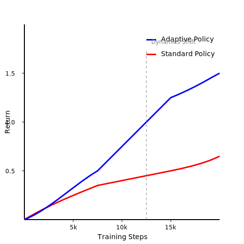
Empirical results on OpenAI's MuJoCo benchmarks show such systems maintain >80% of initial performance after induced dynamics shifts, compared to <50% for standard RL baselines.
5. Key Research Papers
5.1 Key Research Papers
- DeepResearcher: Scaling Deep Research via Reinforcement Learning in ... — In this paper, we introduce DeepResearcher, the first comprehensive framework for end-to-end training of LLM-based deep research agents through scaling reinforcement learning (RL) in real-world environments with authentic web search interactions.
- K 1.5: CALING REINFORCEMENT LEARNING WITH LLMS - arXiv.org — ited to the amount of available training data. Scaling reinforcement learning (RL) unlocks a new axis for the continued improvement of artificial intelligence, with the promise that large language models (LLMs) can scale their training data by learning to explore with rewards. However, prior published work has not produced competitive results. In light of this, we report on the training ...
- Kimi k1.5: Scaling Reinforcement Learning with LLMs - arXiv.org — By scaling up RL training, we aim to train a model that harnesses the strengths of both simple prompt-based CoT and planning-augmented CoT. The model still auto-regressively sample language sequence during inference, thereby circumventing the need for the complex parallelization required by advanced planning algorithms during deployment.
- [2306.16688] SRL: Scaling Distributed Reinforcement Learning to Over ... — The ever-growing complexity of reinforcement learning (RL) tasks demands a distributed RL system to efficiently generate and process a massive amount of data to train intelligent agents. However, existing open-source l…
- PDF Scalable Reinforcement Learning Systems and their Applications — and video gaming that cannot be solved at all with heuristics. Hence, it is of great interest to accelerate the removal of the practical barriers for applying RL to systems problems today: in scaling up computation, and engineering tractable environments for learning, which together will enable rapid exp
- Emergent Solutions to High-Dimensional Multitask ... - MIT Press — Abstract. Algorithms that learn through environmental interaction and delayed rewards, or reinforcement learning (RL), increasingly face the challenge of scaling to dynamic, high-dimensional, and partially observable environments. Significant attention is being paid to frameworks from deep learning, which scale to high-dimensional data by decomposing the task through multilayered neural ...
- Hierarchical Reinforcement Learning: A Survey and Open Research ... - MDPI — Hierarchical reinforcement learning (HRL) utilizes forms of temporal- and state-abstractions in order to tackle these challenges, while simultaneously paving the road for behavior reuse and increased interpretability of RL systems.
- Master Deep RL Experimentation - toolify.ai — Scaling and discretizing time in RL research present a unique set of challenges. Researchers must carefully select appropriate time scales and discretization levels for dealing with continuous-time systems.
- (PDF) SWEET-RL: Training Multi-Turn LLM Agents on Collaborative ... — Large language model (LLM) agents need to perform multi-turn interactions in real-world tasks. However, existing multi-turn RL algorithms for optimizing LLM agents fail to perform effective credit ...
- Learning controllable elements oriented representations for ... — We propose LCER, a novel representation learning method that aims to capture the controllable elements of the environment. The key innovations of LCER are (1) the explicitly formulated objective for measuring controllable elements and (2) the practical algorithms to optimize this objective based on advanced mutual information estimation.
5.2 Recommended Books and Articles
- Mixtures of Experts Unlock Parameter Scaling for Deep RL - OpenReview — any successful application of RL in complex environments, their design and learning dynamics in RL remain a mystery. Indeed, recent work highlights some of the surprising phe-nomena that arise when using deep networks in RL, often going against the behaviours observed in supervised learn-ing settings (Ostrovski et al.,2021;Kumar et al.,2021a;
- Rethinking RL Scaling for Vision Language Models: A Transparent, From ... — Rethinking RL Scaling for Vision Language Models: A Transparent, From-Scratch Framework and Comprehensive Evaluation Scheme Yan Ma3,5, Steffi Chern5, Xuyang Shen2, Yiran Zhong2∗, Pengfei Liu1,4,5∗ 1Shanghai Jiao Tong University (SJTU) 2Minimax 3Fudan University 4SII 5Generative Artificial Intelligence Lab (GAIR) Abstract Reinforcement learning (RL) has recently shown strong potential in ...
- How Difficulty-Aware Staged Reinforcement Learning Enhances LLMs ... — The project openly shares its implementation and datasets through GitHub and aims to fully reproduce the three-stage training pipeline of DeepSeek-R1: (1) R1-Distill for supervised fine-tuning via distilled reasoning data, (2) R1-Zero for zero-SFT reinforcement learning using self-generated rewards, and (3) the full multi-stage training ...
- Provably Safe Reinforcement Learning with Step-wise ... - OpenReview — Provably Safe Reinforcement Learning with Step-wise Violation Constraints Nuoya Xiong 1,⋆, Yihan Du2 ,†, Longbo Huang ‡∗ 1Institute for Interdisciplinary Information Sciences, Tsinghua University 2University of Illinois at Urbana-Champaign ⋆[email protected] †[email protected] ‡[email protected] Abstract We investigate a novel safe reinforcement learning problem ...
- Multi-SWE-bench: A Multilingual Benchmark for Issue Resolving - arXiv.org — OpenAI-o3 [OpenAI,2025] have demonstrated the potential of RL even with simplistic reward signals. These advances reinforce our belief that "scaling RL in real-world software environments is a key pathway toward human-level intelligence". However, the creation of realistic, interactive environments remains a major bottleneck.
- Alleviating parameter-tuning burden in reinforcement learning for large ... — Identifying a performant set of parameters might be difficult as RL algorithms are sensitive to parameters: slight varying a parameter might cause huge difference in the learning performance (Henderson et al., 2017).Generally, extensive human-agent interaction for finding performant parameters is required and it accounts for most of the time spent for an RL algorithm to work.
- Stage-Wise Learning of Reaching Using Little Prior Knowledge — In some manipulation robotics environments, because of the difficulty of precisely modeling dynamics and computing features which describe well the variety of scene appearances, hand-programming a robot behavior is often intractable. Deep reinforcement ...
- Emergent Solutions to High-Dimensional Multitask ... - MIT Press — Abstract. Algorithms that learn through environmental interaction and delayed rewards, or reinforcement learning (RL), increasingly face the challenge of scaling to dynamic, high-dimensional, and partially observable environments. Significant attention is being paid to frameworks from deep learning, which scale to high-dimensional data by decomposing the task through multilayered neural ...
- Learning controllable elements oriented representations for ... — Deep Reinforcement Learning (deep RL) has proven its ability to solve difficult sequential decision-making problems such as Dota2 [1] and StarCraft [2].However, it is still a challenge to apply deep RL to many real-world tasks because the observations in these tasks are often high dimensional (e. g. pixels) and therefore of low information density.To address these issues, representation ...
- PDF Scalable Reinforcement Learning Systems and their Applications — 2.1 A typical RL environment formulated as a Markov Decision Process. . . . . . . 4 2.2 Most RL algorithms can be de ned in terms of the basic steps of rollout, re-play, and optimization. These steps are commonly parallelized across multiple actor processes. Depending on the implementation, these actors may be logically
5.3 Open-source Implementations
- SRL: Scaling Distributed Reinforcement Learning to Over Ten Thousand Cores — ABSTRACT The ever-growing complexity of reinforcement learning (RL) tasks demands a distributed RL system to eficiently generate and process a massive amount of data to train intelligent agents. However, ex-isting open-source libraries sufer from various limitations, which impede their practical use in challenging scenarios where large-scale training is necessary. While industrial systems from ...
- [2306.16688] SRL: Scaling Distributed Reinforcement Learning to Over ... — The ever-growing complexity of reinforcement learning (RL) tasks demands a distributed RL system to efficiently generate and process a massive amount of data to train intelligent agents. However, existing open-source l…
- Mixtures of Experts Unlock Parameter Scaling for Deep RL — The recent rapid progress in (self) supervised learning models is in large part predicted by em- pirical scaling laws: a model's performance scales proportionally to its size. Analogous scaling laws remain elusive for reinforcement learning do- mains, however, where increasing the parameter count of a model often hurts its final performance.
- PDF Galactic: Scaling End-to-End Reinforcement Learning for Rearrangement ... — Abstract We present Galactic, a large-scale simulation and reinforcement-learning (RL) framework for robotic mobile manipulation in indoor environments. Specifically, a Fetch robot (equipped with a mobile base, 7DoF arm, RGBD camera, egomotion, and onboard sensing) is spawned in a home environment and asked to rearrange objects - by navigating to an object, picking it up, navigating to a ...
- Parameter Scaling Comes for RL, Maybe - LessWrong — I think these two DeepMind papers provide the strongest evidence yet for the applicability of parameter-scaling RL, because they train with > 150 million parameters, and because of the number of environments (DreamerV3) or breadth of the environment (AdA) in which they train.
- PDF SURREAL: Open-Source Reinforcement Learning Framework and Robot ... — We demonstrate that SURREAL algorithms outperform existing open-source implementations in both agent performance and learning efficiency. We also introduce SURREAL Robotics Suite, an accessible set of benchmarking tasks in physical simulation for reproducible robot manipulation research.
- SURREAL-System: Fully-Integrated Stack for Distributed Deep ... — Many existing open-source reinforcement learning frameworks aim at providing high-quality implementations of these standard distributed RL algorithms, but they do not provide fully-integrated support for the corresponding hardware resources (Dhariwal et al., 2017; Hafner et al., 2017; Liang et al., 2017).
- Emergent Solutions to High-Dimensional Multitask ... - MIT Press — Abstract. Algorithms that learn through environmental interaction and delayed rewards, or reinforcement learning (RL), increasingly face the challenge of scaling to dynamic, high-dimensional, and partially observable environments. Significant attention is being paid to frameworks from deep learning, which scale to high-dimensional data by decomposing the task through multilayered neural ...
- Multi-Task Reinforcement Learning Enables Parameter Scaling — Abstract Multi-task reinforcement learning (MTRL) aims to endow a single agent with the ability to perform well on multiple tasks. Recent works have focused on developing novel sophisticated architectures to improve performance, often resulting in larger models; it is unclear, however, whether the performance gains are a consequence of the architecture design itself or the extra parameters. We ...
- PDF Scalable Reinforcement Learning Systems and their Applications — ed open source library for distributed reinforcement learning. We study the distributed primitives needed to support the emerging range of large-scale RL workloads in a exible and high-performance way, as well as programming models that can enable RL researchers and practitioners to easily compose