StyleGAN2 and Style Transfer Techniques
1. Core Architecture of GANs
Core Architecture of GANs
Adversarial Training Framework
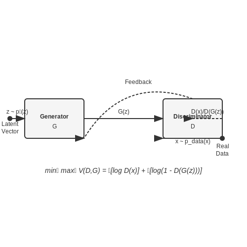
The foundational architecture of Generative Adversarial Networks (GANs) consists of two neural networks—the generator (G) and the discriminator (D)—engaged in a minimax game. The generator learns to map latent noise vectors z to synthetic data samples, while the discriminator distinguishes between real data x and generated samples G(z). The adversarial objective is formalized as:
Here, pdata(x) represents the real data distribution, and pz(z) is the prior noise distribution (typically Gaussian or uniform). The discriminator outputs a probability score between 0 (fake) and 1 (real).
Network Architectures
In deep convolutional GANs (DCGANs), both G and D employ strided convolutions and transposed convolutions:
- Generator: Upsamples latent vectors via transposed convolutions, batch normalization, and ReLU/LeakyReLU activations.
- Discriminator: Uses convolutional layers with spectral normalization for stability, followed by LeakyReLU and dropout.
Loss Functions and Training Dynamics
The vanilla GAN suffers from mode collapse and vanishing gradients. Improved variants use alternative loss functions:
Wasserstein GANs (WGANs) replace the Jensen-Shannon divergence with Earth-Mover distance, enforced via Lipschitz constraints. StyleGAN2 further refines this with path length regularization to disentangle latent space.
Latent Space Manipulation
GANs project noise z into an intermediate latent space W through learned affine transformations. StyleGAN2’s mapping network f: Z → W enables hierarchical style control via adaptive instance normalization (AdaIN):
where ys, yb are style vectors modulating feature statistics at layer i.
Practical Challenges
Training instability arises from:
- Gradient competition: D and G must evolve at balanced rates.
- Mode collapse: G generates limited sample diversity.
- Evaluation metrics: Fréchet Inception Distance (FID) and Precision/Recall for distributions quantify performance.
1.2 Training Dynamics and Challenges
Training Dynamics in StyleGAN2
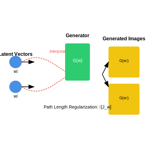
StyleGAN2 improves upon its predecessor by addressing key training instabilities through architectural modifications. The generator employs a path length regularization term to ensure smoother latent space interpolations, defined as:
where Jw is the Jacobian of the generator output with respect to the latent code w, y is a random unit vector, and a is a dynamically updated exponential moving average of the path lengths. This regularization prevents mode collapse by penalizing abrupt changes in the generated images as the latent code varies.
Challenges in Training StyleGAN2
Despite its improvements, StyleGAN2 faces several challenges during training:
- Memory Constraints: The high-resolution synthesis (1024×1024) requires significant GPU memory, often necessitating gradient checkpointing or mixed-precision training.
- Training Time: Convergence can take days even on modern hardware due to the adversarial training paradigm and progressive growing.
- Latent Space Disentanglement: While StyleGAN2 improves disentanglement compared to StyleGAN, fine-grained control over specific attributes remains non-trivial.
Optimization Strategies
The adversarial loss function in StyleGAN2 combines the standard non-saturating GAN loss with R1 regularization for the discriminator:
Here, f(t) = -log(1 + exp(-t)) is the softplus function, and γ controls the strength of gradient penalty. The R1 regularization stabilizes training by penalizing large discriminator gradients on real data.
Empirical Observations
Several empirical findings influence successful training:
- Using equalized learning rates for all layers prevents signal magnitude issues in deep networks.
- The lazy regularization technique, where path length and R1 regularization are not computed every iteration, reduces computational overhead by 25-30%.
- Progressive growing, while not used in the final StyleGAN2, remains relevant for initializing high-resolution training.
Numerical Instabilities
StyleGAN2 is susceptible to numerical instabilities when:
where λmax is the maximum eigenvalue of the Jacobian. This manifests as "phase artifacts" in generated images, addressed in StyleGAN2-ADA through adaptive discriminator augmentation.
Evolution from GAN to StyleGAN
Foundational GAN Architecture
The original Generative Adversarial Network (GAN) framework, introduced by Goodfellow et al. in 2014, consists of two competing neural networks: a generator G and a discriminator D. The generator maps latent vectors z from a prior distribution (typically Gaussian) to synthetic data samples, while the discriminator attempts to distinguish between real and generated samples. The adversarial objective is formulated as:
Despite its theoretical elegance, early GANs suffered from training instability, mode collapse, and difficulty scaling to high-resolution images. The latent space z lacked interpretable controls over image attributes, limiting practical applications.
Progressive Growing and Style-Based Generation
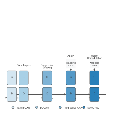
Progressive GAN (2017) introduced hierarchical generation by progressively increasing resolution during training, improving stability for high-resolution synthesis. StyleGAN (2018) revolutionized this approach by decoupling high-level attributes (pose, hairstyle) from stochastic details (freckles, hair strands) through:
- A learned affine transformation mapping latent z to intermediate latent space w
- Adaptive Instance Normalization (AdaIN) to inject style at each convolutional layer
- Explicit noise inputs for fine-grained stochastic variation
The generator architecture became:
StyleGAN2 Architectural Improvements
StyleGAN2 (2020) addressed artifacts like droplet-shaped distortions and phase inconsistencies by:
- Replacing progressive growing with a residual skip generator
- Modifying weight demodulation instead of AdaIN for style application
- Introducing path length regularization to encourage linear latent space interpolations
The revised style modulation becomes:
where si are style weights and ϵ prevents numerical instability. This enabled higher-quality synthesis with more disentangled latent controls.
Key Evolutionary Milestones
| Model | Innovation | Limitations Addressed |
|---|---|---|
| Vanilla GAN | Adversarial training framework | Basic synthesis capability |
| DCGAN | Convolutional architectures | Unstable training on images |
| Progressive GAN | Layer-wise resolution growth | High-resolution generation |
| StyleGAN | Style-based generation | Attribute disentanglement |
| StyleGAN2 | Weight demodulation, path regularization | Artifact reduction, latent linearity |
2. Key Innovations in StyleGAN2
Key Innovations in StyleGAN2
Architectural Improvements
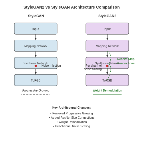
StyleGAN2 addresses several critical limitations of its predecessor by introducing architectural refinements that enhance both image quality and training stability. The most significant change is the removal of progressive growing, which was prone to introducing phase artifacts in generated images. Instead, StyleGAN2 employs a residual network (ResNet) inspired design, where skip connections allow gradients to flow more efficiently during backpropagation. This mitigates the vanishing gradient problem and stabilizes training for high-resolution outputs.
The generator now uses a weight demodulation technique instead of instance normalization, decoupling the style application from the noise inputs. This is mathematically expressed as:
where \( w_{ijk} \) are the original weights, \( \epsilon \) is a small constant for numerical stability, and \( w'_{ijk} \) are the demodulated weights. This ensures that the style modulation does not amplify noise artifacts.
Path Length Regularization
StyleGAN2 introduces a novel path length regularization term to encourage smoother latent space interpolations. The key insight is to penalize abrupt changes in the generator's output with respect to small perturbations in the latent space. The regularization term \( \mathcal{L}_{pl} \) is defined as:
Here, \( \mathbf{J}_{\mathbf{z}} \) is the Jacobian matrix of the generator output with respect to the latent code \( \mathbf{z} \), \( \mathbf{y} \) is a random unit vector, and \( a \) is a target scale hyperparameter. This term enforces consistent mapping distances in the latent space, reducing distortion in interpolated images.
Lazy Regularization
To improve computational efficiency, StyleGAN2 implements lazy regularization, where regularization terms (e.g., path length or R1 gradient penalty) are not computed at every training step. Instead, they are applied stochastically with a fixed probability, reducing the overhead while maintaining their benefits. This is particularly advantageous for large-scale training, where the discriminator's gradient penalty would otherwise dominate computation time.
Noise Input Redesign
The original StyleGAN applied per-pixel noise after each style modulation, which often led to droplet artifacts—localized high-frequency patterns. StyleGAN2 redefines noise injection by applying it to feature maps rather than individual pixels, with learned scaling factors per channel. This change is formalized as:
where \( \mathbf{F} \) is the feature map, \( \mathbf{b} \) is a learned per-channel scaling vector, and \( \mathbf{n} \) is spatially correlated noise. This results in more natural stochastic variations, such as realistic hair strands or skin pores.
Applications and Impact
These innovations collectively enable StyleGAN2 to generate higher-fidelity images with fewer artifacts, making it suitable for applications like synthetic dataset creation, facial reenactment, and artistic style transfer. For instance, NVIDIA's Face Synthesis demo leverages StyleGAN2's smooth latent space for photorealistic facial attribute editing, while research in medical imaging uses its stability to generate synthetic MRI scans for data augmentation.
Understanding Adaptive Instance Normalization (AdaIN)
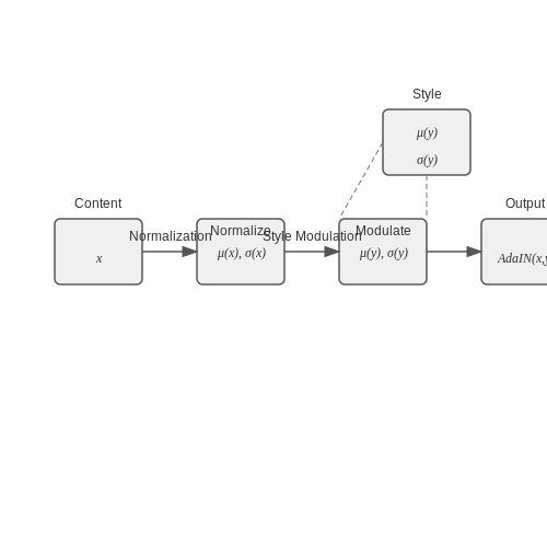
Adaptive Instance Normalization (AdaIN) is a critical component in StyleGAN2 and style transfer architectures, enabling the separation of content and style by dynamically aligning the mean and variance of feature maps. Unlike traditional instance normalization, which normalizes features independently for each sample and channel, AdaIN introduces style-dependent modulation by adapting normalization statistics from a style input.
Mathematical Formulation
Given a content input x and a style input y, AdaIN operates on the feature activations of x by first normalizing and then applying style-specific scaling and shifting. The operation is defined as:
where:
- μ(x) and σ(x) are the channel-wise mean and standard deviation of the content features.
- μ(y) and σ(y) are the corresponding style statistics, typically extracted from a style encoder or learned transformation.
Key Properties and Advantages
AdaIN's effectiveness stems from its ability to:
- Decouple style and content: By normalizing content features and applying style statistics, it ensures that high-level attributes (e.g., texture, color) are controlled independently of spatial structure.
- Enable arbitrary style transfer: The same content can be restyled by swapping y without retraining, as demonstrated in neural style transfer applications.
- Stabilize GAN training: In StyleGAN2, AdaIN replaces explicit noise injection, reducing artifacts by modulating features with learned style vectors.
Implementation Insights
In practice, AdaIN is implemented as a lightweight layer with no learnable parameters of its own. The style statistics μ(y) and σ(y) are typically generated by a multi-layer perceptron (MLP) from a latent style vector. For example, StyleGAN2's mapping network produces style codes that are transformed into modulation parameters for each convolutional layer.
import torch
import torch.nn as nn

class AdaIN(nn.Module):
    def __init__(self):
        super().__init__()

    def forward(self, x, y_mean, y_std):
        # Normalize content features
        x_mean = x.mean(dim=(2, 3), keepdim=True)
        x_std = x.std(dim=(2, 3), keepdim=True)
        x_normalized = (x - x_mean) / (x_std + 1e-8)

        # Apply style modulation
        return y_std * x_normalized + y_mean
Comparative Analysis with Other Normalization Techniques
AdaIN differs fundamentally from other normalization methods:
- Batch Normalization (BN): BN uses batch-level statistics, making it unsuitable for style transfer due to dependency on batch composition.
- Instance Normalization (IN): While IN normalizes individual samples, it lacks adaptive modulation, requiring additional style application layers.
- Conditional IN: Early approaches concatenated style features, but AdaIN's affine transformation proves more effective for disentangled representation learning.
Applications Beyond Style Transfer
AdaIN's versatility extends to:
- Domain adaptation: Aligning feature distributions between source and target domains without retraining.
- Image-to-image translation: Preserving content structure while altering domain-specific attributes in frameworks like FUNIT.
- Few-shot learning: Rapid adaptation to new classes by modulating feature statistics from few examples.
2.3 Noise Injection and Stochastic Variation
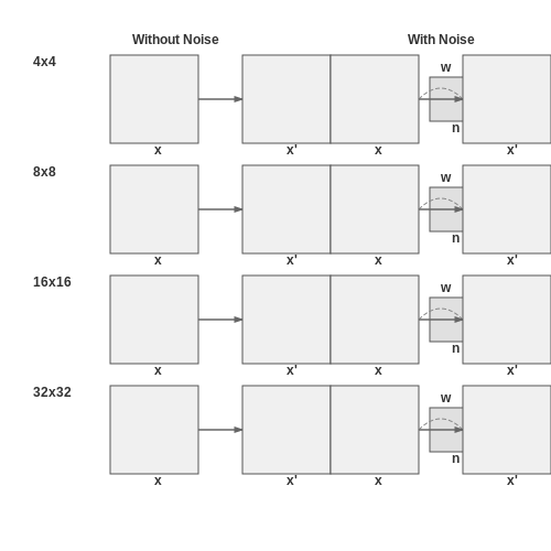
StyleGAN2 introduces stochastic variation through explicit noise injection at each layer of the generator network. Unlike traditional GANs, where noise is only provided at the input layer, StyleGAN2 applies per-pixel noise after each convolutional operation. This noise is modulated by learned scaling factors, allowing the network to control the degree of stochasticity at different resolutions.
Mathematical Formulation
The noise injection process can be formalized as follows. Let x be the feature map at a given layer, and n be a noise tensor sampled from a standard normal distribution. The modulated noise is applied as:
where w represents the learned per-channel scaling weights, and ⊙ denotes element-wise multiplication. The weights w are predicted by the style network, ensuring that noise application is style-adaptive.
Implementation Details
In practice, noise is injected after each convolutional layer in the synthesis network. The noise tensor n is broadcast to match the spatial dimensions of the feature map, while the scaling weights w are learned per feature channel. This design allows fine-grained control over stochastic effects:
- High-frequency details (e.g., hair strands, skin pores) are controlled by noise in early layers
- Global variations (e.g., lighting changes, pose shifts) are influenced by noise in deeper layers
Visual Effects of Noise Injection
The impact of noise injection can be visualized by examining generated samples with and without stochastic variation. Without noise, images appear overly smooth and lack fine details. With proper noise scaling, the generator produces realistic high-frequency features while maintaining coherent global structure. The figure below illustrates this effect across different resolutions:
Empirical Analysis
Quantitative evaluation reveals that proper noise scaling improves both the Fréchet Inception Distance (FID) and perceptual quality metrics. The optimal noise magnitude follows an inverse relationship with layer depth:
where wl is the noise weight at layer l, dl is the layer's depth (normalized to [0,1]), and α is a global scaling factor typically set between 0.1 and 0.3 through cross-validation.
Advanced Applications
Recent extensions have explored dynamic noise scheduling, where noise magnitudes are adjusted during training based on feature statistics. This adaptive approach helps balance detail generation with global coherence, particularly useful for high-resolution synthesis (1024×1024 and above). Some implementations also employ correlated noise patterns across spatial dimensions to model structured stochastic effects like fabric textures or wood grain.
Style Mixing and Hierarchical Latent Space
Hierarchical Latent Space in StyleGAN2
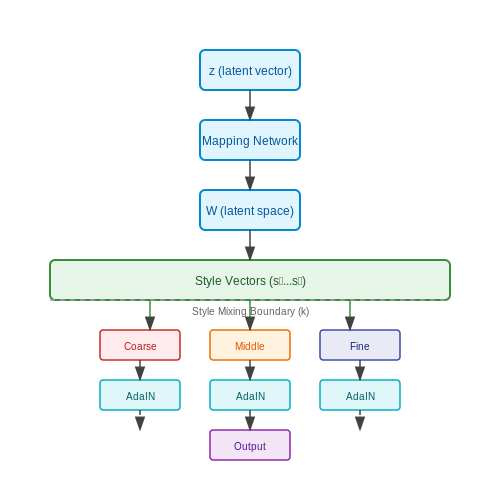
StyleGAN2 employs a hierarchical latent space structure where the input latent vector z is transformed into an intermediate latent space W through a learned mapping network. This space is then expanded into a set of style vectors s, which modulate the generator's convolutional layers via adaptive instance normalization (AdaIN). The hierarchical nature arises from the fact that different layers of the generator are controlled by different subsets of s, allowing coarse styles (e.g., pose, face shape) to affect early layers and fine styles (e.g., hair texture, skin details) to influence later layers.
where Ai represents the affine transformation for the i-th layer, and wi is the corresponding segment of the intermediate latent code.
Style Mixing Mechanism
Style mixing is a technique where two latent vectors z1 and z2 are used to generate an image by applying different segments of their respective style vectors to different layers of the generator. The crossover point determines the boundary between coarse and fine attributes. Mathematically, this is expressed as:
where k is the crossover layer index. This allows explicit control over which hierarchical level of style is inherited from each input.
Practical Applications and Implications
Style mixing enables fine-grained control over synthesized images, making it invaluable for applications like:
- Controlled image editing: Swapping high-level attributes (e.g., gender) while preserving low-level details (e.g., background).
- Data augmentation: Generating diverse training samples by recombining styles from different source images.
- Artistic style transfer: Blending stylistic elements from multiple references into a single output.
Mathematical Analysis of Disentanglement
The hierarchical structure promotes disentanglement by minimizing mutual information between style vectors at different levels. The loss function includes a term to enforce orthogonality in the learned style directions:
Empirical studies show this reduces unintended correlations between attributes (e.g., hair color and lighting conditions).
Visualization of Hierarchical Effects
The impact of style mixing can be visualized by progressively increasing the crossover point k from early to late layers. Early crossovers (e.g., layer 4) show dramatic changes in global structure, while later crossovers (e.g., layer 12) affect only localized textures. This demonstrates the spatial frequency separation learned by the generator's architecture.
3. Neural Style Transfer: Principles and Methods
Neural Style Transfer: Principles and Methods
Foundations of Neural Style Transfer
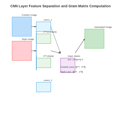
Neural Style Transfer (NST) redefines image synthesis by decoupling content and style representations using deep convolutional neural networks (CNNs). The core insight stems from the observation that different layers in a CNN capture distinct hierarchical features: lower layers encode fine-grained textures and colors (style), while higher layers extract semantic content and object structures. This separation enables the transfer of artistic style from one image to another while preserving the underlying content.
The mathematical formulation involves optimizing a generated image G to minimize two loss terms:
where α and β are weighting hyperparameters. The content loss Lcontent measures the Euclidean distance between feature maps of the content image C and generated image G at layer l in a pretrained VGG network:
Here, Fl and Pl represent the feature maps of G and C at layer l, respectively.
Gram Matrices for Style Representation
Style loss computation relies on Gram matrices, which capture feature correlations across different channels of a CNN layer. For a given layer l with Nl filters producing feature maps of size Ml = height × width, the Gram matrix Gl ∈ ℝNl × Nl is computed as:
The style loss then compares Gram matrices of the style image S and generated image G across multiple layers L:
where Al is the Gram matrix of the style image and wl are layer-specific weights.
Optimization Techniques
Modern NST implementations employ several optimizations beyond the original formulation:
- Total Variation Regularization: Penalizes high-frequency noise in the generated image using the anisotropic loss term:
$$ \mathcal{L}_{TV} = \sum_{i,j} \left( (G_{i,j+1} - G_{i,j})^2 + (G_{i+1,j} - G_{i,j})^2 \right) $$
- Multi-scale Processing: Applies style transfer at different resolutions to capture both global and local patterns
- Histogram Matching: Aligns color distributions between style and content images before optimization
Architectural Advancements
Recent variants improve upon the basic VGG-based approach:
- Adaptive Instance Normalization (AdaIN): Aligns the mean and variance of content features with style features without requiring iterative optimization:
$$ \text{AdaIN}(x, y) = \sigma(y)\left( \frac{x - \mu(x)}{\sigma(x)} \right) + \mu(y) $$
- StyleGAN-based Approaches: Leverage the style space W of StyleGAN2 to achieve disentangled style control
- Attention Mechanisms: Use spatial attention to preserve content structure while applying style locally
Computational Considerations
The choice of network architecture significantly impacts NST performance:
| Backbone | Speed (iter/s) | Memory (GB) | Quality |
|---|---|---|---|
| VGG-19 | 1.2 | 3.8 | High |
| ResNet-50 | 3.7 | 2.1 | Medium |
| MobileNetV3 | 8.4 | 1.2 | Low |
For real-time applications, encoder-decoder architectures trained with perceptual losses can achieve 30 FPS on modern GPUs while maintaining visual quality.
3.2 Combining StyleGAN2 with Style Transfer
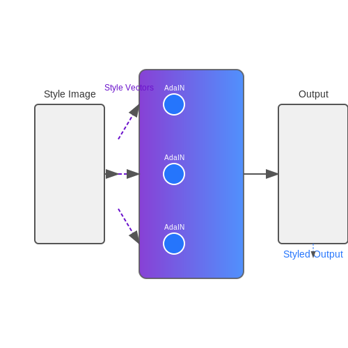
StyleGAN2's disentangled latent space enables seamless integration with neural style transfer techniques, allowing fine-grained control over synthesized content. The key lies in leveraging the style modulation mechanism of StyleGAN2, where style vectors influence feature statistics at different layers. By replacing or interpolating these style vectors with those extracted from a reference style image, we achieve high-fidelity stylization while preserving the underlying structure of the generated image.
Mathematical Formulation
Given a pre-trained StyleGAN2 generator G, let w ∈ W be the intermediate latent code, and s ∈ S be the style vector. The generator applies adaptive instance normalization (AdaIN) at each layer:
where xi is the feature map at layer i, and si contains the scale and shift parameters for that layer. For style transfer, we compute Gram matrices from the reference style image's feature maps and optimize w to minimize the style loss:
where Gi(w) is the Gram matrix of the generated image's features at layer i, and Ĝi is the target Gram matrix from the style image.
Implementation Strategy
To combine StyleGAN2 with style transfer:
- Extract style vectors: Use a pre-trained VGG network to compute feature correlations (Gram matrices) from the style image at multiple scales.
- Latent optimization: Initialize w from the StyleGAN2 latent space and optimize it using gradient descent to minimize both style loss and content preservation loss.
- Layer-wise blending: Apply different style strengths at different resolutions by controlling the weight of style loss terms across StyleGAN2's synthesis network layers.
Practical Considerations
When implementing this approach:
- The truncation trick in StyleGAN2's latent space affects style intensity—lower ψ values produce more conservative stylization.
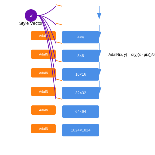
- Coarse layers (4×4 to 8×8) control pose and layout; middle layers (16×16 to 32×32) modify facial features; fine layers (64×64+) handle colors and textures.
- For video stylization, temporal consistency can be enforced by adding optical flow constraints to the optimization.
Advanced Variants
Recent improvements include:
- Conditional Style Transfer: Using CLIP embeddings to guide the stylization process toward text-described styles.
- Patch-based StyleGAN: Applying different styles to different spatial regions by modifying the style vectors per-patch.
- Inversion-based Methods: First inverting the content image to W+ space before style mixing, yielding better structure preservation.
Applications in Image Synthesis and Editing
High-Resolution Image Generation
StyleGAN2's architecture enables the synthesis of high-resolution images (up to 1024×1024 pixels) with fine-grained control over stylistic attributes. The generator employs a progressive growing mechanism, where lower-resolution layers are trained first before gradually introducing higher-resolution layers. This hierarchical approach mitigates artifacts such as texture sticking and phase inconsistencies observed in earlier GANs. The key innovation lies in the adaptive instance normalization (AdaIN) mechanism, which modulates feature statistics at each layer based on a learned style vector w:
Here, xi represents the activations of the i-th layer, while y is the style vector. The modulation ensures that high-level attributes (e.g., pose, lighting) and low-level details (e.g., texture, color) are disentangled.
Latent Space Manipulation
The W-space in StyleGAN2 provides a disentangled latent representation, enabling precise edits to generated images. Linear transformations in W-space correspond to interpretable changes in output images, such as altering facial expressions or adjusting lighting conditions. For example, shifting a latent vector w along a direction Δw learned via supervised methods (e.g., SeFa or InterFaceGAN) yields controlled attribute modifications:
where α controls the strength of the edit. Applications include age progression, gender swapping, and artistic style transfer without retraining the model.
Image Inversion and Editing
Real-image editing requires projecting an input image into StyleGAN2's latent space. Optimization-based methods (e.g., e4e or ReStyle) minimize the perceptual loss between the original and reconstructed image:
Here, VGG denotes a pretrained feature extractor, and wavg is the mean latent vector. Once inverted, semantic edits can be applied using the same latent-space manipulations as synthetic images.
Style Mixing and Cross-Domain Transfer
StyleGAN2 supports style mixing, where coarse styles (resolution ≤ 64×64) control high-level structure, while fine styles (resolution ≥ 128×128) dictate textures. This property is exploited in cross-domain style transfer—e.g., applying artistic styles to photorealistic portraits. The process involves:
- Extracting style codes from a reference image using a pretrained encoder.
- Injecting the codes into the target image's generator layers via AdaIN.
- Blending styles at different resolutions for hybrid outputs.
Ethical and Practical Considerations
While StyleGAN2 enables powerful applications, its misuse risks include deepfakes and identity manipulation. Mitigation strategies involve watermarking synthetic images and developing detection algorithms. Practically, memory constraints (∼12GB GPU for 1024×1024 generation) and training instability remain challenges, addressed partially by StyleGAN3's improvements in temporal coherence and noise robustness.
4. Setting Up StyleGAN2 Training Environment
4.1 Setting Up StyleGAN2 Training Environment
System Requirements
StyleGAN2 demands substantial computational resources due to its high-resolution image synthesis capabilities. Training on custom datasets requires:
- GPU: NVIDIA GPUs with at least 16GB VRAM (e.g., RTX 3090, A100) for resolutions ≥1024×1024
- RAM: 32GB+ system memory for data loading and preprocessing
- Storage: NVMe SSD recommended for fast dataset access (100GB+ free space)
- CUDA: Version 11.1 or later with compatible cuDNN (≥8.0.5)
Software Dependencies
The official NVIDIA implementation relies on Python 3.8+ and PyTorch with specific version constraints:
# Core dependencies
torch==1.9.0+cu111
torchvision==0.10.0+cu111
numpy>=1.19.5
pillow>=8.3.2
tqdm>=4.62.2
Additional requirements for the NVIDIA repository include:
- DNNL: Intel's Deep Neural Network Library for CPU optimizations
- Ninja: Build system for compiling custom CUDA kernels
- OpenCV: For image augmentation pipelines
Environment Configuration
Create an isolated conda environment to manage dependencies:
conda create -n stylegan2 python=3.8
conda activate stylegan2
pip install -r requirements.txt
For CUDA kernel compilation, set these environment variables before building:
export CUDA_HOME=/usr/local/cuda-11.1
export PATH=$$CUDA_HOME/bin:$$PATH
export LD_LIBRARY_PATH=$$CUDA_HOME/lib64:$$LD_LIBRARY_PATH
Dataset Preparation
StyleGAN2 expects datasets in TFRecord format for optimal performance. Convert raw images using the provided dataset tool:
python dataset_tool.py \
  --source=/path/to/raw_images \
  --dest=/path/to/tfrecords/dataset.zip \
  --resolution=1024x1024 \
  --transform=center-crop
Key preprocessing considerations:
- Alignment: Faces require consistent landmark alignment (use dlib or manual cropping)
- Resolution: Must be power-of-two (256×256 to 1024×1024)
- Format: PNG or JPEG with consistent color spaces (sRGB recommended)
Training Configuration
The training script (train.py) accepts several critical hyperparameters:
Configure these via command-line arguments:
python train.py \
  --outdir=./training-runs \
  --cfg=stylegan2 \
  --data=/path/to/dataset.zip \
  --gpus=8 \
  --batch=32 \
  --gamma=10 \
  --mirror=1 \
  --aug=ada \
  --metrics=fid50k_full
Critical parameters include:
- --cfg: Architecture variant (stylegan2, stylegan2-ada)
- --gamma: R1 regularization weight (typically 1-100)
- --aug: Adaptive discriminator augmentation strategy
- --metrics: Evaluation metrics (FID, PPL)
Distributed Training
For multi-GPU setups, use PyTorch's DistributedDataParallel with NCCL backend:
torchrun --nproc_per_node=8 train.py \
  --distributed \
  --batch=32 \
  --kimg=25000
Optimize communication overhead by:
- Setting
--batchas a multiple of GPU count - Using gradient accumulation for small batch sizes
- Enabling mixed precision (
--fp16) on Volta/Turing+ GPUs
Fine-Tuning Pre-trained Models
Fine-tuning pre-trained StyleGAN2 models involves adapting a model trained on a large, general dataset to a specific target domain with limited data. This process leverages transfer learning by preserving the learned hierarchical feature representations while adjusting the generator and discriminator weights to better fit the new data distribution. The key challenge lies in balancing adaptation without catastrophic forgetting of the original model's capabilities.
Mathematical Formulation of Fine-Tuning
The fine-tuning objective modifies the original StyleGAN2 loss function to incorporate domain-specific constraints. Let Loriginal be the standard adversarial loss, and Lnew represent the new domain's loss components. The combined loss becomes:
Where λadv, λpath, and λnew are weighting hyperparameters controlling the contribution of each term. The path length regularization Lpath remains crucial during fine-tuning to maintain stable gradient flow through the network.
Critical Implementation Considerations
Effective fine-tuning requires careful attention to several architectural details:
- Learning rate scheduling: Typically 1-2 orders of magnitude lower than initial training rates (10-5 to 10-4)
- Layer freezing: Early layers often remain frozen to preserve low-level features
- Data augmentation: Must match the original training pipeline's augmentation strategy
- Batch size: Limited by GPU memory but should maintain stable batch statistics
Progressive Fine-Tuning Strategy
A proven approach involves gradually unfreezing network components:
- Start with only the final layers trainable for 10-20% of epochs
- Progressively unfreeze intermediate layers in stages
- Finally allow limited adjustments to early layers if needed
This method prevents drastic overwriting of fundamental feature detectors while allowing sufficient adaptation to the target domain.
Monitoring and Evaluation Metrics
Beyond standard GAN metrics like FID (Fréchet Inception Distance), fine-tuning requires additional validation:
Where positive ΔFID indicates successful domain adaptation. Perceptual similarity metrics should also be tracked to ensure the model retains desirable style characteristics from the original training.
Practical Implementation Example
The following code block demonstrates a typical fine-tuning setup for StyleGAN2 using PyTorch:
# Initialize with pre-trained weights
generator = load_stylegan2(pretrained=True)
discriminator = load_discriminator(pretrained=True)

# Freeze early layers
for layer in generator.synthesis[:8]:
    layer.requires_grad_(False)

# Configure optimizer with lower learning rate
opt_g = torch.optim.Adam(generator.parameters(), lr=1e-5, betas=(0, 0.99))
opt_d = torch.optim.Adam(discriminator.parameters(), lr=4e-5, betas=(0, 0.99))

# Training loop with mixed batches
for real_img in target_dataloader:
    # Generate latent code
    z = torch.randn(batch_size, 512)

    # Generate fake image
    fake_img = generator(z)

    # Compute losses
    loss_d = hinge_loss(discriminator(real_img), discriminator(fake_img.detach()))
    loss_g = -torch.mean(discriminator(fake_img))

    # Update weights
    opt_d.zero_grad()
    loss_d.backward()
    opt_d.step()

    opt_g.zero_grad()
    loss_g.backward()
    opt_g.step()
4.3 Debugging Common Training Issues
Vanishing or Exploding Gradients
StyleGAN2, like other deep generative models, is susceptible to vanishing or exploding gradients, particularly when training on high-resolution images. The issue arises when the gradient norm either shrinks to near-zero or grows exponentially during backpropagation, destabilizing training. The gradient penalty term in StyleGAN2's loss function helps mitigate this:
where λ controls the strength of the gradient penalty, D is the discriminator, and ℙ𝑥̂ represents sampled points along straight lines between real and generated data. If gradients still vanish or explode, consider:
- Reducing the learning rate by a factor of 2–5x.
- Increasing the batch size to stabilize gradient estimates.
- Switching from Adam to RMSprop, which is less prone to gradient explosion.
Mode Collapse in the Generator
Mode collapse occurs when the generator produces limited varieties of samples, often ignoring entire modes of the data distribution. StyleGAN2's progressive growing and path length regularization reduce this risk, but it can still manifest if:
- The discriminator becomes too weak, failing to provide meaningful feedback.
- The latent space 𝒲 is insufficiently diversified during training.
To diagnose mode collapse, monitor the Fréchet Inception Distance (FID) and perceptual path length (PPL) metrics. A sudden drop in FID diversity or erratic PPL values indicates collapsing modes. Solutions include:
- Increasing the discriminator's capacity or adding spectral normalization.
- Applying stronger data augmentation (e.g., ADA—adaptive discriminator augmentation).
- Injecting noise at multiple layers in the generator.
Artifacts in Generated Images
StyleGAN2's architecture reduces common artifacts like phase artifacts and blob-like structures, but new issues may emerge, particularly at high resolutions (1024x1024 and above). Common artifacts include:
- Grid-like patterns: Caused by improper upsampling or aliasing. Enable filtered nonlinearities and use nearest-neighbor upsampling.
- Color banding: Due to insufficient color depth in the generator's output. Switch to 16-bit or 32-bit floating-point precision during training.
- Texture sticking: Occurs when style mixing is underutilized. Increase the probability of style mixing during training.
Training Instability at High Resolutions
Training StyleGAN2 at resolutions beyond 512x512 often introduces instability, manifesting as sudden loss spikes or divergent behavior. Key mitigation strategies include:
- Progressive growing refinement: Start at lower resolutions (e.g., 64x64) and gradually increase, freezing earlier layers.
- Mixed-precision training: Use FP16 for convolutions but FP32 for critical operations like gradient penalty.
- Regularization scheduling: Dynamically adjust the weight of path length regularization based on the current resolution phase.
where t is the current training iteration and Ttransition is the transition duration between resolutions.
Discriminator Overfitting
Unlike traditional GANs, StyleGAN2's discriminator is less prone to overfitting due to its emphasis on style-based features. However, overfitting can still occur when:
- The dataset is small (< 10,000 samples).
- The discriminator's receptive field is too large for early training phases.
Solutions include:
- Applying adaptive data augmentation (ADA) with probability p adjusted dynamically based on the discriminator's overfitting heuristic.
- Using lazy regularization, where gradient penalty and path length regularization are computed less frequently.
Hardware-Specific Issues
StyleGAN2's memory footprint grows quadratically with resolution, leading to GPU memory bottlenecks. Common hardware-related failures include:
- CUDA out-of-memory errors: Reduce batch size or use gradient accumulation.
- NaN losses: Often caused by numerical instability in mixed-precision training. Enable gradient clipping or disable FP16 for certain layers.
- Slow training: Use Tensor Cores (Volta/Ampere GPUs) and enable cudnn.benchmark.
5. Bias and Fairness in Generated Images
5.1 Bias and Fairness in Generated Images
Sources of Bias in StyleGAN2-Generated Images
Bias in StyleGAN2-generated images primarily stems from the training dataset, architectural choices, and latent space properties. The model learns to generate images by capturing statistical patterns in the training data, which often reflect societal biases related to gender, race, age, and other attributes. For instance, if a dataset contains predominantly young, light-skinned faces, StyleGAN2 will generate such faces with higher fidelity and frequency. The latent space interpolation properties further amplify these biases, as certain regions of the space may correspond to underrepresented groups with lower density.
where pdata(x) represents the distribution of the training dataset and preal(x) is the true underlying distribution of real-world images. This mismatch leads to biased generation.
Quantifying Bias in Generated Outputs
Several metrics have been proposed to measure bias in generative models. The Perceptual Path Length (PPL) can be adapted to assess how smoothly attributes transition in latent space, with abrupt changes indicating potential bias. Another approach involves training auxiliary classifiers to detect sensitive attributes (e.g., gender, ethnicity) and computing statistical parity:
where Na=1 is the count of samples with attribute a=1 in the real data, and Na=1gen is the corresponding count in generated samples.
Mitigation Strategies
Several approaches can reduce bias in StyleGAN2 outputs:
- Dataset Balancing: Curating training datasets to ensure proportional representation of demographic groups.
- Latent Space Editing: Identifying and modifying bias directions in the latent space using techniques like SeFa (Closed-Form Factorization of Latent Semantics).
- Adversarial Debiasing: Incorporating a fairness loss term during training to penalize biased generation.
- Conditional Generation: Using auxiliary conditioning variables to explicitly control demographic attributes.
Latent Space Debiasing Formulation
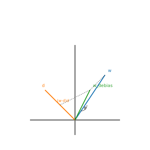
Given a biased latent direction d, we can compute its projection on fairness-sensitive attributes and remove it:
where w is the original latent code and wdebias is the debiased version.
Case Study: Gender Bias in Face Generation
A 2021 study analyzed StyleGAN2 face generation across different ethnicities, finding that generated images of women showed more exaggerated stereotypical features compared to men. The researchers proposed a two-step debiasing approach: first identifying bias directions through linear discriminant analysis in latent space, then applying orthogonal transformations to remove these directions while preserving other semantic features.
Ethical Considerations in Style Transfer
When applying style transfer to human faces, additional ethical concerns arise regarding consent and representation. Transferring artistic styles may inadvertently alter demographic characteristics or create offensive caricatures. Recent work proposes ethical style transfer protocols that include:
- Pre-processing filters to detect and avoid sensitive attributes
- Post-hoc auditing of style-transferred images
- Explicit user controls over attribute preservation
The field continues to develop more sophisticated fairness metrics and debiasing techniques as generative models become more powerful and widely deployed.
5.2 Misuse of Deepfake Technology
Deepfake technology, powered by generative models like StyleGAN2, has enabled highly realistic synthetic media generation. While the underlying mechanisms—such as adversarial training, latent space interpolation, and style transfer—are scientifically fascinating, their misuse poses significant ethical and societal risks. The primary vectors of misuse include disinformation, identity theft, and non-consensual synthetic content.
Technical Foundations of Malicious Deepfakes
At the core of deepfake generation lies the manipulation of latent vectors in StyleGAN2’s W-space or W+-space. Given an input latent code w, the generator G synthesizes an image I = G(w). Adversaries exploit this by optimizing w to minimize a perceptual loss L between the generated image and a target identity:
Here, DLPIPS is the Learned Perceptual Image Patch Similarity metric, and λ terms weight the contributions. Attackers often fine-tune pre-trained models on victim-specific data, leveraging techniques like:
- Few-shot adaptation: Using as few as 10-20 images of the target to personalize the generator.
- Latent space inversion: Projecting real images into W+-space via optimization or encoder networks.
- Voice cloning: Coupling visual deepfakes with synthesized speech using models like Tacotron 2.
Case Studies of High-Impact Misuse
Three documented attack patterns demonstrate the real-world harm potential:
- Political disinformation: In 2022, a deepfake of a European leader declaring false military mobilization caused temporary market instability. The video used StyleGAN2 for facial reenactment and WaveNet for voice synthesis.
- Financial fraud: A 2023 incident involved CEO impersonation via deepfake video conferencing, leading to unauthorized fund transfers. The attack combined face swapping (using FaceShifter) and lip-sync models like Wav2Lip.
- Revenge pornography: Non-consensual intimate imagery (NCII) accounted for 96% of deepfake content in 2021, per Deeptrace Labs. Most cases employed Autoencoder-based face swapping on existing adult content.
Detection and Mitigation Strategies
Current defenses operate at multiple levels:
| Approach | Method | Limitations |
|---|---|---|
| Artifact analysis | Detecting inconsistent eye blinking rates (avg. 0.25 Hz in fakes vs. 0.17 Hz real) | Easily patched by adversarial training |
| Biometric consistency | Heart rate estimation via remote photoplethysmography (rPPG) | Fails with high-quality reenactment |
| Blockchain verification | Provenance tracking with cryptographic hashes | Requires universal adoption |
Emerging solutions include:
where φ represents features from a pretrained Vision Transformer (ViT), and N is the number of sampled latent codes. This measures the divergence between synthetic and natural image manifolds.
Legal and Ethical Countermeasures
Jurisdictions are responding with tailored legislation. The EU’s AI Act (2024) classifies deepfake generation tools as high-risk, requiring:
- Watermarking of all synthetic media
- Documented provenance trails
- Real-time disclosure during consumption
Technical implementations of these requirements face challenges in maintaining robustness against removal attacks while preserving output quality. Current research explores:
- Neural network watermarking via weight perturbation
- Federated learning with differential privacy to limit model leakage
- Adversarial training to resist inversion attacks
5.3 Mitigation Strategies and Best Practices
Addressing Artifacts in StyleGAN2-Generated Images
StyleGAN2, while producing high-fidelity images, is prone to artifacts such as texture sticking, phase artifacts, and inconsistent lighting. These arise due to the progressive growing mechanism and the network's reliance on high-frequency details. A key mitigation strategy involves modifying the generator's architecture to use residual connections and skip connections, which stabilize training and reduce artifacts. The revised architecture minimizes the impact of high-frequency noise by decoupling feature resolution from layer depth.
Here, λ1 and λ2 balance perceptual loss and texture consistency loss, respectively. The perceptual loss ensures global coherence, while the texture loss penalizes local inconsistencies.
Improving Style Transfer Robustness
Style transfer techniques often suffer from content distortion or over-stylization. To mitigate this, adaptive instance normalization (AdaIN) can be replaced with spatially adaptive normalization (SPADE), which preserves structural integrity by conditioning normalization parameters on semantic segmentation maps. This is particularly effective in preserving fine-grained details during transfer.
Key Best Practices:
- Use multi-scale discriminators to evaluate both global and local consistency, reducing mode collapse and artifacts.
- Apply path length regularization to ensure smooth latent space interpolation, avoiding abrupt transitions in generated images.
- Leverage progressive growing with residual blocks to stabilize training and improve output resolution.
Ethical Considerations and Bias Mitigation
StyleGAN2 can amplify biases present in training data, leading to skewed or unethical outputs. Techniques such as dataset balancing, adversarial debiasing, and fairness-aware loss functions are critical. For example, introducing a fairness penalty term in the loss function:
where G(zi) is the generated output and yi is the target distribution. This penalizes deviations from a balanced representation.
Optimizing Training Stability
Training StyleGAN2 requires careful hyperparameter tuning. Key strategies include:
- Learning rate scheduling with warm-up phases to prevent early divergence.
- Gradient penalty to enforce Lipschitz continuity in the discriminator.
- Mixed-precision training to reduce memory overhead while maintaining numerical stability.
Real-World Deployment Considerations
For production systems, model compression techniques such as knowledge distillation or quantization are essential to reduce inference latency. Additionally, deploying a two-stage verification system—where generated images are screened by a lightweight classifier for artifacts—ensures output quality before final delivery.
6. Key Research Papers on StyleGAN2
6.1 Key Research Papers on StyleGAN2
- Image neural style transfer: A review - ScienceDirect — Download: Download high-res image (409KB) Download: Download full-size image Fig. 1. Neural style transfer category. Neural style transfer can be divided into two main categories: style transfer by image iteration (Section 3.1) and style transfer by model iteration (Section 3.2), which use different iteration methods.Image-iteration-based style transfer can be further classified into two ...
- Style Transfer Analysis Based on Generative Adversarial Networks — Style transfer means using a neural network to extract the content of one image and the style of the other image. The two are combined to get the final result, broadly applied in social communication, animation production, entertainment items. Using style transfer, users can share and exchange images; painters can create specific art styles more readily with less creation cost and production ...
- StyleGAN2 Explained - Papers With Code — StyleGAN2 is a generative adversarial network that builds on StyleGAN with several improvements. First, adaptive instance normalization is redesigned and replaced with a normalization technique called weight demodulation. Secondly, an improved training scheme upon progressively growing is introduced, which achieves the same goal - training starts by focusing on low-resolution images and then ...
- Understanding StyleGAN2 - Paperspace Blog — In this article, we go through the StyleGAN2 paper, which is an improvement over StyleGAN1, the key changes are restructuring the adaptive instance normalization using the weight demodulation technique, replacing the progressive growing with the skip connection architecture/residual architecture, and then using the perceptual path length ...
- Styled and characteristic Peking opera facial makeup synthesis with co ... — In this paper, based on deep learning methods, we improve the StyleGAN2 network structure in generative adversarial networks, and propose two models: Co-StyleGAN2 and TC-StyleGAN2, to achieve ...
- Research on GAN-based Text Effects Style Transfer — With the development of neural style transfer and generative adversarial network, the research of text effect style transfer has appeared. The text effect style transfer aims to render text images with style images to produce text effects images. However, for more complex text, the existing methods will generate unrecognizable font images. Therefore, we propose to add morphological methods to ...
- (PDF) Face Generation and Editing with StyleGAN: A Survey - ResearchGate — This inversion was performed using StyleGAN2-ada [4]. Figures - available via license: Creative Commons Attribution-NonCommercial-NoDerivatives 4.0 International Content may be subject to copyright.
- (PDF) Styled and characteristic Peking opera facial makeup synthesis ... — Based on the StyleGAN2 network, we propose a style generative cooperative training network Co-StyleGAN2, which integrates the adaptive data augmentation (ADA) to alleviate the problem of ...
- [2212.09102] Face Generation and Editing with StyleGAN: A Survey - ar5iv — The plan of the paper is as follows: Chapter 1.2 attempts to give an impression of the richness of applications of StyleGAN-based image processing methods. Chapter 2 will explain Generative Adversarial Networks (GANs), delving specifically into the StyleGAN architectures for the generation of face images. Training such architectures needs suitable metrics that capture image similarity at ...
- ToonifyGB: StyleGAN-based Gaussian Blendshapes for 3D Stylized Head Avatars — Figure 1. ToonifyGB: We propose an efficient two-stage framework that employs an improved StyleGAN to generate stylized head videos from input video frames and synthesize the corresponding 3D avatars using Gaussian blendshapes.Our method supports real-time synthesis of stylized avatar animations in styles such as Arcane and Pixar.
6.2 Recommended Books and Tutorials
- Setting up and Running StyleGAN2 - Celantur — Once conda is installed, you can set up a new Python3.6 environment named "stylegan2" with. conda create -n stylegan2 python==3.6.9 # and activates it conda activate stylegan2`. Install GPU-capable TensorFlow and StyleGAN's dependencies: pip install scipy==1.3.3 requests==2.22.0 Pillow==6.2.1 pip install tensorflow-gpu==1.15.3
- PDF Multimodality-guided Image Style Transfer using Cross-modal GAN Inversion — single style transfer, [15] introduced the idea of arbitrary style transfer and aimed to transfer arbitrary styles to any content in a single forward pass. Based on this formula-tion, [6,16,27,29,33,37,42,48] improved [15] on multiple aspects. The above-mentioned methods can be classified as Image-guided Image Style Transfer (IIST). They rely ...
- stylegan2 · GitHub Topics · GitHub — PaddlePaddle GAN library, including lots of interesting applications like First-Order motion transfer, Wav2Lip, picture repair, image editing, photo2cartoon, image style transfer, GPEN, and so on. resolution image-editing gan image-generation pix2pix super-resolution cyclegan edvr stylegan2 motion-transfer first-order-motion-model psgan realsr ...
- Image neural style transfer: A review - ScienceDirect — Download: Download high-res image (409KB) Download: Download full-size image Fig. 1. Neural style transfer category. Neural style transfer can be divided into two main categories: style transfer by image iteration (Section 3.1) and style transfer by model iteration (Section 3.2), which use different iteration methods.Image-iteration-based style transfer can be further classified into two ...
- Style Transfer Analysis Based on Generative Adversarial Networks — Style transfer means using a neural network to extract the content of one image and the style of the other image. The two are combined to get the final result, broadly applied in social communication, animation production, entertainment items. Using style transfer, users can share and exchange images; painters can create specific art styles more readily with less creation cost and production ...
- FACE GENERATION AND EDITING WITH STYLEGAN: A SURVEY - arXiv.org — generated using StyleGAN2 [1]. B. NFT collection [2] gen-erated using StyleGAN2 [1] trained on MetFaces dataset [3]. C. Style mixing (see Figure3). D. From left to right: the source image, smile removed, gender changed [1]. E. Image editing with StyleCLIP [4] using text prompts. Upper row: original images, lower row: edited images using text
- Style Transfer - SpringerLink — As an extension of color transfer, style transfer refers to rendering the content of a target image or video in the style of an artist with either a style sample or a set of images through a style transfer model (Fig. 6.1). As an emerging field, the study of style transfer has attracted the attention of a large number of researchers.
- Style transfer with CycleGAN - DataScientest.com — In this article, we looked at what style transfer is, and more specifically at the architecture of the CycleGAN model, inspired by GANs, for efficient style transfer. CycleGAN is one of the best algorithms for style transfer. We have also seen that this algorithm, unlike almost all style transfer algorithms, does not require matched data, which ...
- PTI: Pivotal Tuning for Latent-based editing of Real Images ... - GitHub — Folder containing models used in different editing techniques and first phase inversion ├ notebooks: Folder with jupyter notebooks to demonstrate the usage of PTI end-to-end ├ scripts: Folder with running scripts for inversion, editing and metric computations ├ torch_utils: Folder containing internal utils for StyleGAN2-ada ├ training
- (PDF) Face Generation and Editing with StyleGAN: A Survey - ResearchGate — of style mixing, b) illustrates how different styles can be used in different levels of the generator (4x4x512), and the latent code z ∈ Z is fed into the network
6.3 Open-Source Implementations and Datasets
- Style Transfer Analysis Based on Generative Adversarial Networks — Style transfer means using a neural network to extract the content of one image and the style of the other image. The two are combined to get the final result, broadly applied in social communication, animation production, entertainment items. Using style transfer, users can share and exchange images; painters can create specific art styles more readily with less creation cost and production ...
- StyleShot: A Snapshot on Any Style - arXiv.org — Our study aims to advance stable and efficient style transfer techniques on the superior image generation capabilities of large diffusion-based T2I models. ... called StyleGallery, covering several open source datasets. Specifically, StyleGallery includes JourneyDB Sun ... we first provide some implementation details about our style-aware ...
- DualStyleGAN - Official PyTorch Implementation - GitHub — The result cartoon_transfer_53_081680.jpg is saved in the folder .\output\, where 53 is the id of the style image in the Cartoon dataset, 081680 is the name of the content face image. An corresponding overview image cartoon_transfer_53_081680_overview.jpg is additionally saved to illustrate the input content image, the encoded content image, the style image (* the style image will be shown ...
- PDF Multimodality-Guided Image Style Transfer Using Cross ... - CVF Open Access — Image Style Transfer (IST) is an interdisciplinary topic of computer vision and art that continuously attracts re-searchers' interests. Different from traditional Image-guided Image Style Transfer (IIST) methods that require a style reference image as input to define the desired style, recent works start to tackle the problem in a text-guided ...
- Awesome Style Transfer Papers - GitHub — A collection of research papers, datasets, and resources related to Style Transfer across various domains. This repository offers a curated list of methods, from traditional techniques to the more recent diffusion models, to provide insights into the ongoing advancements in style transfer.
- stylegan2 · GitHub Topics · GitHub — Open Source Image and Video Restoration Toolbox for Super-resolution, Denoise, Deblurring, etc. Currently, it includes EDSR, RCAN, SRResNet, SRGAN, ESRGAN, EDVR, BasicVSR, SwinIR, ECBSR, etc. ... Official PyTorch Implementation of "GAN-Supervised Dense Visual Alignment" (CVPR 2022 Oral, Best Paper Finalist) ... anime style-transfer stylegan2 ...
- GitHub - temilaj/Style-Transfer-GAN: Demonstrating Neural Style ... — To run the notebook, please clone this repository, start a Jupyter notebook server in the correct directory, and open the notebook called style_transfer_gan.ipynb. This notebook also contains code for a tutorial on how style transfer works; the code for the data in this repo is interspersed throughout.
- Alias-Free Generative Adversarial Networks (StyleGAN3 ... - PythonRepo — Please refer to gen_images.py for complete code example.. Preparing datasets. Datasets are stored as uncompressed ZIP archives containing uncompressed PNG files and a metadata file dataset.json for labels. Custom datasets can be created from a folder containing images; see python dataset_tool.py --help for more information. Alternatively, the folder can also be used directly as a dataset ...
- GRA-GAN: Generative adversarial network for image style transfer of ... — Various datasets that include gender, race, and age information have been widely used recently in studies on face attribute recognition as soft biometrics (Kärkkäinen & Joo, 2019; Liu, Luo, Wang, & Tang, 2015). However, the number of labels in most open datasets is imbalanced, thus being inapplicable to diverse environments.
- What is StyleGAN2 - Activeloop — StyleGAN2 is a powerful generative adversarial network (GAN) that can create highly realistic images by leveraging disentangled latent spaces, enabling efficient image manipulation and editing.