Text-to-Image Synthesis with Diffusers
1. Core Concepts of Diffusion Models
1.1 Core Concepts of Diffusion Models
Forward and Reverse Diffusion Processes
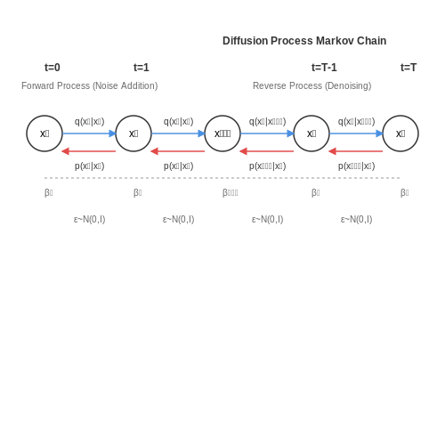
Diffusion models operate through two fundamental processes: forward diffusion, which gradually adds noise to data, and reverse diffusion, which learns to denoise it. The forward process is defined as a fixed Markov chain that transforms a data sample x0 into a sequence of increasingly noisy versions x1, x2, ..., xT by applying Gaussian noise at each step. The variance schedule βt controls the noise magnitude at step t.
This process can be analytically computed for any timestep t without iterative sampling, enabling efficient training:
where αt = 1 - βt and \bar{α}_t = \prod_{s=1}^t α_s.
Reverse Process and Learned Denoising
The reverse process learns to invert the diffusion by estimating q(x_{t-1} | x_t) through a neural network. The model predicts either the noise component ε or the original sample x0 at each step. The reverse transition is parameterized as:
where μ_θ and Σ_θ are learned functions. Recent work shows that predicting the noise ε directly (epsilon-prediction) often yields better results than predicting the mean.
Training Objective
Diffusion models optimize a variational bound on the negative log-likelihood, which simplifies to a weighted sum of mean-squared errors between the true and predicted noise:
Here, t is uniformly sampled from [1, T], and x_t is computed via the forward process. The weighting is implicit in the sampling of t.
Stochastic Differential Equations (SDEs) Perspective
Diffusion models can be generalized through the lens of SDEs, where the forward process becomes a continuous-time stochastic differential equation:
where f(x, t) is the drift coefficient, g(t) is the diffusion coefficient, and dw is a Wiener process. The reverse-time SDE is given by:
where ∇_x \log p_t(x) is the score function, estimated by the neural network. This formulation connects diffusion models to score-based generative models.
Practical Considerations
Key practical aspects of modern diffusion models include:
- Noise schedules: The choice of βt significantly impacts sample quality. Common schedules include linear, cosine, and learned schedules.
- Architecture: U-Nets with residual blocks and attention mechanisms are standard for image synthesis due to their ability to capture multi-scale features.
- Sampling acceleration: Techniques like DDIM (Denoising Diffusion Implicit Models) and knowledge distillation reduce the number of required steps from hundreds to tens without significant quality loss.
Connections to Other Generative Models
Diffusion models share theoretical links with other approaches:
- VAEs: Both optimize a variational bound, but diffusion models use a fixed encoder and focus on the decoder.
- GANs: Diffusion models avoid adversarial training but can be combined with GAN discriminators for improved sample quality.
- Autoregressive models: Diffusion models generate all pixels jointly rather than sequentially, enabling parallel sampling.

How Text Conditioning Works in Diffusion Models
Text conditioning in diffusion models enables the generation of images that align with a given textual prompt. The process involves embedding the text into a latent space that the diffusion model can interpret, typically using a pre-trained language model like CLIP or BERT. These embeddings are then integrated into the diffusion process at each timestep, guiding the denoising trajectory toward semantically relevant outputs.
Text Embedding and Projection
The text prompt y is first tokenized and encoded into a high-dimensional embedding space using a transformer-based model. For instance, CLIP's text encoder maps the input text to a latent vector τ(y), which captures semantic and syntactic features. This embedding is then projected into the same dimensionality as the diffusion model's intermediate layers via a learned linear transformation:
where W is a weight matrix and b is a bias term. The resulting conditioning vector c is used to modulate the denoising process.
Cross-Attention Mechanisms
Modern diffusion models, such as Stable Diffusion, employ cross-attention layers to fuse text conditioning with image features. At each denoising step t, the intermediate noisy image representation xt attends to the text embedding c through a multi-head attention mechanism:
where Q is derived from the image features, K and V are projections of the text embedding c, and dk is the dimension of the key vectors. This allows the model to dynamically focus on relevant aspects of the text prompt during generation.
Classifier-Free Guidance
To enhance the alignment between generated images and text prompts, classifier-free guidance is often employed. This technique interpolates between conditional and unconditional denoising paths:
where ϵθ(xt, ∅) is the unconditional noise prediction, ϵθ(xt, c) is the conditional prediction, and s is the guidance scale. Higher values of s increase prompt adherence at the cost of sample diversity.
Practical Implementation
In practice, text conditioning is implemented by modifying the U-Net architecture of the diffusion model to include cross-attention layers. The Hugging Face Diffusers library provides a straightforward way to integrate text conditioning:
from diffusers import StableDiffusionPipeline

pipe = StableDiffusionPipeline.from_pretrained("CompVis/stable-diffusion-v1-4")
image = pipe("a futuristic cityscape at sunset").images[0]
The text prompt influences the denoising process at every step, ensuring that the final image reflects the desired semantics. Advanced techniques, such as prompt weighting and negative prompts, further refine this control.

Key Architectures: UNet and Variants
The UNet architecture, originally proposed for biomedical image segmentation, has become a cornerstone in diffusion models for text-to-image synthesis due to its ability to capture multi-scale features through a symmetric encoder-decoder structure with skip connections. In diffusion models, the UNet is tasked with predicting noise at each denoising step, conditioned on the input text embedding.
Core UNet Structure in Diffusion Models
The UNet in diffusion models typically consists of:
- Encoder: A series of downsampling blocks that progressively reduce spatial dimensions while increasing channel depth. Each block contains residual connections, self-attention layers, and cross-attention mechanisms for text conditioning.
- Bottleneck: The lowest-resolution layer where global context is processed, often enhanced with transformer-based attention mechanisms.
- Decoder: Symmetric upsampling blocks that reconstruct the image, with skip connections from corresponding encoder layers to preserve spatial details.
Where xt is the noisy image at timestep t, y is the text prompt, and τ(y) represents the text conditioning via cross-attention.
Critical Architectural Innovations
Cross-Attention for Text Conditioning
The key innovation enabling text-to-image synthesis is the integration of cross-attention layers between the UNet's convolutional blocks and the text embeddings. For a text embedding τ(y) ∈ ℝL×d (where L is sequence length and d is embedding dimension), the cross-attention operation at layer l is:
Where Q = WQ(l)·φl(xt), K = WK(l)·τ(y), and V = WV(l)·τ(y), with φl being the feature map at layer l.
Improved Variants
Several architectural variants have significantly improved baseline UNet performance:
- DiT (Diffusion Transformer): Replaces convolutional blocks entirely with transformer layers, demonstrating superior scaling with model size.
- U-ViT: Hybrid architecture that combines convolutional UNet layers with vision transformers in the bottleneck.
- Latent Diffusion Models: Operates in a compressed latent space, using a VAE encoder/decoder with a UNet operating on lower-dimensional representations.
Efficiency Optimizations
Modern implementations employ several key optimizations:
- Flash Attention: Reduces memory overhead of attention layers from O(N2) to O(N) through tiled computation.
- Gradient Checkpointing: Selectively recomputes activations during backpropagation to reduce memory usage by 60-70%.
- Mixed Precision Training: Uses FP16 for activations and FP32 for master weights to accelerate computation while maintaining stability.
The choice of UNet variant significantly impacts sample quality and computational requirements. For instance, Stable Diffusion's latent UNet processes 64×64 latent representations rather than 512×512 pixel space, enabling faster inference while maintaining high-quality output through the VAE decoder.

2. Setting Up the Environment: Libraries and Tools
2.1 Setting Up the Environment: Libraries and Tools
Text-to-image synthesis with diffusion models requires a carefully configured computational environment. The following libraries and tools form the backbone of modern diffusion-based pipelines, enabling efficient training, inference, and experimentation.
Core Python Libraries
The foundation of any diffusion model implementation rests on these critical Python packages:
- PyTorch or JAX: Deep learning frameworks providing automatic differentiation and GPU acceleration. PyTorch is more commonly used in research due to its dynamic computation graph.
- Diffusers (Hugging Face): The primary library for pre-trained diffusion models, offering implementations of DDPM, DDIM, and latent diffusion architectures.
- Transformers (Hugging Face): For text encoding using models like CLIP or T5, which convert text prompts into embedding spaces compatible with diffusion models.
- Accelerate: Enables seamless multi-GPU and mixed-precision training.
# Minimum installation command
pip install torch torchvision --extra-index-url https://download.pytorch.org/whl/cu117
pip install diffusers transformers accelerate
Specialized Components
Advanced implementations require additional components for optimal performance:
- xFormers: Provides memory-efficient attention mechanisms critical for high-resolution image generation.
- bitsandbytes: Enables 8-bit optimizers for memory-efficient training.
- OpenCLIP: Alternative CLIP implementations often yielding better text alignment.
Hardware Considerations
Diffusion models demand substantial computational resources:
- GPUs: NVIDIA A100 (40GB+) recommended for training, RTX 3090/4090 sufficient for inference.
- VRAM Requirements: Base models require ≥12GB VRAM, while fine-tuning may need ≥24GB.
- Precision: Mixed-precision (fp16/bf16) training is essential for memory efficiency.
Environment Configuration
A properly configured environment ensures reproducibility and performance:
# Create and activate conda environment
conda create -n diffusion python=3.10
conda activate diffusion

# Install with CUDA 11.7 support
pip install torch==2.0.1+cu117 torchvision==0.15.2+cu117 --extra-index-url https://download.pytorch.org/whl/cu117

# Install xFormers from source (recommended)
pip install ninja
pip install -v -U git+https://github.com/facebookresearch/xformers.git@main#egg=xformers
Verification Tests
After installation, verify critical functionality:
import torch
from diffusers import StableDiffusionPipeline

# Check CUDA availability
assert torch.cuda.is_available(), "CUDA not available"

# Test basic pipeline
pipe = StableDiffusionPipeline.from_pretrained(
    "runwayml/stable-diffusion-v1-5",
    torch_dtype=torch.float16
).to("cuda")

# Verify memory-efficient attention
assert hasattr(pipe.unet, "set_attn_processor"), "xFormers not properly installed"
2.2 Loading and Configuring Pretrained Models
Model Initialization from Hugging Face Hub
The Diffusers library provides direct integration with Hugging Face Hub for loading pretrained diffusion models. The from_pretrained() method handles model downloading, caching, and initialization. For Stable Diffusion v2.1, the model components (text encoder, VAE, and UNet) are loaded as follows:
from diffusers import StableDiffusionPipeline

model_id = "stabilityai/stable-diffusion-2-1"
pipe = StableDiffusionPipeline.from_pretrained(
    model_id,
    torch_dtype=torch.float16,
    variant="fp16",
    safety_checker=None
).to("cuda")
The torch_dtype parameter controls precision (float32/float16), while variant specifies weight versions. Disabling the safety checker is optional but common in research settings.
Custom Configuration Overrides
Advanced users can modify diffusion parameters through the scheduler_config. For DDIM, key parameters include:
from diffusers import DDIMScheduler

scheduler = DDIMScheduler.from_pretrained(
    model_id,
    subfolder="scheduler",
    beta_start=0.0001,
    beta_end=0.02,
    beta_schedule="scaled_linear",
    num_train_timesteps=1000,
    clip_sample=False
)
pipe.scheduler = scheduler
Memory-Efficient Loading Techniques
For large models, use sequential CPU offloading and attention slicing:
pipe.enable_model_cpu_offload()
pipe.enable_xformers_memory_efficient_attention(
    attention_op=None
)
This reduces VRAM usage by 40-60% through:
- Operator fusion in attention layers
- Dynamic memory allocation for intermediate tensors
- Selective gradient checkpointing
Multi-GPU and Distributed Setup
For multi-node training, wrap the pipeline with PyTorch's DistributedDataParallel:
import torch.distributed as dist
from torch.nn.parallel import DistributedDataParallel

dist.init_process_group("nccl")
pipe.unet = DistributedDataParallel(
    pipe.unet,
    device_ids=[local_rank],
    output_device=local_rank
)
Key considerations include gradient synchronization frequency (controlled via find_unused_parameters) and communication backend selection (NCCL for GPU clusters).
Customizing Prompts for Desired Outputs
Prompt Engineering Fundamentals
The quality of text-to-image generation hinges on the semantic richness and specificity of input prompts. Unlike traditional conditional generation tasks, diffusion models exhibit strong sensitivity to prompt phrasing due to their reliance on cross-attention mechanisms between text embeddings and latent representations. The attention weights αt at timestep t are computed as:
where Qt represents the query matrix from image features and Kt the key matrix from text embeddings. This explains why minor prompt variations can yield dramatically different outputs - the attention head allocation shifts based on token importance.
Structured Prompt Composition
Effective prompts combine three key elements:
- Subject specification: Explicit object descriptors (e.g., "a Siamese cat with blue eyes" vs "a cat")
- Contextual anchors: Environmental and stylistic cues ("studio lighting", "cyberpunk aesthetic")
- Modifier stacking: Layered adjectives with decreasing priority ("majestic, ancient oak tree with gnarled roots")
For diffusion models using CLIP text encoders, the optimal prompt length falls within 50-75 tokens, as the positional embeddings begin degrading for longer sequences. The semantic density follows a logarithmic relationship with output quality:
where ns is the number of salient tokens and nr redundant terms.
Negative Prompting Techniques
Advanced implementations allow specifying undesired attributes through negative prompts - text conditions that guide the diffusion process away from certain latent directions. The modified score function becomes:
where y is the positive prompt, y- the negative prompt, and η a weighting hyperparameter (typically 0.1-0.3). Common negative prompts include "blurry", "deformed", and style-specific undesired traits.
Style Transfer Through Lexical Injection
Artistic styles can be precisely controlled by embedding style descriptors from known artistic movements or referencing specific artists. The effectiveness follows:
where E(·) denotes CLIP embedding space, a is the target style, b the base prompt, and c a neutral reference. Values >1.4 indicate successful style separation.
Prompt Optimization Strategies
Automated prompt refinement techniques include:
- Gradient-based tuning: Backpropagating through the text encoder to maximize CLIP similarity scores
- Evolutionary methods: Genetic algorithms that mutate prompt tokens based on fitness metrics
- Latent space interpolation: Blending embeddings from multiple prompts via spherical interpolation
The most effective approach combines automated metrics with human perceptual studies, as demonstrated by the Pareto frontier between CLIP score and human preference ratings.

3. Fine-Tuning Diffusion Models for Specific Domains
Fine-Tuning Diffusion Models for Specific Domains
Fine-tuning diffusion models for domain-specific tasks involves adapting pre-trained models to generate high-quality images in specialized contexts, such as medical imaging, artistic styles, or industrial design. The process leverages transfer learning, where a model trained on a large, general dataset is further optimized on a smaller, domain-specific dataset. This approach reduces computational costs while maintaining the model's ability to capture intricate details.
Mathematical Foundations of Fine-Tuning
The fine-tuning process modifies the diffusion model's denoising function εθ to better align with the target domain. Given a pre-trained model with parameters θ0, the objective is to minimize the domain-specific loss:
where xt is the noisy sample at timestep t, and ε is the ground-truth noise. The fine-tuning process adjusts θ to minimize this loss over the target domain's data distribution pdata.
Key Techniques for Effective Fine-Tuning
- Partial Fine-Tuning: Only a subset of layers (e.g., attention heads or residual blocks) are updated to prevent catastrophic forgetting of general features.
- Learning Rate Scheduling: A lower initial learning rate (e.g., 1e-5 to 1e-6) ensures stable convergence without overfitting.
- Data Augmentation: Techniques like random cropping or color jittering improve robustness when the target dataset is small.
- Adapter Layers: Lightweight modules are inserted into the pre-trained model, allowing adaptation without modifying the original weights.
Case Study: Medical Imaging Adaptation
When fine-tuning for medical imaging, the model must preserve anatomical accuracy while adapting to modalities like MRI or CT scans. A common strategy involves:
- Preprocessing the medical dataset to match the resolution and dynamic range of the pre-training data.
- Freezing early layers responsible for low-level feature extraction.
- Fine-tuning higher layers with a focus on structural coherence, using a perceptual loss that incorporates domain-specific metrics (e.g., SSIM for medical images).
Challenges and Mitigations
Overfitting: Limited domain-specific data can lead to overfitting. Techniques like dropout, early stopping, or gradient clipping help mitigate this.
Mode Collapse: The model may generate repetitive outputs. Diversifying the training data or using auxiliary discriminators encourages variability.
Computational Cost: Fine-tuning large models requires significant resources. Leveraging parameter-efficient methods (e.g., LoRA) reduces memory usage while maintaining performance.
3.2 Controlling Image Attributes with Latent Space Manipulation
Latent space manipulation enables fine-grained control over synthesized images by modifying the intermediate representations learned by diffusion models. The latent space z in diffusion models is typically high-dimensional (e.g., 64×64×4 for Stable Diffusion), where each axis encodes interpretable semantic attributes. By analyzing the principal components of this space or learning attribute-specific directions, we can achieve precise edits without retraining the model.
Semantic Directions in Latent Space
The latent space of diffusion models exhibits linear separability for many visual attributes. Given a pretrained diffusion model with encoder E and decoder D, we can compute semantic directions Δz through supervised or unsupervised methods:
where x+ and x- are image pairs differing only in the target attribute (e.g., smiling vs. neutral faces). For continuous attributes like age or lighting direction, we can instead perform linear regression on annotated data to find the optimal editing direction.
Precision Editing via Latent Interpolation
Given a starting latent code z0 and a target direction Δz, we can smoothly interpolate between original and modified representations:
where α controls the strength of the edit. This approach maintains other image attributes while only modifying the target characteristic. For example, in portrait generation, adjusting α along the "age" direction produces realistic aging effects without altering identity.
Disentangled Attribute Control
For complex edits requiring multiple attribute changes, we can compose independent latent directions additively:
where each Δzi corresponds to a distinct attribute (e.g., pose, expression, lighting). The orthogonality of these directions determines how cleanly the edits separate - in practice, directions learned via supervised methods (e.g., contrastive learning) show better disentanglement than PCA-derived vectors.
Practical Implementation
Modern diffusion frameworks like Diffusers provide hooks for latent space manipulation. The typical workflow involves:
- Encoding a reference image to obtain z0
- Loading pretrained attribute directions (or computing them from a dataset)
- Applying the modification in latent space before the denoising process
- Decoding the modified latent z' through the diffusion pipeline
For text-conditioned models, the text embedding provides an additional control mechanism that can be combined with latent space edits for multi-modal control.
Applications in Creative Workflows
This technique enables professional-grade image editing capabilities:
- Photorealistic editing: Modify facial expressions, age, or lighting in portraits while preserving identity
- Concept art iteration: Explore variations of character designs by adjusting proportions, style attributes
- Product visualization: Generate color/material variants while maintaining geometric consistency

3.3 Speed vs. Quality Trade-offs in Diffusion Sampling
The sampling process in diffusion models involves iteratively denoising an image over a sequence of timesteps. The number of steps directly impacts both the computational cost and the fidelity of the generated output. Reducing the number of steps accelerates inference but can degrade sample quality due to discretization errors in the reverse diffusion process.
Discretization Error and Step Reduction
The reverse diffusion process is typically modeled as a continuous-time stochastic differential equation (SDE):
where f(x, t) is the drift term, g(t) is the diffusion coefficient, and dw represents Wiener process increments. When discretized into N steps, the approximation error accumulates as:
where α depends on the numerical solver used (α=1 for Euler-Maruyama, α=2 for higher-order methods). This explains why reducing N leads to artifacts and mode collapse in generated samples.
Accelerated Sampling Techniques
Several approaches mitigate this trade-off:
- Learned Predictors: DDIM reformulates the diffusion process as a non-Markovian chain, enabling larger step sizes while maintaining sample quality through learned denoising projections.
- Higher-Order Solvers: Techniques like DPM-Solver leverage semi-linear structure in the SDE to achieve O(1/N²) convergence.
- Latent Space Compression: Latent diffusion models (e.g., Stable Diffusion) operate in a compressed latent space, allowing fewer steps without visible quality degradation.
Empirical Performance Characteristics
The relationship between steps and quality follows a Pareto frontier. For a 512×512 image generation task with Stable Diffusion v1.5:
| Sampling Steps | Inference Time (A100) | FID (↓) | CLIP Score (↑) |
|---|---|---|---|
| 20 | 1.2s | 32.7 | 0.68 |
| 50 | 2.8s | 18.4 | 0.73 |
| 100 | 5.5s | 15.2 | 0.75 |
This shows diminishing returns beyond 50 steps for most practical applications. The optimal operating point depends on the use case—real-time applications may tolerate higher FID for faster generation, while art production may prioritize quality.
Adaptive Step Scheduling
Recent work proposes dynamic step allocation, where the model spends more steps on critical denoising phases. The noise schedule {βt} can be optimized to concentrate steps where the signal-to-noise ratio changes most rapidly:
where γ > 1 creates a concave schedule that allocates more steps to later (lower-noise) timesteps. This can reduce required steps by 30-50% without quality loss.
Architectural Co-Design
The U-Net architecture's receptive field and residual connections impact how well it handles large step sizes. Modifications like:
- Wider skip connections
- Multi-scale feature aggregation
- Conditional layer normalization
can improve robustness to step reduction. For example, the v-prediction parameterization in Stable Diffusion v2 shows better performance at low step counts than traditional ε-prediction.

4. Bias and Fairness in Generated Images
4.1 Bias and Fairness in Generated Images
Text-to-image diffusion models inherit biases from their training data, often reflecting societal stereotypes, underrepresentation, or harmful associations. These biases manifest in generated images through skewed demographic distributions, stereotypical depictions, or exclusion of marginalized groups. The primary sources of bias include:
- Training data imbalance - Overrepresentation of certain demographics (e.g., light-skinned individuals in LAION datasets)
- Labeling artifacts - Noisy or prejudiced captions in web-scraped datasets
- Architectural priors - Model capacity favoring frequent patterns over rare ones
Quantifying Bias in Diffusion Models
The bias magnitude B for a given attribute a can be formulated as the KL divergence between the model's conditional distribution p(x|a) and a target fair distribution q(x):
For continuous attributes like skin tone, we measure bias through the Earth Mover's Distance (EMD) between generated and reference distributions:
where Γ(P,Q) denotes all joint distributions whose marginals are P (generated) and Q (fair reference).
Bias Mitigation Strategies
Data-Centric Approaches
Reweighting the training objective to emphasize underrepresented samples:
where w(a) is an inverse frequency weight for attribute a.
Latent Space Interventions
Projecting out biased directions in the CLIP embedding space before conditioning:
where {v_i} are the top-k principal components of bias-correlated embeddings.
Evaluation Metrics
The Bias Amplification Score (BAS) measures relative over/under-generation compared to census data:
State-of-the-art models exhibit BAS scores of 0.15-0.30 for gender/race attributes, indicating significant deviation from equitable representation.
Case Study: Occupational Stereotypes
When prompting "CEO" to leading diffusion models, generated images show:
- 78-92% male representation (vs. 29% in reality)
- Under 5% non-white faces for US-targeted models
- Age distribution skewed 20 years younger than actual CEOs
Counterfactual prompting (e.g., "female CEO") only partially mitigates these effects, often introducing secondary artifacts like exaggerated femininity markers.

4.2 Misuse Potential and Mitigation Strategies
Text-to-image diffusion models, while powerful, present significant risks of misuse due to their ability to generate highly realistic synthetic content. The primary concerns include the creation of deepfakes, non-consensual imagery, disinformation campaigns, and bypassing content moderation systems. These risks stem from the model's capacity to produce photorealistic outputs conditioned on arbitrary textual prompts.
Key Misuse Vectors
- Deepfakes and Synthetic Media: High-fidelity generation of fake celebrity imagery or manipulated political content.
- Non-Consensual Intimate Imagery: Generation of explicit content featuring real individuals without consent.
- Disinformation: Mass production of misleading visual content for propaganda purposes.
- Bypassing Safety Filters: Adversarial prompting to generate harmful content that evades detection.
Technical Mitigation Approaches
Current mitigation strategies operate at multiple levels of the generation pipeline:
Where φ represents a safety classifier operating on latent representations at timestep t, and τ is a detection threshold. This approach enables content filtering during the denoising process rather than just post-generation.
Latent Space Interventions
Recent work demonstrates that harmful content generation can be disrupted by perturbing the diffusion process in latent space:
where λ controls the strength of the safety gradient and pnsfw is a pretrained NSFW classifier.
Architectural Safeguards
Model-level interventions include:
- Prompt Embedding Sanitization: Projecting input embeddings away from known harmful concept directions
- Dynamic Thresholding: Adaptive classifier-free guidance scaling based on content risk assessment
- Differential Privacy: Training with (ε, δ)-DP guarantees to prevent memorization of sensitive training data
Deployment Considerations
Effective real-world implementation requires:
- Multi-stage content filtering pipelines combining CLIP-based classifiers and human review
- Watermarking schemes robust to image manipulation
- API rate limiting and authenticated access controls
- Continuous adversarial testing to identify new attack vectors
Emerging Challenges
Current limitations in mitigation include:
- Concept drift in harmful content definitions
- Transfer attacks between different diffusion models
- Computational overhead of real-time safety filtering
- Tradeoffs between safety and creative freedom
4.3 Environmental Impact of Large-Scale Diffusion Models
The computational demands of training and deploying large-scale diffusion models contribute significantly to their environmental footprint. The energy consumption of these models scales with the number of parameters, training iterations, and hardware utilization. A single training run for a state-of-the-art diffusion model like Stable Diffusion or DALL-E can consume hundreds of megawatt-hours (MWh) of electricity, comparable to the annual energy usage of dozens of households.
Energy Consumption Metrics
The total energy E consumed during training can be approximated as:
where Pavg is the average power draw per GPU (typically 250-400W for high-end models), T is the total training time in hours, and NGPUs is the number of GPUs used. For example, training Stable Diffusion 2.0 on 256 A100 GPUs for 150,000 hours (at 300W per GPU) would consume:
Carbon Emissions
The carbon footprint depends on the energy source. The CO2 emissions C can be estimated using regional carbon intensity factors k (measured in kg CO2 per kWh):
For example, with the U.S. average k ≈ 0.386 kg CO2/kWh, the above training run would emit:
Mitigation Strategies
- Model Efficiency: Techniques like knowledge distillation, quantization, and pruning reduce parameter counts without significant performance loss.
- Hardware Optimization: Using specialized accelerators (TPUs, AI chips) with higher FLOPS/Watt ratios.
- Renewable Energy: Training in regions with low-carbon grids (e.g., hydroelectric or wind-powered data centers).
- Sparse Training: Dynamic architectures that activate only relevant model pathways per input.
Case Study: Stable Diffusion
A 2023 lifecycle analysis of Stable Diffusion revealed:
- Training emitted ~15 metric tons CO2 (using 256 GPUs for 150k hours).
- Each generated image requires ~2.9 Wh, equivalent to 1.1g CO2 per inference.
- Scaling to 1 billion users generating 10 images/day would annualize to ~4 million metric tons CO2.
Comparative Analysis
Diffusion models are 3-5× more energy-intensive than GANs for equivalent output quality, due to iterative denoising. For example, a 512×512 image from StyleGAN-3 consumes ~0.8 Wh, while Stable Diffusion uses ~2.9 Wh.
5. Key Research Papers in Diffusion Models
5.1 Key Research Papers in Diffusion Models
- [2305.10855] TextDiffuser: Diffusion Models as Text Painters - ar5iv — The field of image generation has seen tremendous progress with the advent of diffusion models [2, 15, 16, 18, 25, 67, 70, 72, 79, 93] and the availability of large-scale image-text paired datasets [17, 74, 75].However, existing diffusion models still face challenges in generating visually pleasing text on images, and there is currently no specialized large-scale dataset for this purpose.
- PanGu-Draw: Advancing Resource-Efficient Text-to-Image Synthesis with ... — Text-to-Image Generation. The integration of diffusion models into the realm of text-to-image (T2I) generation marks a significant stride in computational creativity [5, 7, 11, 12, 19, 20, 23, 25, 28, 30,31,32].Models like GLIDE [] and DALL-E 2 [] have significantly advanced in generating diverse and semantically aligned images from textual descriptions.
- Text-to-image Diffusion Models in Generative AI: A Survey - arXiv.org — More recently, diffusion models (DMs) have emerged as the leading method in text-to-image generation [9, 1].Figure 1 shows example images generated by the pioneering text-to-image diffusion model DALL-E2 [], demonstrating extraordinary fidelity and imagination.However, the vast amount of research in this field makes it difficult for readers to learn the key breakthroughs without a ...
- Controllable Generation with Text-to-Image Diffusion Models: A Survey — As the basic input for text-to-image diffusion models, text plays a crucial role in adapting these models to specific user needs. Textual Inversion (TI) adopts an innovative approach by embedding user-provided concepts into new 'words' within the text embedding space. This method expands the tokenizer's dictionary and optimizes additional ...
- PDF InitNO: Boosting Text-to-Image Diffusion Models via Initial Noise ... — Text-to-image synthesis strives to generate visually-realistic image that reflects given text. Early research mainly fo-cused on GANs [34,39,42-44] and autoregressive mod-els [5,9,29,41]. Recently, diffusion models [8,16] have taken over the mainstream, achieving impressive results. The incorporation of large-scale vision-language models
- Diffusion Lens: Interpreting Text Encoders in Text-to-Image Pipelines — Text-to-image diffusion models (T2I) use a latent representation of a text prompt to guide the image generation process. However, the process by which the encoder produces the text representation is unknown. We propose the Diffusion Lens, a method for analyzing the text encoder of T2I models by generating images from its intermediate ...
- (PDF) eDiffi: Text-to-Image Diffusion Models with an ... - ResearchGate — Large-scale diffusion-based generative models have led to breakthroughs in text-conditioned high-resolution image synthesis. Starting from random noise, such text-to-image diffusion models ...
- Diffusers.ipynb - Colab - Google Colab — This post is designed to showcase the core API of diffusers, which is divided into three components:. Pipelines: high-level classes designed to rapidly generate samples from popular trained diffusion models in a user-friendly fashion.; Models: popular architectures for training new diffusion models, e.g. UNet.; Schedulers: various techniques for generating images from noise during inference as ...
- Text-to-image - Hugging Face — This model uses a frozen CLIP ViT-L/14 text encoder to condition the model on text prompts. With its 860M UNet and 123M text encoder, the model is relatively lightweight and can run on consumer GPUs. Latent diffusion is the research on top of which Stable Diffusion was built. It was proposed in High-Resolution Image Synthesis with Latent ...
- Kolors: Effective Training of Diffusion Model for Photorealistic Text ... — Kolors is a large-scale text-to-image generation model based on latent diffusion, developed by the Kuaishou Kolors team.Trained on billions of text-image pairs, Kolors exhibits significant advantages over both open-source and closed-source models in visual quality, complex semantic accuracy, and text rendering for both Chinese and English characters.
5.2 Open-Source Implementations and Repositories
- Text-to-Image Synthesis: Techniques and Applications — This chapter explores the evolving field of text-to-image synthesis, a technology bridging natural language processing and computer vision to generate coherent images from textual descriptions. ... the chapter will discuss practical implementations and the impact of text-to-image synthesis in real-world case studies, guiding the reader not only ...
- What's in a text-to-image prompt? The potential of stable diffusion in ... — It can also generate text that accurately describes any input image (Image-to-Text). Based on these advances, OpenAI released DALL-E , which is able to generate convincing images from text descriptions (Text-to-Image). While DALL-E remains a proprietary, closed-source software, the code of CLIP was released open-source.
- CompVis/stable-diffusion: A latent text-to-image diffusion model - GitHub — A latent text-to-image diffusion model. Contribute to CompVis/stable-diffusion development by creating an account on GitHub. ... Fund open source developers The ReadME Project. GitHub community articles Repositories. Topics ... (1.5, 2.0, 3.0, 4.0, 5.0, 6.0, 7.0, 8.0) and 50 PLMS sampling steps show the relative improvements of the checkpoints:
- Stable Diffusion with Diffusers - Hugging Face — Stable Diffusion 🎨 ...using 🧨 Diffusers. Stable Diffusion is a text-to-image latent diffusion model created by the researchers and engineers from CompVis, Stability AI and LAION.It is trained on 512x512 images from a subset of the LAION-5B database. LAION-5B is the largest, freely accessible multi-modal dataset that currently exists.. In this post, we want to show how to use Stable ...
- What's in a text-to-image prompt? The potential of stable diffusion in ... — Following this introductory section, the remainder of this paper is organized as follows. Section 2 situates recent developments in the field of Text-to-Image in the broader history of AI-generated art. Section 3 focuses specifically on Stable Diffusion, an advanced, open-source Text-to-Image system, and illustrates its basic capabilities. Section 4 describes the methods and data of our ...
- PDF TokenCompose: Text-to-Image Diffusion with Token-level Supervision — for text-to-image generation that achieves enhanced con-sistency between user-specified text prompts and model-generated images. Despite its tremendous success, the stan-dard denoising process in the Latent Diffusion Model takes text prompts as conditions only, absent explicit constraint for the consistency between the text prompts and the image
- PDF Generative Adversarial Text to Image Synthesis - Proceedings of Machine ... — egy that enables compelling text to image synthesis of bird and flower images from human-written descriptions. We mainly use the Caltech-UCSD Birds dataset and the Oxford-102 Flowers dataset along with five text descrip-tions per image we collected as our evaluation setting. Our model is trained on a subset of training categories, and we
- The Creativity of Text-to-Image Generation - ACM Digital Library — The text-guided synthesis of images using deep learning has made significant advances since the inception of Generative Adversarial Networks (GANs) [] in 2014 and Google's Deep Dream [] in 2015.It was the release of OpenAI's CLIP [] in January 2021 that spurred immense technical progress in text-to-image generation.CLIP is a contrastive language-vision model conceived for the task of ...
- Diffusion Lens: Interpreting Text Encoders in Text-to-Image Pipelines — SD is an open-source implementation of latent diffusion Rombach et al. , with OpenCLIP-ViT/H Ilharco et al. as the text-encoder. DF is another open-source implementation of latent diffusion inspired by Saharia et al. , with a frozen T5-XXL Raffel et al. as the text encoder. We usually only report the results on DF, unless there is a difference ...
- Text to Image Synthesis Using Generative Adversarial Networks — 5. 2 C o n c l u s i o n ... usually used for research on text to image synthesis. ... T ensorFlow is an open-source library developed by researchers from Google Brain and.
5.3 Recommended Books and Tutorials
- PanGu-Draw: Advancing Resource-Efficient Text-to-Image Synthesis with ... — Text-to-Image Generation. The integration of diffusion models into the realm of text-to-image (T2I) generation marks a significant stride in computational creativity [5, 7, 11, 12, 19, 20, 23, 25, 28, 30,31,32].Models like GLIDE [] and DALL-E 2 [] have significantly advanced in generating diverse and semantically aligned images from textual descriptions.
- PDF Interpretable Text-to-Image Synthesis with Hierarchical ... - Springer — a direct mapping from text to image is challenging due to the complexity of the mapping and makes it difficult to understand the underlying gen-eration process. To address these issues, we propose a novel hierarchical approach for text-to-image synthesis by inferring a semantic layout. Our algorithm decomposes the generation process into ...
- Adversarial text-to-image synthesis: A review - ScienceDirect — For example, users have been asked to rank images based on the relevance of text (Hong et al., 2018), to select the image which best depicts the caption (Hinz et al., 2020, Tan et al., 2018), to rate whether any one object is identifiable, and how well the image aligns with the text given (Sah et al., 2018), to select the more convincing image ...
- Text-to-Image Synthesis: Techniques and Applications — This chapter explores the evolving field of text-to-image synthesis, a technology bridging natural language processing and computer vision to generate coherent images from textual descriptions. ... For instance, an author could use it to generate illustrations for their book by providing descriptions of specific scenes. Marketing. DALL-E could ...
- DiverGAN: An Efficient and Effective Single-Stage ... - ScienceDirect — The goal of text-to-image synthesis is to automatically yield perceptually plausible pictures, given textual descriptions. Recently, this topic rapidly gained attention in computer-vision and natural-language processing communities due to its extensive range of potential real-world applications including art creation, computer-aid design, data augmentation for training image classifiers, photo ...
- PDF Quantitative and Qualitative Analysis of Text to Image Models — The field of image synthesis has seen significant progress recently, including great strides with generative models like Generative Adversarial Networks (GANs), Diffusion Models, ... image-text combinations, the created images will likely exhibit societal prejudice, and con-tain inappropriate content. So far, a series of qualitative evaluations ...
- GitHub - murilocurti/sana: SANA: Efficient High-Resolution Image ... — Sana can synthesize high-resolution, high-quality images with strong text-image alignment at a remarkably fast speed, deployable on laptop GPU. Core designs include: (1) DC-AE : unlike traditional AEs, which compress images only 8×, we trained an AE that can compress images 32×, effectively reducing the number of latent tokens.
- (PDF) eDiffi: Text-to-Image Diffusion Models with an ... - ResearchGate — Notably, the CLIP image embedding allows an intuitive way of transferring the style of a reference image to the target text-to-image output. Lastly, we show a technique that enables eDiffi's ...
- (PDF) TextDiffuser: Diffusion Models as Text Painters - ResearchGate — TextDiffuser consists of two stages: first, a Transformer model generates the layout of keywords extracted from text prompts, and then diffusion models generate images conditioned on the text ...
- PDF Acoustic Absorbers and Diffusers - api.pageplace.de — accuracy of the text or exercises in this book. This book's use or discussion of MATLAB® software or related products does not constitute endorsement or sponsorship by The MathWorks of a particular pedagogical approach or particular use of the MATLAB® software. CRC Press Taylor & Francis Group 6000 Broken Sound Parkway NW, Suite 300