

Variational Autoencoders (VAEs)
1. Key Concepts: Latent Variables and Probabilistic Modeling
Key Concepts: Latent Variables and Probabilistic Modeling
Latent Variables in Generative Models
Latent variables are unobserved random variables that capture the underlying structure of observed data. In generative modeling, they serve as a compressed representation of the data, enabling efficient sampling and inference. For a dataset X with observations x1, ..., xN, the latent variables z1, ..., zN are drawn from a prior distribution p(z), typically chosen as a standard Gaussian:
The joint distribution of observed and latent variables is p(x, z) = p(x|z)p(z), where p(x|z) is the likelihood function. The goal is to learn the true posterior p(z|x), which is often intractable for complex models.
Probabilistic Modeling and Approximate Inference
Variational Autoencoders (VAEs) address intractability by introducing an approximate posterior qϕ(z|x), parameterized by a neural network with weights ϕ. This distribution is optimized to minimize the Kullback-Leibler (KL) divergence between qϕ(z|x) and the true posterior p(z|x):
Minimizing this divergence is equivalent to maximizing the Evidence Lower Bound (ELBO):
where θ parameterizes the generative model pθ(x|z). The first term is the reconstruction loss, while the second term regularizes the approximate posterior to remain close to the prior.
Reparameterization Trick
To enable gradient-based optimization, VAEs employ the reparameterization trick. Instead of sampling z directly from qϕ(z|x), we express z as a deterministic function of a noise variable ϵ ∼ p(ϵ):
Here, μϕ(x) and σϕ(x) are outputs of the encoder network, and ⊙ denotes element-wise multiplication. This allows backpropagation through stochastic layers.
Practical Implications
VAEs are widely used for tasks like image generation, anomaly detection, and semi-supervised learning. Their probabilistic nature enables uncertainty quantification, while the latent space allows for meaningful interpolations and controlled generation. For example, in medical imaging, VAEs can model variations in anatomical structures while preserving key diagnostic features.

Autoencoders vs. VAEs: Core Differences
Traditional autoencoders and variational autoencoders (VAEs) share an encoder-decoder architecture but diverge fundamentally in their objectives, mathematical foundations, and generative capabilities. The key distinction lies in how they handle latent space representations and the probabilistic nature of VAEs.
Deterministic vs. Probabilistic Latent Space
Autoencoders learn a deterministic mapping from input space x to latent space z through the encoder function z = f(x). The decoder then reconstructs the input as x̂ = g(z). This approach minimizes reconstruction loss (typically mean squared error) without imposing any constraints on the organization of the latent space.
VAEs instead model the latent space as a probability distribution. The encoder outputs parameters (μ, σ) of a Gaussian distribution, and latent vectors are sampled via the reparameterization trick:
The Kullback-Leibler Divergence Term
VAEs introduce a critical regularization term that forces the learned latent distribution q(z|x) to approximate a prior p(z) (typically standard normal). The VAE loss combines reconstruction error with KL divergence:
Where β controls the trade-off between reconstruction quality and latent space regularization. This explicit probabilistic formulation enables two capabilities absent in standard autoencoders:
- Controlled generation: Sampling from p(z) yields meaningful outputs
- Latent space interpolation: Points between encoded samples remain semantically meaningful
Architectural Implications
The probabilistic approach necessitates specific architectural choices:
- The encoder outputs two vectors (μ and log σ²) instead of a single latent code
- The decoder receives stochastic inputs during training but deterministic inputs during inference
- Bottleneck width becomes less critical as the model learns distributed representations
Practical Performance Characteristics
In practice, VAEs exhibit different behaviors from autoencoders:
| Property | Autoencoder | VAE |
|---|---|---|
| Reconstruction fidelity | Higher | Lower (trade-off for generation) |
| Training stability | More stable | Requires careful β tuning |
| Latent space organization | Arbitrary | Gaussian, continuous |
The choice between architectures depends on the application: autoencoders excel at compression and anomaly detection, while VAEs are preferred for generative tasks and latent space manipulation.

The Role of the Variational Lower Bound (ELBO)
The variational lower bound, or Evidence Lower Bound (ELBO), is central to the training of Variational Autoencoders (VAEs). It serves as a surrogate objective function that allows efficient optimization of the intractable marginal log-likelihood. The ELBO is derived from the Kullback-Leibler (KL) divergence between the approximate posterior q(z|x) and the true posterior p(z|x):
By rearranging the KL divergence, we obtain the ELBO as a lower bound on the log-likelihood of the data:
The first term, 𝔼q(z|x)[log p(x|z)], represents the reconstruction loss, encouraging the decoder to generate samples that match the input data. The second term, DKL(q(z|x) ∥ p(z)), acts as a regularizer, ensuring the learned posterior q(z|x) stays close to the prior p(z), typically a standard Gaussian.
Decomposition of the ELBO
The ELBO can be decomposed into two interpretable components:
- Reconstruction Term: Measures how well the generated samples match the input data, akin to an autoencoder’s reconstruction error.
- KL Divergence Term: Penalizes deviations of the learned latent distribution from the prior, promoting a well-structured latent space.
This decomposition highlights the trade-off between accurate reconstruction and latent space regularization, which is crucial for avoiding overfitting and ensuring meaningful latent representations.
Optimization and Practical Implications
Maximizing the ELBO is equivalent to minimizing the KL divergence between the approximate and true posteriors. However, direct computation of the expectation term is often intractable. Instead, VAEs employ the reparameterization trick, enabling gradient-based optimization through stochastic sampling:
This allows backpropagation through the sampling process, making training feasible. In practice, the ELBO is estimated using Monte Carlo sampling:
where L is the number of samples, often set to L=1 for computational efficiency.
Connection to Variational Inference
The ELBO is not unique to VAEs—it originates from variational inference, where the goal is to approximate complex posterior distributions. In VAEs, the encoder q(z|x) acts as the variational distribution, and the ELBO provides a tractable objective for learning both the encoder and decoder parameters.
This formulation bridges probabilistic modeling and deep learning, enabling VAEs to generate diverse and high-quality samples while maintaining a principled probabilistic framework.
2. Probabilistic Graphical Models for VAEs
2.1 Probabilistic Graphical Models for VAEs
Variational Autoencoders (VAEs) are fundamentally grounded in probabilistic graphical models (PGMs), which provide a structured framework for representing dependencies between random variables. The core PGM for VAEs consists of observed variables x (data) and latent variables z, with directed edges encoding conditional dependencies. The joint distribution factorizes as:
Here, p(z) is the prior over latent variables, typically chosen as a standard Gaussian N(0, I), while p(x|z) is the generative model (decoder) that maps latent variables to observed data. The true posterior p(z|x) is intractable for complex models, necessitating variational inference with an approximate posterior q(z|x) (encoder).
Directed Acyclic Graph Representation
The PGM for a VAE is a directed acyclic graph (DAG) with the following structure:
- Latent variables z are root nodes sampled from the prior p(z).
- Observed variables x are leaf nodes conditioned on z via p(x|z).
- The variational posterior q(z|x) introduces an inverse dependency (dashed edge) for inference.
This structure reflects the generative process: latent variables z generate observations x, while the encoder q(z|x) approximates the reverse mapping for inference.
Evidence Lower Bound (ELBO) Derivation
The learning objective for VAEs is derived by maximizing the ELBO, which bounds the log-likelihood of the data:
The first term is the reconstruction loss, encouraging the decoder to generate accurate outputs. The second term is the Kullback-Leibler (KL) divergence between the approximate posterior and prior, acting as a regularizer to keep q(z|x) close to p(z).
Conditional Independence Assumptions
VAEs leverage conditional independence assumptions to simplify inference:
- Factorized prior: p(z) = \prod_i p(z_i) (typically isotropic Gaussian).
- Factorized approximate posterior: q(z|x) = \prod_i q(z_i|x) (mean-field assumption).
- Decoder independence: p(x|z) = \prod_j p(x_j|z) for data dimensions.
These assumptions enable efficient computation and scalability to high-dimensional data.
Extensions with Structured PGMs
Advanced VAEs extend the basic PGM to capture richer dependencies:
- Hierarchical VAEs: Introduce multiple layers of latent variables z_1, z_2, ..., z_L with hierarchical dependencies.
- Graphical VAEs: Replace mean-field assumptions with structured q(z|x) using autoregressive or flow-based models.
- Conditional VAEs: Incorporate observed context c via p(x|z, c) and q(z|x, c).
These extensions demonstrate the flexibility of PGMs in designing VAEs for complex data distributions.

2.2 The Reparameterization Trick
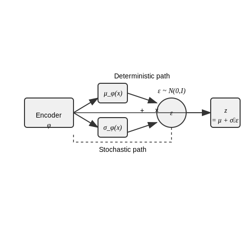
The reparameterization trick is a critical technique for enabling gradient-based optimization in variational autoencoders (VAEs). It addresses a fundamental challenge: sampling from the latent space distribution z ~ qφ(z|x) introduces stochasticity that breaks differentiability, preventing backpropagation through the sampling operation.
Mathematical Motivation
In VAEs, the latent variable z is typically sampled from a Gaussian distribution parameterized by the encoder:
Directly sampling z this way makes the gradient ∇φ with respect to the encoder parameters φ undefined. The reparameterization trick circumvents this by expressing z as a deterministic function of φ and an auxiliary noise variable ε:
This reformulation separates the stochastic part (ε) from the differentiable parameters (μφ, σφ), allowing gradients to flow through the deterministic path during backpropagation.
Derivation and Properties
The trick works because any sample from N(μ, σ²) can be rewritten as μ + σε, where ε ~ N(0,1). This preserves the original distribution's properties while making the sampling process differentiable:
The gradient of the expectation can now be computed as:
Practical Implementation
In practice, the reparameterization trick is implemented by:
- Computing μφ(x) and σφ(x) via the encoder network
- Sampling ε from a standard normal distribution
- Calculating z = μφ(x) + σφ(x) ⊙ ε
This approach is not limited to Gaussian distributions. For other continuous distributions (e.g., exponential, logistic), similar reparameterizations exist where the random variable can be expressed as a differentiable transformation of a fixed base distribution.
Impact on Training Stability
The reparameterization trick significantly improves VAE training by:
- Reducing variance in gradient estimates compared to score function estimators
- Enabling efficient computation of low-variance gradients
- Allowing the use of standard backpropagation through the entire architecture
This technique is why modern VAEs can effectively optimize the evidence lower bound (ELBO) and learn meaningful latent representations.
KL Divergence and Its Importance in VAEs
The Kullback-Leibler (KL) divergence serves as a fundamental component in variational autoencoders, quantifying the difference between the approximate posterior distribution qφ(z|x) and the prior distribution p(z) over latent variables. This non-symmetric measure, defined as:
acts as a regularization term in the VAE objective function, preventing the encoder from deviating too far from the prior while maintaining meaningful latent representations. For the common choice of a standard Gaussian prior p(z) = 𝒩(0, I) and diagonal Gaussian posterior qφ(z|x) = 𝒩(μφ(x), σφ(x)), the KL term admits a closed-form solution:
where J represents the dimensionality of the latent space. This analytical form enables efficient computation during training through backpropagation.
Role in the VAE Loss Function
The total VAE loss combines the reconstruction error (negative log-likelihood) with the KL divergence term:
This formulation reveals the KL divergence's dual function: it regularizes the latent space while enabling the probabilistic interpretation of the model. The β-VAE extension introduces a tunable parameter to control the strength of this regularization:
Geometric Interpretation
From an information geometry perspective, the KL divergence induces a Riemannian metric on the manifold of probability distributions. In VAEs, this manifests as:
- Manifold learning: The KL term encourages the latent space to maintain topological properties similar to the prior
- Representation control: It prevents posterior collapse where latent dimensions become uninformative
- Capacity tuning: The divergence automatically adjusts the effective dimensionality of the latent space
Practical Considerations
Several advanced techniques address challenges with the KL term in practice:
- KL annealing: Gradually increasing the weight of the KL term during training prevents initial suppression of latent variables
- Free bits: Implementing a minimum KL per dimension ensures no latent feature gets completely pruned
- Alternative divergences: The χ2-divergence or Wasserstein distance sometimes offer improved properties
Recent work on disentangled representations shows that careful manipulation of the KL term, particularly through controlled increases in β, can lead to more interpretable latent spaces where individual dimensions correspond to semantically meaningful factors of variation.
3. Encoder and Decoder Networks
Encoder and Decoder Networks
The encoder and decoder networks in a Variational Autoencoder (VAE) form the backbone of its architecture, enabling the transformation of high-dimensional input data into a lower-dimensional latent space and back. Unlike traditional autoencoders, VAEs impose a probabilistic structure on the latent space, allowing for generative capabilities.
Encoder Network
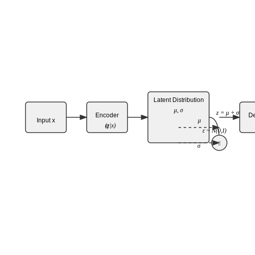
The encoder, denoted as qϕ(z|x), maps input data x to a latent variable z by approximating the posterior distribution. It is typically implemented as a neural network with parameters ϕ. For a Gaussian latent space, the encoder outputs the mean μ and log-variance log σ2 of the distribution:
Here, μ_ϕ(x) and σ_ϕ(x) are learned functions of the input. The use of log-variance ensures numerical stability during training. The reparameterization trick is employed to enable gradient-based optimization:
where ⊙ denotes element-wise multiplication. This trick allows backpropagation through stochastic sampling.
Decoder Network
The decoder, denoted as pθ(x|z), reconstructs the input data from the latent variable z. It is another neural network with parameters θ, modeling the likelihood of the data given the latent representation. For continuous data, the decoder often outputs the parameters of a Gaussian distribution:
For binary data, a Bernoulli distribution is more appropriate:
where D is the dimensionality of the input data.
Architecture Choices
Both the encoder and decoder are typically implemented as multi-layer perceptrons (MLPs) or convolutional neural networks (CNNs), depending on the data type:
- MLPs are suitable for tabular or flattened data.
- CNNs are preferred for image data, leveraging spatial hierarchies.
- Recurrent architectures (e.g., LSTMs) may be used for sequential data.
The choice of activation functions is critical. The encoder often uses ReLU or LeakyReLU for hidden layers, while the output layer for μ is linear and for log σ2 is also linear or clamped. The decoder's output activation depends on the data type:
- Sigmoid for bounded data (e.g., pixel values in [0, 1]).
- Linear for unbounded real-valued data.
Practical Considerations
Training VAEs requires balancing the reconstruction loss (negative log-likelihood) and the KL divergence term:
where β controls the trade-off between reconstruction quality and latent space regularization. Common challenges include:
- Posterior collapse: The encoder ignores the latent variables, making qϕ(z|x) ≈ p(z). Techniques like KL annealing or stronger decoders can mitigate this.
- Blurry reconstructions: Often a side effect of the Gaussian likelihood assumption. Alternatives like adversarial training or discrete latent variables can help.

3.2 Choosing the Right Latent Space Dimension
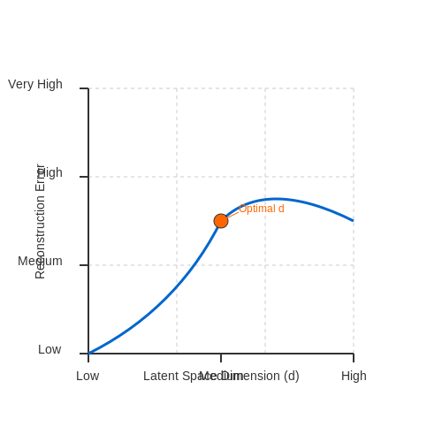
The dimensionality of the latent space in a Variational Autoencoder (VAE) is a critical hyperparameter that directly impacts model performance, interpretability, and computational efficiency. A poorly chosen latent dimension can lead to underfitting, overfitting, or inefficient representations. The optimal choice balances reconstruction fidelity with the complexity of the data manifold.
Theoretical Considerations
The latent space dimension d must be large enough to capture the intrinsic dimensionality of the data but small enough to avoid encoding noise. For a dataset with intrinsic dimensionality k, setting d < k forces the VAE to learn a compressed representation, potentially discarding useful information. Conversely, d >> k may lead to a degenerate posterior where the model ignores parts of the latent space.
The KL divergence term DKL penalizes deviations from the prior p(z), effectively regularizing the latent space. When d is too large, the model may minimize the KL term by collapsing posterior distributions to the prior, a phenomenon known as posterior collapse.
Empirical Methods for Dimension Selection
1. Eigenvalue Analysis of the Data Covariance Matrix
Compute the eigenvalues λi of the data covariance matrix and select d such that:
where τ is a threshold (e.g., 0.95) and D is the original data dimension. This ensures the latent space captures a sufficient fraction of the data variance.
2. Incremental Training with ELBO Monitoring
Train VAEs with increasing d and monitor the Evidence Lower Bound (ELBO). The point where the ELBO plateaus indicates diminishing returns from additional dimensions. This approach is computationally intensive but provides data-specific insights.
3. Nearest Neighbor Test
After training, sample points z from the latent space and decode them. If decoded samples from distinct z are perceptually identical, the latent space may be overparameterized. This qualitative test is useful for image data.
Practical Guidelines
- For natural images (e.g., 64×64 pixels), typical values range from d = 32 to 256.
- For structured data (e.g., tabular), start with d ≈ 0.1× input dimension.
- For sequential data, consider hierarchical latent spaces with varying dimensions per time step.
Recent work in disentangled representation learning suggests that higher latent dimensions can be beneficial when paired with appropriate regularization (e.g., β-VAE), but this increases training complexity.
Training VAEs: Practical Considerations
Optimizing the Evidence Lower Bound (ELBO)
The core training objective for VAEs is maximizing the Evidence Lower Bound (ELBO), which decomposes into a reconstruction term and a KL divergence term:
Here, β controls the trade-off between reconstruction fidelity and latent space regularization. For stable training:
- Annealing β: Start with β=0 and gradually increase to prevent latent collapse
- Warm-up periods: Linear scheduling over first 20% of training helps avoid local minima
- Free bits technique: Enforce minimum KL per dimension to prevent posterior collapse
Gradient Estimation and the Reparameterization Trick
Backpropagation through stochastic nodes requires special handling. For Gaussian latent variables:
Key implementation details:
- Numerical stability: Compute log-variance instead of variance to avoid NaN issues
- Gradient clipping: Limit norms to 1.0-5.0 prevents exploding gradients
- Variance reduction: Use control variates or multiple samples (≥3) for lower variance
Architectural Choices
The decoder and encoder architectures significantly impact performance:
| Component | Recommendation | Rationale |
|---|---|---|
| Encoder | ResNet blocks with spectral normalization | Stabilizes gradient flow |
| Decoder | PixelCNN++ or StyleGAN-like | Captures complex distributions |
| Latent Space | 32-256 dimensions | Balances expressivity and trainability |
Monitoring Training Dynamics
Essential metrics to track during training:
Where τ is a threshold (typically 0.01). Additional diagnostics:
- Reconstruction FID: Measures quality of generated samples
- Rate-Distortion curves: Plots reconstruction error vs KL term
- Latent traversals: Visualize semantic changes along principal axes
Advanced Regularization Techniques
Beyond basic KL regularization:
Where:
- Maximum Mean Discrepancy (MMD): Enforces aggregate posterior matching
- Total Correlation (TC): Encourages factorized latent representations
- Adversarial regularization: Uses a discriminator to improve sample quality
Hardware and Computational Considerations
For large-scale VAE training:
- Mixed precision: FP16 for activations, FP32 for master weights
- Gradient accumulation: Enables larger effective batch sizes
- Distributed training: Data parallelism with synchronized BatchNorm
4. Conditional VAEs and Their Use Cases
Conditional VAEs and Their Use Cases
Conditional Variational Autoencoders (CVAEs) extend the standard VAE framework by incorporating auxiliary information y (e.g., class labels, attributes, or structured metadata) into both the encoder and decoder. The joint distribution becomes p(x, z|y) = p(x|z, y)p(z|y), enabling controlled generation and inference conditioned on y. The evidence lower bound (ELBO) for CVAEs modifies the standard VAE objective:
Here, qϕ(z|x,y) is the conditional encoder, and pθ(x|z,y) is the conditional decoder. The hyperparameter β controls the trade-off between reconstruction fidelity and latent space regularization, analogous to the β-VAE framework.
Architectural Modifications
CVAEs integrate conditioning variables via concatenation or cross-attention mechanisms. For a label y encoded as a one-hot vector:
- The encoder input becomes [x, y], where x is the input data.
- The decoder receives [z, y] as input, ensuring generation adheres to the specified condition.
In practice, this is implemented by augmenting fully connected or convolutional layers to process the concatenated inputs. For high-dimensional conditions (e.g., text or images), embedding layers or transformers map y to a dense representation before fusion.
Key Use Cases
Controlled Data Generation
CVAEs enable precise generation of samples with desired attributes. In medical imaging, conditioning on lesion type (e.g., tumor grade) allows synthetic data generation for rare conditions. The model learns to disentangle pathological features from anatomical variations, improving downstream classifier robustness.
Missing Data Imputation
When applied to datasets with partial observations, CVAEs infer missing features xmiss given observed features xobs and metadata y. The conditional latent space captures correlations between observed and missing variables, yielding more accurate imputations than unconditional VAEs.
Cross-Modal Translation
By conditioning on modality descriptors (e.g., "MRI" or "CT"), CVAEs translate between imaging modalities while preserving anatomical structures. The decoder learns modality-specific rendering, enabling applications like synthetic CT generation from MRI inputs for radiation therapy planning.
Mathematical Derivation: Conditional Latent Space
The conditional prior p(z|y) is typically assumed Gaussian with parameters predicted from y:
where μ(y) and σ(y) are neural networks. The KL divergence term in the ELBO becomes:
with k the latent dimension. This formulation encourages the encoder to align with the conditional prior, structuring the latent space according to semantic attributes.
Advanced Variants
Recent extensions improve CVAE expressiveness:
- Hierarchical CVAEs stack multiple latent layers conditioned on y, capturing fine-grained attribute dependencies.
- Adversarial CVAEs add a discriminator to enforce sharper conditional distributions, mitigating blurry outputs.
- Discrete CVAEs employ categorical latent variables for structured conditions (e.g., parse trees in NLP).

Disentangled Representations in VAEs
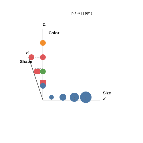
Disentangled representations in variational autoencoders (VAEs) refer to latent spaces where distinct dimensions correspond to independent generative factors of the data. This property is highly desirable for interpretability, robustness, and controllable generation. Formally, a disentangled representation satisfies:
where z is the latent vector of dimension d. This factorization implies statistical independence among latent dimensions.
Measuring Disentanglement
Several metrics quantify disentanglement quality:
- FactorVAE metric: Measures how well each latent dimension captures a single ground-truth factor through a majority vote classifier
- Mutual Information Gap (MIG): Computes the normalized difference between the top two latent dimensions with highest mutual information for each factor
- Separated Attribute Predictability (SAP): Uses linear classifiers to predict factors from individual latent dimensions
Methods for Achieving Disentanglement
β-VAE
The β-VAE introduces a hyperparameter β that weights the KL divergence term in the ELBO:
Higher β values (typically β > 1) encourage more factorized latent representations at the potential cost of reconstruction quality.
FactorVAE
FactorVAE augments the VAE objective with an additional total correlation (TC) term:
where DTC is estimated using density ratio estimation and measures the dependence between latent dimensions.
β-TCVAE
This approach decomposes the KL term into three components:
representing the index-code mutual information, total correlation, and dimension-wise KL divergence respectively. The β-TCVAE allows independent weighting of these terms.
Practical Considerations
In practice, achieving good disentanglement requires:
- Careful tuning of the β or γ hyperparameters
- Sufficient model capacity to maintain reconstruction quality
- Datasets with clearly separable generative factors
- Appropriate latent space dimensionality (neither too small nor too large)
Recent work has shown that unsupervised disentanglement is fundamentally impossible without inductive biases, as there are infinitely many equivalent factorizations of any distribution. Semi-supervised approaches that leverage limited labeled data often achieve better results.
Applications of Disentangled VAEs
Disentangled representations enable several advanced applications:
- Controllable generation: Modifying specific latent dimensions to alter single attributes in generated samples
- Few-shot learning: Rapid adaptation to new tasks by recombining learned factors
- Domain adaptation: Transferring learned factors across different but related domains
- Interpretable representations: Human-understandable decomposition of data variation
4.3 VAEs for Anomaly Detection and Data Generation
Anomaly Detection with VAEs
Variational Autoencoders excel in anomaly detection by leveraging their probabilistic latent space. Unlike deterministic autoencoders, VAEs model the data distribution p(x) explicitly, allowing for principled outlier detection. The reconstruction probability, derived from the evidence lower bound (ELBO), serves as a robust anomaly score:
Anomalies are identified when the reconstruction probability falls below a threshold. The Mahalanobis distance in the latent space z further refines detection:
where μ and Σ are the mean and covariance of the latent distribution. This approach is particularly effective in high-dimensional data like medical imaging or industrial sensor data, where anomalies are rare but critical.
Data Generation via Latent Space Interpolation
VAEs generate data by sampling from the prior p(z) = N(0, I) and decoding via p_θ(x|z). The smoothness of the latent space enables meaningful interpolations between data points. For two latent vectors z_1 and z_2, linear interpolation yields:
This property is exploited in applications like molecular design and synthetic image generation, where VAEs produce novel samples that preserve data manifold constraints.
Conditional VAEs for Controlled Generation
Conditional VAEs (CVAEs) extend the framework by incorporating labels y into both encoder and decoder:
The ELBO for CVAEs modifies the standard VAE objective:
CVAEs enable targeted generation, such as creating specific drug compounds or fault scenarios in mechanical systems, by conditioning on desired attributes.
Practical Implementation Considerations
- Latent Space Regularization: The KL divergence term must be carefully weighted (e.g., via β-VAE) to avoid posterior collapse.
- Anomaly Thresholding: The reconstruction probability threshold is typically set using extreme value theory or quantile analysis on validation data.
- Evaluation Metrics: For generation, use Frechet Inception Distance (FID) or precision/recall for manifolds; for anomaly detection, leverage AUROC or F1-score.
Below is a PyTorch snippet for computing the reconstruction probability anomaly score:
def anomaly_score(model, x, n_samples=100):
    model.eval()
    with torch.no_grad():
        # Monte Carlo estimate of reconstruction probability
        recon_probs = []
        for _ in range(n_samples):
            x_recon, μ, logvar = model(x)
            log_prob = -F.mse_loss(x_recon, x, reduction='none').sum(dim=[1,2,3])
            recon_probs.append(log_prob)
        recon_prob = torch.logsumexp(torch.stack(recon_probs), dim=0) - np.log(n_samples)
    return -recon_prob  # Higher score = more anomalous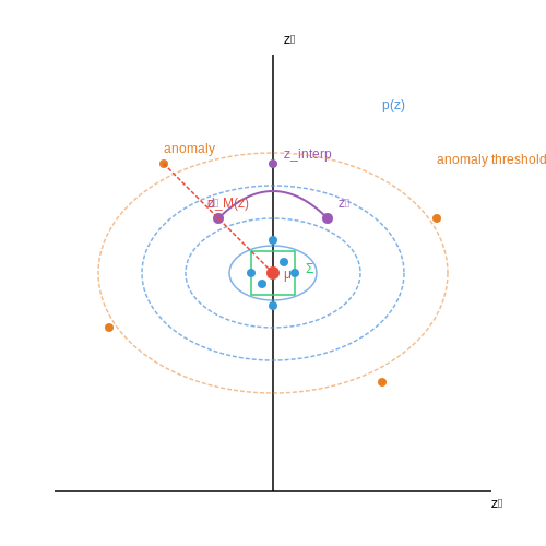
5. Mode Collapse and How to Mitigate It
Mode Collapse and How to Mitigate It
Mode collapse occurs when a VAE generates a limited subset of the data distribution, ignoring other valid modes. This phenomenon arises because the model optimizes for the average case, often converging to a single or few high-likelihood outputs rather than capturing the full diversity of the training data. The issue is particularly prevalent when the latent space is under-regularized or the decoder is too powerful relative to the encoder.
Mathematical Underpinnings
The ELBO (Evidence Lower Bound) objective of a VAE is given by:
When mode collapse occurs, the KL divergence term \( D_{KL}(q_\phi(z|x) \parallel p(z)) \) becomes negligible, allowing the decoder to exploit a small region of the latent space. This results in the model generating similar outputs regardless of the input.
Common Causes
- High-capacity decoders: Overpowered decoders can reconstruct data with minimal reliance on the latent space, bypassing meaningful representations.
- Weak regularization (low \(\beta\)): Insufficient pressure to structure the latent space leads to poor disentanglement and mode collapse.
- Imbalanced datasets: If certain modes dominate the training data, the model may prioritize these over rarer ones.
Mitigation Strategies
1. Adjusting the KL Weight (\(\beta\))
Increasing \(\beta\) in the \(\beta\)-VAE framework strengthens the regularization effect, forcing the latent space to better align with the prior \( p(z) \). However, setting \(\beta\) too high can lead to posterior collapse, where the latent variables become uninformative.
2. Using a More Expressive Prior
Replacing the standard Gaussian prior with a more flexible distribution, such as a mixture of Gaussians, can help capture multi-modal data:
3. Adversarial Training
Incorporating a discriminator network, as in Adversarial Autoencoders (AAEs), encourages the aggregated posterior \( q(z) \) to match the prior \( p(z) \), reducing mode collapse:
4. Minibatch Discrimination
By comparing samples within a minibatch, the model is penalized for generating similar outputs, promoting diversity. This technique, borrowed from GANs, can be adapted for VAEs.
5. Auxiliary Loss Functions
Adding auxiliary losses, such as reconstruction penalties for diverse outputs or mutual information maximization, can prevent the model from collapsing to a single mode.
Practical Considerations
In practice, monitoring the diversity of generated samples during training is essential. Techniques like Fréchet Inception Distance (FID) or precision-recall metrics for generative models can quantify mode collapse. Early stopping or dynamic adjustment of \(\beta\) based on these metrics can further stabilize training.
5.2 Balancing Reconstruction and Regularization
The core challenge in training variational autoencoders lies in optimizing the evidence lower bound (ELBO), which decomposes into two competing terms:
The Reconstruction-Regularization Tradeoff
The first term measures reconstruction quality through the expected log-likelihood of the data given latent samples. The second term acts as a regularizer, pushing the approximate posterior qφ(z|x) toward the prior p(z) (typically isotropic Gaussian). These objectives often conflict:
- Perfect reconstruction requires the latent space to preserve all data details, potentially ignoring the prior
- Strict regularization forces latent codes to match a simple distribution, potentially losing input information
β-VAE: Explicit Balance Control
The β parameter explicitly weights the KL term's influence. Practical considerations emerge:
Empirical studies show β=1 works for many datasets, but structured data often benefits from β∈[0.1, 0.5]. The β-VAE framework enables controlled exploration of this trade space.
Alternative Approaches
Free Bits Technique
Instead of global weighting, constrain the KL term per latent dimension:
where λ sets a minimum required KL value per dimension, preventing complete collapse while allowing adaptive compression.
Cyclical Annealing
Gradually introduce KL pressure via a scheduled weight α(t):
where T controls the warmup period. This lets the model learn useful representations before regularization dominates.
Practical Implications
In image generation tasks, reconstruction quality typically requires:
- Higher-capacity decoders
- Lower β values (0.1-0.5 range)
- Latent dimensions ≥128 for complex data
For disentangled representation learning, opposite settings work better:
- Bottleneck architectures
- β values 4-10
- Lower-dimensional latent spaces
The optimal balance depends on downstream use: generation tasks tolerate higher reconstruction error for better latent structure, while compression applications prioritize accurate reconstructions.
5.3 Scalability Issues in High-Dimensional Spaces
Variational Autoencoders (VAEs) face significant challenges when operating in high-dimensional spaces, primarily due to the curse of dimensionality and the computational complexity of approximating posterior distributions. As the dimensionality of the input space grows, the latent space must capture increasingly intricate structures, leading to inefficiencies in both training and inference.
Posterior Collapse and Latent Space Dilution
In high dimensions, the VAE's encoder often fails to learn meaningful latent representations, a phenomenon known as posterior collapse. This occurs when the approximate posterior $$q_\phi(z|x)$$ collapses to the prior $$p(z)$$, rendering the latent variables uninformative. The Kullback-Leibler (KL) divergence term in the ELBO objective:
can dominate the reconstruction loss, especially when the decoder $$p_\theta(x|z)$$ is overly expressive. Mitigation strategies include:
- KL annealing: Gradually increasing the weight of the KL term during training.
- Modified architectures: Using hierarchical latent spaces or auxiliary loss terms.
Computational Bottlenecks in High Dimensions
The sampling process in VAEs involves generating latent vectors $$z \sim q_\phi(z|x)$$, which becomes computationally expensive in high-dimensional spaces. The reparameterization trick:
requires $$O(d)$$ operations for a $$d$$-dimensional latent space, leading to scalability issues. Parallelization and sparse variational approximations can alleviate this, but trade-offs between fidelity and efficiency persist.
Dimensionality Reduction Techniques
To combat these issues, practitioners often employ:
- Principal Component Analysis (PCA): Preprocessing data to reduce input dimensionality.
- Stochastic Neighborhood Embedding (t-SNE): Visualizing latent spaces to diagnose collapse.
- Normalizing Flows: Enhancing the flexibility of $$q_\phi(z|x)$$ through invertible transformations.
Case Study: Image Generation at Scale
In large-scale image generation (e.g., $$1024 \times 1024$$ pixels), VAEs struggle with:
- Memory constraints: Storing high-resolution feature maps in the encoder/decoder.
- Gradient instability: Vanishing or exploding gradients due to deep architectures.
Recent work leverages vector-quantized VAEs (VQ-VAEs), which discretize the latent space to improve scalability while preserving perceptual quality.
where $$z_q(x)$$ is the quantized latent vector, $$z_e(x)$$ is the encoder output, and $$\text{sg}$$ denotes the stop-gradient operation.

6. Foundational Papers on VAEs
6.1 Foundational Papers on VAEs
- [1906.02691] An Introduction to Variational Autoencoders - arXiv.org — Variational autoencoders provide a principled framework for learning deep latent-variable models and corresponding inference models. ... We gratefully acknowledge support from the Simons Foundation, member institutions, and all contributors ... View a PDF of the paper titled An Introduction to Variational Autoencoders, by Diederik P. Kingma and ...
- Variations in Variational Autoencoders - IEEE Xplore — Variational Auto-Encoders (VAEs) are deep latent space generative models which have been immensely successful in many applications such as image generation, image captioning, protein design, mutation prediction, and language models among others. The fundamental idea in VAEs is to learn the distribution of data in such a way that new meaningful data can be generated from the encoded ...
- An Overview of Variational Autoencoders for Source Separation, Finance ... — Variational Autoencoders (VAEs) can be regarded as enhanced Autoencoders where a Bayesian approach is used to learn the probability distribution of the input data. VAEs have found wide applications in generating data for speech, images, and text. In this paper, we present a general comprehensive overview of variational autoencoders.
- Variational Autoencoders - Theory and Applications: Exploring ... — Variational autoencoders (VAEs) have emerged as a powerful framework for generative modeling and representation learning in recent years. This paper provides a comprehensive overview of VAEs, starting with their theoretical foundations and then exploring their diverse applications. We begin by explaining the basic principles of VAEs, including the encoder and decoder networks, the ...
- An Introduction to Variational Autoencoders - IEEE Xplore — Abstract: In this monograph, the authors present an introduction to the framework of variational autoencoders (VAEs) that provides a principled method for jointly learning deep latent-variable models and corresponding inference models using stochastic gradient descent. The framework has a wide array of applications from generative modeling, semi-supervised learning to representation learning.
- PDF Structured VAEs: Composing Probabilistic Graphical Models and ... — 2.2. Variational autoencoders The variational autoencoder (VAE) (Kingma & Welling, 2014;Rezende et al.,2014) is a recent model and varia-tional inference method that links neural network autoen-coders (Vincent et al.,2008) with mean field variational Bayes. Given a high-dimensional dataset y = fy ngN =1
- PDF Dynamical Variational Autoencoders: A Comprehensive Review — Dynamical Variational Autoencoders: A Comprehensive Review Laurent Girin, Simon Leglaive, Xiaoyu Bie, Julien Diard, Thomas Hueber, ... Variational autoencoders (VAEs) are powerful deep gen- ... in the original papers. Finally, we present the corresponding VLB. ...
- Exploring Variational Autoencoders and Generative Latent Time-Series ... — This study examines the fundamental theory necessary for comprehending Variational Autoencoders (VAEs) and generative latent time-series models. We will also explain how these models extend the principles of VAEs to the domain of time-series data by incorporating temporal dependencies into the latent space. By leveraging the probabilistic nature of VAEs and the temporal dependencies captured ...
- Variations in Variational Autoencoders - A Comparative Evaluation — Variational Auto-Encoders (VAEs) are deep latent space generative models which have been immensely successful in many applications such as image generation, image captioning, protein design, mu ...
- PDF Approximate Inference in Variational Autoencoders - Chris Cremer — approximate inference in VAEs. This thesis reviews many of the recent developments made to improve VAEs. One such improvement is the importance-weighted autoencoder. The standard interpretation of importance-weighted autoencoders is that they maximize a tighter lower bound on the marginal likelihood than the standard evidence lower bound.
6.2 Books and Comprehensive Guides
- 16 Variational autoencoders | Applied deep learning with torch from R — 16 Variational autoencoders. Now we look at the other - as of this writing - main type of architecture used for self-supervised learning: Variational Autoencoders (VAEs). VAEs are autoencoders, in that they compress their input and, starting from a compressed representation, aim for a faithful reconstruction. But in addition, there is a ...
- Variational Autoencoders: How They Work and Why They Matter — Variational Autoencoders (VAEs) are used for generating new, high-quality data samples, making them valuable in applications like image synthesis and data augmentation. They are also employed in anomaly detection, where they identify deviations from learned data distributions and in data denoising and imputation by reconstructing missing or ...
- Autoencoders, Variational Autoencoders (VAE) and β-VAE — Autoencoders (AE), Variational Autoencoders (VAE), and β-VAE are all generative models used in unsupervised learning. Regardless of the architecture, all these models have so-called encoder and…
- Variational autoencoder - Wikipedia — In machine learning, a variational autoencoder (VAE) is an artificial neural network architecture introduced by Diederik P. Kingma and Max Welling. [1] It is part of the families of probabilistic graphical models and variational Bayesian methods. [2]In addition to being seen as an autoencoder neural network architecture, variational autoencoders can also be studied within the mathematical ...
- Variational AutoEncoders - GeeksforGeeks — Variational Autoencoders (VAEs) are generative models in machine learning (ML) that create new data similar to the input they are trained on. Along with data generation they also perform common autoencoder tasks like denoising. Like all autoencoders VAEs consist of: Encoder: Learns important patterns (latent variables) from input data.
- A Hands-On Guide to Building and Training Variational Autoencoders — VAEs are a type of generative model that can be used to generate images, compress data, and detect anomalies. They are based on the concept of "autoencoders," which are neural networks that can ...
- What is a Variational Autoencoder? - IBM — Like all autoencoders, variational autoencoders are deep learning models composed of an encoder that learns to isolate the important latent variables from training data and a decoder that then uses those latent variables to reconstruct the input data. However, whereas most autoencoder architectures encode a discrete, fixed representation of latent variables, VAEs encode a continuous ...
- An Overview of Variational Autoencoders for Source Separation, Finance ... — Autoencoders are a self-supervised learning system where, during training, the output is an approximation of the input. Typically, autoencoders have three parts: Encoder (which produces a compressed latent space representation of the input data), the Latent Space (which retains the knowledge in the input data with reduced dimensionality but preserves maximum information) and the Decoder (which ...
- Variational autoencoders. - Jeremy Jordan — In my introductory post on autoencoders, I discussed various models (undercomplete, sparse, denoising, contractive) which take data as input and discover some latent state representation of that data. More specifically, our input data is converted into an encoding vector where each dimension represents some learned attribute about the data. The most important detail to grasp here is that our ...
6.3 Online Resources and Tutorials
- An Introduction To Variational Autoencoders: Foundations and ... - Scribd — 1906.02691 - Free download as PDF File (.pdf), Text File (.txt) or read online for free. This document provides an introduction to variational autoencoders (VAEs). VAEs provide a principled framework for learning deep latent variable models and corresponding inference models. The document discusses the motivation for generative modeling and variational inference.
- A deep dive into conditional variational autoencoders — VAEs - despite their conceptual simplicity - can be difficult to understand and even more so for its conditional variants. ... An introduction to variational autoencoders. Foundations and Trends in Machine Learning, 12(4), 307-392. kingma2019introduction Kingma, D. P., Welling, M., & others, (2019). An introduction to variational ...
- The Reparameterization Trick in Variational Autoencoders — We first provide a quick refresher on variational autoencoders (VAEs). We then explain why the VAE needs the reparameterization trick, what the trick is and how to implement it. After explaining the use of the trick we justify it formally. 2. Variational Autoencoders
- Variational autoencoders - Matthew N. Bernstein — Variational autoencoders (VAEs) are a family of deep generative models with use cases that span many applications, from image processing to bioinformatics. There are two complimentary ways of viewing the VAE: as a probabilistic model that is fit using variational Bayesian inference, or as a type of autoencoding neural network. In this post, we present the mathematical theory behind VAEs, which ...
- Variational Autoencoder with Global- and Medium Timescale ... - Springer — Variational autoencoders (VAEs) are generative unsupervised learning models that create low-dimensional representations of the input data and learn by regenerating the same input from that representation. Recently, VAEs were used to extract representations from audio data, which possess not only content-dependent information but also speaker ...
- Variational Autoencoders with Keras and MNIST — The goals of this notebook is to learn how to code a variational autoencoder in Keras. We will discuss hyperparameters, training, and loss-functions. In addition, we will familiarize ourselves with the Keras sequential GUI as well as how to visualize results and make predictions using a VAE with a small number of latent dimensions.
- Artificial Intelligence - Part 7.3 - GENERATIVE AI - VAEs - LinkedIn — Variational Autoencoders (VAEs) are a powerful class of generative models in machine learning that combine principles from neural networks and probability theory.
- Lecture 6.3: Variational Auto-Encoders - YouTube — In the last video of the lecture on Deep Generative Modeling, we introduce and explain Variational Auto-Encoders. We derive the learning objective (Evidence ...
- An Overview of Variational Autoencoders for Source Separation, Finance ... — Abstract. Autoencoders are a self-supervised learning system where, during training, the output is an approximation of the input. Typically, autoencoders have three parts: Encoder (which produces a compressed latent space representation of the input data), the Latent Space (which retains the knowledge in the input data with reduced dimensionality but preserves maximum information) and the ...
- An Overview of Variational Autoencoders for Source Separation, Finance ... — Autoencoders are a self-supervised learning system where, during training, the output is an approximation of the input. Typically, autoencoders have three parts: Encoder (which produces a compressed latent space representation of the input data), the Latent Space (which retains the knowledge in the input data with reduced dimensionality but preserves maximum information) and the Decoder (which ...







