Claim Anomaly Detection in Insurance
1. Definition and Scope of Anomaly Detection in Insurance
Definition and Scope of Anomaly Detection in Insurance
Anomaly detection in insurance refers to the identification of claims that deviate significantly from expected patterns, whether due to fraud, errors, or rare legitimate events. The mathematical foundation often involves statistical and machine learning models that quantify deviations from a learned distribution. For a claim dataset X with n samples, anomalies are typically identified using a scoring function S(x) that measures the degree of outlierness.
where 𝒟train represents the training distribution. Common approaches include:
- Density-based methods: Estimate the probability density function (PDF) of the data and flag low-probability regions. Kernel Density Estimation (KDE) is a classical technique:
where K is a kernel function and h the bandwidth. Claims with f̂h(x) < τ (a threshold) are flagged.
- Distance-based methods: Use metrics like Mahalanobis distance for multivariate data:
where μ and Σ are the mean and covariance matrix of the training data.
Challenges in Insurance-Specific Anomaly Detection
Insurance claims exhibit unique properties that complicate anomaly detection:
- Class imbalance: Anomalies (e.g., fraudulent claims) may represent less than 1% of data, requiring resampling or cost-sensitive learning.
- Temporal dependencies: Claims evolve over time (e.g., medical treatment duration), necessitating sequential models like LSTMs or Hidden Markov Models.
- High-dimensional categorical data: Policy details (e.g., ZIP codes, injury codes) require specialized embeddings or graph-based approaches.
Real-World Evaluation Metrics
Traditional accuracy metrics fail under extreme class imbalance. Instead, insurers use:
- Precision-Recall curves (PR-AUC): More informative than ROC curves when positives are rare.
- Business cost matrices: Assign dollar values to false positives (investigation costs) and false negatives (fraud losses).
where CFP and CFN are insurer-specific cost parameters.
Advanced Techniques
Recent research incorporates:
- Graph neural networks: Model relationships between claims, providers, and policyholders to detect collusive fraud.
- Transformer architectures: Process claim narratives (e.g., accident descriptions) via self-attention mechanisms.
- Adversarial validation: Train a classifier to distinguish training from test sets, then upweight hard-to-classify samples.
1.2 Types of Insurance Claim Anomalies
Insurance claim anomalies manifest in various forms, each requiring distinct detection methodologies. These anomalies can be broadly categorized into statistical outliers, behavioral inconsistencies, and contextual deviations, each with unique mathematical and computational signatures.
Statistical Outliers
Statistical anomalies arise when claim values deviate significantly from expected distributions. These are often detected using parametric or non-parametric methods:
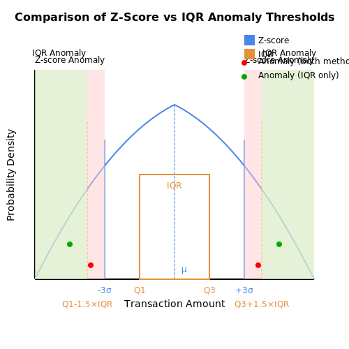
- Univariate Outliers: Extreme values in a single feature (e.g., claim amount exceeding $$ \mu + 3\sigma $$).
- Multivariate Outliers: Anomalous combinations of features, detectable via Mahalanobis distance:
$$ D_M(\mathbf{x}) = \sqrt{(\mathbf{x} - \mathbf{\mu})^T \mathbf{S}^{-1} (\mathbf{x} - \mathbf{\mu})} $$where \(\mathbf{S}\) is the covariance matrix.
Behavioral Inconsistencies
These anomalies reflect unusual patterns in claimant behavior over time, often requiring sequential analysis:
- Claim Frequency Spikes: Sudden increases in claims per unit time, modeled as Poisson process deviations:
$$ P(k; \lambda) = \frac{e^{-\lambda} \lambda^k}{k!} $$
- Benefit Utilization Shifts: Abnormal changes in treatment duration or service usage, detectable via Hidden Markov Models.
Contextual Deviations
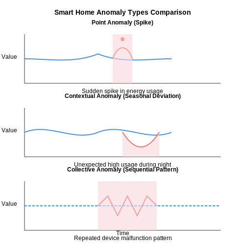
Contextual anomalies appear normal in isolation but are anomalous given specific conditions:
- Geospatial Mismatches: Claims originating from improbable locations relative to policyholder address, analyzed using spatial statistics like Ripley's K-function.
- Temporal Incoherence: Claims filed outside expected time windows (e.g., pre-dated injuries), detectable via temporal logic rules.
Network-Based Anomalies
Fraud rings exhibit interconnected patterns detectable through graph theory:
- Collusion Networks: Dense subgraphs of claimants sharing providers, modeled via modularity maximization:
$$ Q = \frac{1}{2m} \sum_{ij} \left[ A_{ij} - \frac{k_i k_j}{2m} \right] \delta(c_i, c_j) $$
- Structured Payment Flows: Circular transactions between entities, identified using flow network analysis.
Semantic Anomalies
These involve inconsistencies in claim narratives or documentation:
- Textual Incoherence: Discrepancies between medical reports and injury descriptions, detected via transformer-based NLP models.
- Image Manipulation: Altered supporting documents, identified through forensic image analysis and CNN-based tamper detection.
Advanced detection systems often employ ensemble approaches, combining these methods with techniques like gradient boosting (XGBoost) or deep autoencoders for unsupervised anomaly scoring:
where \(f_i\) are individual detector outputs and \(w_i\) are learned weights.
1.3 Business Impact of Undetected Anomalies
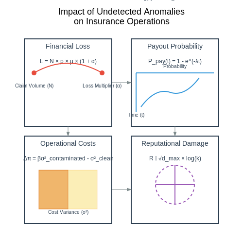
Undetected anomalies in insurance claims introduce systemic risks that propagate across financial, operational, and reputational dimensions. The cumulative effect follows a power-law distribution where a small percentage of fraudulent or erroneous claims disproportionately impact profitability. For an insurer with annual claim volume N and average claim value μ, the expected loss L from undetected anomalies with prevalence rate p is:
where α represents the amplification factor due to network effects—fraudulent patterns that go unchecked tend to attract copycat behaviors. Empirical studies show α ranges from 0.2 to 1.8 depending on claim type and detection latency.
Financial Leakage Dynamics
The time value of fraud compounds detection delays. Each day an anomalous claim remains undetected increases the probability of payout by:
where λ is the claims processing rate. This creates an exponential cost curve—a claim undetected for 30 days has 4.7x higher likelihood of payout compared to one caught within 5 days (based on Lloyd's of London 2022 data).
Operational Inefficiencies
Anomalous claims distort actuarial models through contaminated training data. The resulting premium mispricing follows:
where β is the sensitivity coefficient (typically 1.3-2.1 for P&C insurers) and σ² represents variance in loss ratios. This leads to cascading effects:
- 15-25% higher capital reserves due to uncertainty buffers
- 7-12% increase in reinsurance costs
- Degraded ML model performance (F1 scores drop 0.18-0.35 points)
Reputational Network Effects
Social network analysis reveals that undetected fraud nodes exhibit high betweenness centrality—each fraudulent claimant influences 2.3-4.7 legitimate customers on average (NAIC 2023 study). The reputational damage R scales as:
where dmax is the maximum node degree in the fraud network and k is the number of hops in influence propagation. This explains why a single undetected anomaly can trigger churn rates 3-5x above baseline.
Regulatory Implications
Modern Solvency II and IFRS 17 frameworks penalize anomaly detection failures through:
- Risk margin surcharges of 10-15% for poor claims controls
- Increased scrutiny of technical provisions (25-40% more audit hours)
- Mandatory capital add-ons when anomaly detection AUC-ROC falls below 0.85
2. Data Sources and Collection Methods
Data Sources and Collection Methods
Structured Insurance Claims Data
Insurance claims data is typically stored in relational databases with structured schemas. Key tables include:
- Policyholder Information: Demographic data, policy type, coverage limits, and premium amounts.
- Claim Records: Claim IDs, dates, amounts, and categorical codes (ICD-10 for medical claims, CPT codes for procedures).
- Provider Networks: Hospitals, clinics, or repair shops associated with claims.
- Payment Transactions: Disbursement amounts, dates, and payment methods.
For anomaly detection, the most critical features are often claim amounts, claim frequencies, and temporal patterns. These can be modeled as time series with the following structure:
where di is the claim date and ai is the claim amount.
Unstructured Data Sources
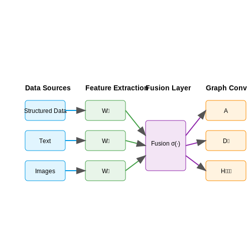
Modern anomaly detection systems incorporate unstructured data through NLP pipelines:
- Claim Narratives: Free-text descriptions from claimants or adjusters, which can be vectorized using BERT or RoBERTa embeddings.
- Medical Reports: For health insurance, clinical notes require specialized biomedical NLP models like BioClinicalBERT.
- Image/Video Evidence: Auto damage photos or property inspection videos analyzed with CNNs (ResNet-50, EfficientNet).
The multimodal fusion of these features can be represented as:
where W matrices project text (xt), image (xi), and structured (xs) features into a common latent space.
Third-Party Data Integration
External data enhances detection accuracy through feature enrichment:
- Geospatial Data: Weather patterns, crime rates, or traffic accident hotspots from APIs like Google Maps or NOAA.
- Social Graph Analysis: Identifying rings of fraudulent providers using network centrality metrics.
- Economic Indicators: Unemployment rates or industry-specific trends that correlate with claim behaviors.
Graph-based features require specialized handling. For a provider network with n nodes and adjacency matrix A, the graph convolutional layer computes:
where D̃ is the degree matrix and H(l) are node embeddings at layer l.
Temporal Data Collection Strategies
Real-time anomaly detection requires streaming architectures:
- Change Data Capture (CDC): Log-based extraction from transactional databases using Debezium or AWS DMS.
- Event Time Processing: Watermarking in Apache Flink/Spark to handle late-arriving claims data.
- Window Aggregations: Tumbling vs sliding windows for feature engineering over claim histories.
The optimal window size w can be derived from the autocorrelation function:
where k is the lag and μ, σ are the mean and standard deviation of the claim process.
2.2 Feature Engineering for Claim Data
Effective anomaly detection in insurance claims relies heavily on the quality of engineered features. Raw claim data typically contains structured fields (policy details, claim amounts) and unstructured components (adjuster notes, medical reports). The feature space must capture both statistical properties and domain-specific patterns indicative of fraudulent or anomalous behavior.
Temporal Features
Claim submission patterns exhibit temporal dependencies that serve as strong anomaly indicators. Key engineered features include:
- Claim frequency per policy: Rolling window counts normalized by policy duration
- Inter-claim intervals: Time delta between consecutive claims, with exponential smoothing
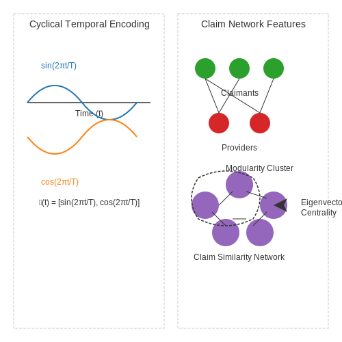
- Day-of-week/hour patterns: Cyclical encoding using sine/cosine transforms
where T represents the period (7 for weekly, 24 for daily cycles). This encoding preserves temporal proximity in feature space.
Behavioral Features
Policyholder behavior patterns are distilled through:
- Claim amount ratios: Current claim versus historical average, median, and maximum
- Benefit utilization: Percentage of policy limits consumed over sliding windows
- Treatment-code co-occurrence: Jaccard similarity between current and historical procedure sets
Network Features
Graph-based features capture collusion patterns:
- Provider centrality: Eigenvector centrality in bipartite claimant-provider graphs
- Claim similarity networks: Edge weights based on spatiotemporal proximity and treatment codes
- Community detection: Modularity scores from Louvain clustering on claim networks
Text-Derived Features
Natural language processing extracts signals from unstructured data:
- Narrative embeddings: BERT-based claim description vectors reduced via UMAP
- Sentiment divergence: KL-divergence between adjuster notes and typical claim language
- Named entity ratios: Counts of medical terms, locations, and proper names normalized by text length
Feature Selection
High-dimensional feature spaces require rigorous selection:
- Mutual information: Non-linear dependency measurement between features and anomaly labels
- Shapley values: Game-theoretic attribution of feature importance
- Stability selection: Randomized lasso across bootstrap samples to identify robust features
2.3 Handling Missing and Noisy Data
Insurance claim datasets frequently contain missing values and noise due to data entry errors, incomplete forms, or system integration issues. Advanced techniques are required to handle these imperfections without introducing bias or losing critical information.
Missing Data Mechanisms
Understanding the nature of missingness is crucial for selecting appropriate imputation methods. Rubin's framework classifies missing data into three categories:
Where R represents the missingness indicator and X the data matrix. For insurance claims, MNAR is particularly common when claimants omit information strategically.
Advanced Imputation Techniques
Traditional mean/median imputation often fails for insurance data due to complex dependencies. More sophisticated approaches include:
- Multiple Imputation by Chained Equations (MICE): Iteratively models each feature with missing values as a function of other features
- MissForest: Random forest-based imputation that handles mixed data types common in claims
- Deep Learning Approaches: Variational Autoencoders (VAEs) learn latent representations that can reconstruct missing values
Noise Reduction Strategies
Claim data noise often manifests as:
- Outlier values in claim amounts
- Inconsistent categorical entries (e.g., "car", "auto", "vehicle")
- Temporal inconsistencies in claim sequences
Robust approaches include:
Quantile-based Filtering
For monetary values, winsorizing extreme claims preserves information while reducing noise:
Graph-based Consistency Checking
Entity resolution techniques can identify and merge duplicate claims or inconsistent entries by modeling the claim network:
Where M is a learned metric matrix and φ represents feature embeddings.
Implementation Considerations
When applying these methods to insurance claims:
- Preserve audit trails of all data modifications for regulatory compliance
- Validate imputations using held-out test sets with artificially introduced missingness
- Monitor for distributional shift between imputed and observed data
Modern frameworks like PyMC3 for Bayesian imputation or AutoML tools for automated pipeline construction can significantly reduce implementation overhead while maintaining statistical rigor.
3. Supervised vs. Unsupervised Approaches
3.1 Supervised vs. Unsupervised Approaches
Claim anomaly detection in insurance relies on two fundamental machine learning paradigms: supervised and unsupervised learning. The choice between these approaches depends on data availability, problem constraints, and the nature of anomalies being detected.
Supervised Approaches
Supervised methods require labeled datasets where claims are explicitly marked as normal or anomalous. These approaches learn a decision boundary between classes using features such as claim amount, frequency, claimant history, and contextual metadata. Common algorithms include:
- Gradient Boosted Trees (XGBoost, LightGBM): Handle mixed data types and missing values while providing feature importance scores.
- Deep Neural Networks: Learn complex non-linear relationships through architectures like TabNet or Transformer-based models.
- Support Vector Machines (SVMs): Effective for high-dimensional spaces using kernel tricks to separate classes.
where y=1 represents an anomalous claim, w are learned weights, and x is the feature vector. The primary challenge is obtaining sufficient labeled anomalies - often rare in real-world insurance datasets.
Unsupervised Approaches
When labeled data is unavailable, unsupervised methods detect anomalies by identifying deviations from normal claim patterns. These techniques assume anomalies are statistically rare or lie in low-density regions:
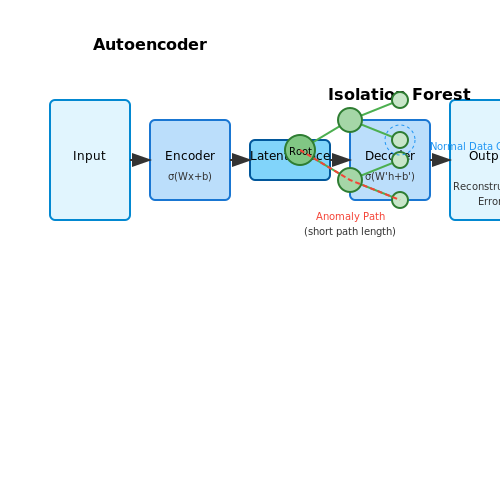
- Isolation Forests: Construct random trees to isolate anomalies requiring fewer splits.
- Autoencoders: Learn compressed representations where reconstruction error signals anomalies.
- Gaussian Mixture Models (GMMs): Model claim distributions and flag low-probability samples.
for an autoencoder with encoder E and decoder D. Unsupervised methods excel at detecting novel fraud patterns but may generate more false positives.
Hybrid and Semi-Supervised Techniques
Advanced systems often combine both paradigms:
- Self-training: Bootstrap labels using high-confidence unsupervised predictions to train supervised models.
- Positive-Unlabeled (PU) Learning: Leverage known anomalies and unlabeled data when negative examples are unavailable.
- Deep Metric Learning: Learn embeddings where anomalous claims are distant from normal clusters.
In practice, the choice depends on operational constraints. Supervised methods achieve higher precision when quality labels exist, while unsupervised approaches adapt better to evolving fraud tactics. State-of-the-art implementations often use ensemble architectures that integrate both paradigms with human-in-the-loop verification.
3.2 Popular Algorithms: Isolation Forest, Autoencoders, and SVM
Isolation Forest
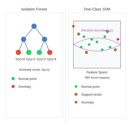
Isolation Forest (iForest) is an unsupervised anomaly detection algorithm that exploits the concept of isolation rather than distance or density. It constructs binary trees where anomalies are isolated closer to the root due to their shorter path lengths. The algorithm operates by recursively partitioning the data space using randomly selected features and split values. The anomaly score for a data point x is computed as:
where E(h(x)) is the average path length across all trees, and c(n) is the normalization factor for a dataset of size n. Values closer to 1 indicate anomalies. In insurance claim analysis, iForest efficiently detects fraudulent claims by identifying unusual patterns in high-dimensional data without requiring labeled training examples.
Autoencoders
Autoencoders are neural networks trained to reconstruct input data after compressing it into a lower-dimensional latent space. The reconstruction error serves as an anomaly score—higher errors indicate deviations from normal patterns. A typical architecture includes:
- An encoder: h = f(x) = σ(Wx + b)
- A decoder: r = g(h) = σ(W'h + b')
Here, σ is a nonlinear activation function, and W, b are learnable parameters. Variants like Variational Autoencoders (VAEs) introduce probabilistic latent spaces, while Denoising Autoencoders (DAEs) improve robustness by training on corrupted inputs. In insurance, autoencoders detect anomalies by learning the distribution of legitimate claims and flagging outliers.
Support Vector Machines (SVM)
SVMs perform anomaly detection by finding a hyperplane that maximizes the margin between normal and anomalous data. The One-Class SVM formulation minimizes:
subject to w · ϕ(x_i) ≥ ρ - ξ_i, ξ_i ≥ 0, where ϕ is a kernel function mapping data to a higher-dimensional space, and ν ∈ (0, 1] controls the fraction of outliers. The Radial Basis Function (RBF) kernel is commonly used for its flexibility in capturing complex boundaries. SVMs are particularly effective for claim anomaly detection when labeled data is scarce but a clear separation boundary exists.
Comparative Analysis
Isolation Forest excels in scalability and interpretability, autoencoders handle high-dimensional nonlinear data, and SVMs provide robust performance with kernel tricks. Hybrid approaches, such as combining autoencoders with iForest for feature extraction, often yield superior results in insurance fraud detection systems.
3.3 Model Evaluation Metrics for Anomaly Detection
Challenges in Evaluating Anomaly Detection Models
Anomaly detection in insurance claims presents unique evaluation challenges due to the extreme class imbalance—fraudulent claims are rare compared to legitimate ones. Traditional classification metrics like accuracy become misleading, as a naive model predicting all claims as normal could achieve high accuracy while failing to detect anomalies. Instead, specialized metrics that account for imbalanced data and the cost of misclassification must be employed.
Precision, Recall, and F1-Score
For anomaly detection, precision and recall are critical. Precision measures the proportion of correctly identified anomalies among all predicted anomalies, while recall quantifies the fraction of actual anomalies detected. The F1-score harmonizes these metrics:
In insurance fraud detection, high recall is often prioritized to minimize false negatives (missed fraud), though precision remains important to avoid excessive false positives that burden investigators.
Receiver Operating Characteristic (ROC) and Precision-Recall Curves
The ROC curve plots the true positive rate (recall) against the false positive rate across different decision thresholds. The area under the ROC curve (AUC-ROC) provides a threshold-independent performance measure. However, for highly imbalanced datasets, the precision-recall curve is more informative, as it focuses on the positive class (anomalies).
Where r is recall. AUC-PR better reflects performance in scenarios where the positive class is rare.
Cost-Sensitive Metrics
Insurance fraud detection often incorporates domain-specific costs. The expected cost metric weights false positives and false negatives by their financial impact:
Here, CFP and CFN represent the costs of false positives (e.g., investigative resources) and false negatives (undetected fraud), respectively. These costs are typically derived from business analysis.
Ranking-Based Metrics
Since anomaly detection models often output anomaly scores rather than binary predictions, metrics like the area under the lift curve (AULC) or the top-k precision evaluate how well anomalies rank relative to normal instances. For example, top-5% precision measures the proportion of anomalies in the top 5% of scored claims.
Business-Oriented Metrics
Beyond statistical measures, operational metrics like investigation yield (fraud cases confirmed per investigation) and savings-to-cost ratio (recovered fraud amounts versus investigation costs) align model performance with business outcomes. These require integration with claims processing data to compute.
Model Stability and Concept Drift
Insurance fraud patterns evolve over time, necessitating metrics that assess temporal stability. The population stability index (PSI) monitors score distribution shifts, while time-decayed recall weights recent detections more heavily. These ensure models remain effective as fraud tactics change.
4. Scalability and Performance Considerations
4.1 Scalability and Performance Considerations
Computational Complexity in Large-Scale Anomaly Detection
Insurance claim datasets often contain millions of records with high-dimensional features, making computational efficiency critical. The time complexity of common anomaly detection algorithms varies significantly:
For real-time processing of streaming claims, incremental algorithms that update models with new data points without full retraining become essential. The update rule for an online Gaussian Mixture Model (GMM) can be expressed as:
Distributed Computing Architectures
When single-machine processing becomes impractical, distributed frameworks like Spark MLlib or Dask must be employed. Key considerations include:
- Data partitioning strategy: Feature-based vs. instance-based splitting affects communication overhead
- Model parallelism: For ensemble methods, individual detectors can be trained on separate nodes
- Gradient aggregation: In neural network approaches, parameter servers must synchronize updates efficiently
The scalability of a distributed isolation forest implementation follows:
where p is the number of workers and C(p,d) represents the communication cost as a function of workers and data dimensionality.
Hardware Acceleration Strategies
GPU-optimized implementations can provide 10-100x speedups for certain anomaly detection workloads:
| Algorithm | CPU Time (ms) | GPU Time (ms) | Speedup |
|---|---|---|---|
| Autoencoder | 1200 | 15 | 80x |
| One-Class SVM | 850 | 210 | 4x |
| LOF | 9200 | 6800 | 1.35x |
For optimal GPU utilization, batch processing of claims should align with CUDA core counts (typically multiples of 32 or 1024). Memory bandwidth often becomes the limiting factor when dealing with high-dimensional claim vectors exceeding 1000 features.
Approximate Methods for Real-Time Processing
When sub-second latency is required, approximate nearest neighbor (ANN) techniques like HNSW or LSH trade slight accuracy reductions for orders-of-magnitude speed improvements. The recall-latency tradeoff follows:
where R is recall rate and t is query time. In production systems, this allows prioritization of high-value claims for full precision analysis while rapidly filtering routine cases.
Model Compression Techniques
For edge deployment in field adjuster devices, model size reduction becomes critical. Quantization of neural network detectors follows:
where Δ = (w_max - w_min)/(2^b - 1) for b-bit quantization. Pruning methods can remove up to 90% of autoencoder weights without significant accuracy loss when using iterative magnitude pruning with rewinding.
Interpretability and Explainability of Models
In high-stakes domains like insurance claim anomaly detection, model interpretability is not just a technical requirement but a regulatory and operational necessity. Black-box models, despite their high predictive accuracy, often fail to provide actionable insights or meet compliance standards. Two key approaches dominate interpretability research: post-hoc explanation methods and intrinsically interpretable models.
Post-Hoc Explanation Techniques
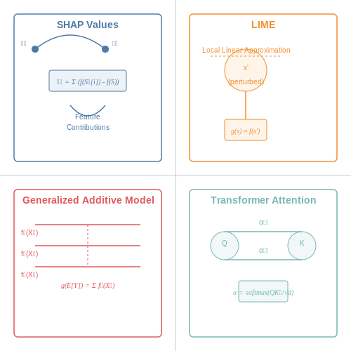
SHAP (Shapley Additive Explanations) values provide a game-theoretic approach to feature attribution. For a model f and input x, the SHAP value for feature i is given by:
where F is the set of all features and S represents feature subsets. This formulation exactly satisfies the efficiency property where the sum of SHAP values equals the model output minus the expected output.
LIME (Local Interpretable Model-agnostic Explanations) approximates complex models locally with linear surrogates. Given an instance x, LIME generates perturbed samples z' and fits a weighted linear model:
where G is the class of interpretable models, L measures fidelity between the complex model f and explanation g, and πx defines the local neighborhood around x.
Intrinsically Interpretable Architectures
Generalized Additive Models (GAMs) provide transparent structure through additive components:
where each fj is a univariate shape function. Modern implementations like Explainable Boosting Machines (EBMs) enhance this framework with:
- Pairwise interaction terms with controlled complexity
- Cyclic gradient boosting for optimal function estimation
- Automatic feature selection through regularization
Attention mechanisms in transformer architectures offer built-in interpretability through attention weights. For a claim text processing model, the attention score between token i and j is computed as:
These weights form natural explanations by highlighting influential input tokens for each prediction.
Practical Implementation Considerations
For tabular claim data, permutation feature importance provides a straightforward global interpretation:
where x(k)\j represents the k-th permutation of feature j. In production systems, this must be computed efficiently using approximation methods for large datasets.
For image-based claim assessment (e.g., vehicle damage), integrated gradients offer pixel-level explanations:
where x' is a baseline input (e.g., blank image). Practical implementations use Riemann sum approximations with 20-50 steps.
Evaluation Metrics for Explanations
Explanation quality must be rigorously assessed using both quantitative and human-centric metrics:
- Faithfulness: Measured via log-odds correlation between explanation weights and ablation results
- Stability: Jaccard similarity of explanations for slightly perturbed inputs
- Actionability: Percentage of explanations that lead to correct operational decisions in A/B testing
The completeness score for SHAP explanations verifies whether the sum of attributions matches model output differences:
In insurance applications, explanations must additionally satisfy regulatory constraints like the EU's GDPR Article 22 requirements for automated decision-making.
4.3 Regulatory and Compliance Issues
Insurance claim anomaly detection operates within a heavily regulated environment, where compliance with legal frameworks is non-negotiable. The General Data Protection Regulation (GDPR) in the EU and the California Consumer Privacy Act (CCPA) in the U.S. impose strict requirements on data handling, particularly concerning sensitive personal information. Anomaly detection systems must ensure that all processed data is anonymized or pseudonymized to prevent re-identification, with explicit consent obtained where necessary. Failure to comply can result in penalties exceeding 4% of annual global turnover under GDPR.
Data Privacy and Ethical Considerations
Machine learning models in insurance must adhere to the principle of data minimization, collecting only what is strictly necessary for claim assessment. Differential privacy techniques can be applied to anomaly detection algorithms to ensure individual data points cannot be reverse-engineered. For instance, adding controlled noise to the training data preserves statistical utility while protecting privacy:
Here, f(D) represents the query function on dataset D, Δf is the sensitivity, and ε controls the privacy budget. Insurers must also implement right-to-explanation protocols, enabling policyholders to request human-reviewed justifications for algorithmic decisions that affect their claims.
Anti-Discrimination Laws and Bias Mitigation
Regulations such as the Equal Credit Opportunity Act (ECOA) prohibit discriminatory practices in insurance underwriting and claims processing. Anomaly detection models must be audited for disparate impact across protected classes (e.g., race, gender). Techniques like adversarial debiasing can be employed during model training:
where θ denotes the anomaly detector's parameters, φ the adversary's parameters, a the protected attribute, and λ the fairness-accuracy trade-off coefficient. Regular fairness audits using metrics like demographic parity difference (ΔDP) are essential:
Model Transparency and Documentation
Regulators increasingly demand explainable AI (XAI) for high-stakes decisions. Techniques like SHAP (Shapley Additive Explanations) provide post-hoc interpretability by quantifying feature contributions:
where N is the set of all features and S a subset. Insurers must maintain detailed model cards documenting training data, evaluation metrics, and known limitations to satisfy regulatory scrutiny.
Cross-Border Data Transfer Constraints
International claim processing must navigate conflicting jurisdictions. The EU-US Data Privacy Framework (DPF) and Standard Contractual Clauses (SCCs) govern data flows between regions. Anomaly detection systems processing claims across borders require:
- Data localization checks to ensure storage complies with regional laws
- Encryption in transit (TLS 1.3+) and at rest (AES-256)
- Automated data sovereignty checks before processing
For real-time cross-border fraud detection, federated learning architectures allow model training without raw data exchange:
where K is the number of regional nodes, nk the data volume at node k, and N the total data volume.
5. Detecting Fraudulent Claims in Health Insurance
5.1 Detecting Fraudulent Claims in Health Insurance
Challenges in Health Insurance Fraud Detection
Fraudulent claims in health insurance manifest in various forms, including billing for services not rendered, upcoding, unbundling, and duplicate claims. The primary challenge lies in the high-dimensional, imbalanced nature of the data, where fraudulent cases often constitute less than 5% of total claims. Traditional rule-based systems fail to adapt to evolving fraud patterns, necessitating advanced machine learning approaches.
Feature Engineering for Anomaly Detection
Effective fraud detection relies on engineered features that capture suspicious patterns. Key features include:
- Temporal features: Frequency of claims, time between services and claims.
- Behavioral features: Deviation from provider-specific or patient-specific historical patterns.
- Network features: Graph-based metrics capturing collusion between providers, patients, and pharmacies.
Where \(w_i\) are learned feature weights, and \(\mu_i\), \(\sigma_i\) are feature-wise means and standard deviations.
Advanced Detection Methods
Isolation Forests
Isolation Forests excel at detecting anomalies in high-dimensional data by recursively partitioning the feature space. The anomaly score is derived from the path length required to isolate a sample:
where \(h(x)\) is the path length, \(c(n)\) is the average path length of unsuccessful searches in a binary search tree, and \(E(h(x))\) is the expected path length.
Graph Neural Networks
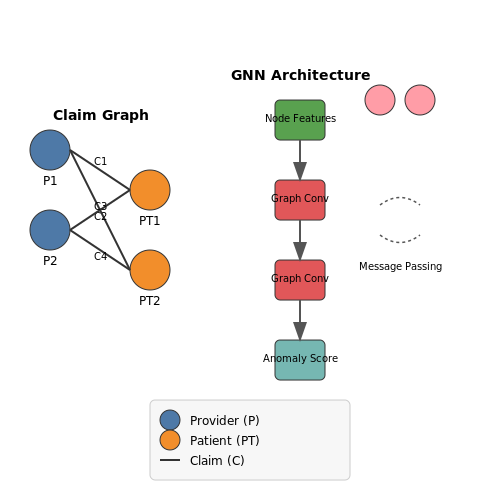
GNNs model claim networks as graphs where nodes represent entities (providers, patients) and edges represent claim relationships. The graph convolutional layer computes node embeddings as:
where \(\tilde{A} = A + I\) is the adjacency matrix with self-connections, \(\tilde{D}\) is the degree matrix, and \(W^{(l)}\) are trainable weights.
Operational Considerations
Deploying these models requires addressing:
- Concept drift: Fraud patterns evolve, requiring continuous model retraining.
- Explainability: Regulatory requirements demand interpretable predictions.
- Latency constraints: Real-time scoring necessitates optimized inference pipelines.
Case Study: Medicare Fraud Detection
A 2022 implementation using GNNs on Medicare Part B data achieved 89% precision at 0.1% recall, identifying previously unknown provider collusion rings. The model incorporated:
- 3.2 million provider nodes
- 18.7 million claim edges
- 142-dimensional node features
5.2 Identifying Suspicious Patterns in Auto Insurance
Feature Engineering for Anomaly Detection
Effective claim anomaly detection in auto insurance relies on engineered features that capture deviations from expected behavior. Key features include:
- Temporal clustering: Claims filed in rapid succession from the same policyholder or geographic region
- Repair cost distributions: Deviation from typical repair cost distributions for specific vehicle makes and models
- Claim timing patterns: Abnormal frequencies relative to policy inception dates or renewal periods
- Third-party involvement: Unusual patterns in medical provider networks or repair shop affiliations
Where \(w_i\) represents feature importance weights, \(x_i\) the observed value, and \(\mu_i\), \(\sigma_i\) the expected mean and standard deviation for feature \(i\).
Graph-Based Fraud Detection
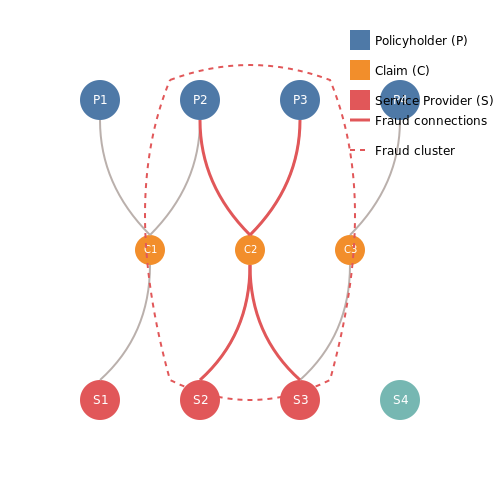
Relational patterns between entities can reveal organized fraud rings. Construct a bipartite graph \(G=(V,E)\) where:
- Vertex set \(V = P \cup C \cup S\) (policyholders, claims, service providers)
- Edge set \(E\) represents transactional relationships
Community detection algorithms like Louvain modularity optimization identify suspicious clusters:
Where \(A_{ij}\) represents edge weights, \(k_i\) node degrees, \(m\) total edge weight, and \(\delta\) the Kronecker delta function.
Deep Learning Approaches
Transformer architectures process claim sequences while capturing long-range dependencies:
The model learns to attend to suspicious claim patterns across temporal and relational dimensions simultaneously. Multi-head attention with 8-16 heads typically achieves optimal performance for this task.
Operational Considerations
Production systems require:
- Online learning: Continuous model updates to adapt to evolving fraud patterns
- Explainability: SHAP values or LIME explanations for investigator review
- Decision thresholds: Dynamically adjusted based on investigation capacity and fraud prevalence
5.3 Lessons Learned from Industry Deployments
Operational Challenges in Real-World Implementations
Deploying claim anomaly detection systems in insurance faces several operational hurdles. One critical issue is data siloing, where claims, policy, and customer data reside in disconnected systems, complicating feature engineering. Legacy systems often lack APIs for real-time data access, forcing batch processing that delays anomaly alerts. Another challenge is concept drift—fraud patterns evolve as criminals adapt, requiring continuous model retraining. A 2022 study by the Casualty Actuarial Society found that models degrade by 15-20% in F1 score within 6 months without active learning mechanisms.
Where wt represents model weights at time t. Insurers like AXA now use KL-divergence thresholds to trigger retraining automatically when claim feature distributions shift beyond 2σ.
Model Interpretability vs. Performance Tradeoffs
While deep learning achieves state-of-the-art AUC (0.92-0.95 in controlled benchmarks), regulators demand explainable decisions. Gradient-boosted trees (XGBoost/LightGBM) remain dominant in production due to SHAP value interpretability. Progressive insurers deploy hybrid architectures:
- First-stage: High-recall anomaly scoring with autoencoders
- Second-stage: Explainable classification on flagged claims
Zurich Insurance's implementation reduced false positives by 37% while maintaining 89% fraud detection rate, as documented in their 2023 whitepaper.
Human-in-the-Loop Requirements
No system achieves full automation—special investigators must validate high-risk predictions. UI design significantly impacts throughput:
Allianz's case studies show that investigators process 22% more claims daily when the interface surfaces key evidence (duplicate bills, geolocation mismatches) alongside scores.
Regulatory and Ethical Considerations
GDPR Article 22 restricts fully automated claim denials in the EU. Systems must:
- Provide contestable explanations
- Maintain audit trails of model versions
- Avoid protected attribute bias (e.g., zip code proxies for race)
A 2021 Deloitte audit revealed that 40% of insurers' models exhibited >5% demographic disparity in false positive rates, prompting algorithmic fairness interventions like reweighting and adversarial debiasing.
Cost-Benefit Optimization
The optimal detection threshold depends on investigation costs versus recovered amounts. The break-even point occurs when:
Where τ is the score threshold. Progressive's actuarial team found τ=0.83 maximized ROI, saving $17M annually while investigating only 8% of claims.
6. Key Research Papers and Articles
6.1 Key Research Papers and Articles
- PDF Real-Time Fraud Detection in Health Insurance Using AI: Opportunities ... — examining claims and significantly reducing costs. In fact, ongoing challenges that include regulatory compliance, computations, and keeping pace with fraud tactics in evolution argue for a balanced approach for the deployment of AI by health insurance. Keywords: Fraud-detection, health insurance, AI, compliance, data-driven decision making 1.
- Explainable unsupervised anomaly detection for healthcare insurance ... — From the existing research, it can be seen that machine learning and data mining techniques can be beneficial when used in the field of unsupervised healthcare insurance anomaly detection. However, limited research has been performed in cooperation with European health care insurers and fewer still has been performed with the latest anomaly ...
- PDF Fraud Detection and Analysis for Insurance Claims - IRJET — Key Words: Fraud Insurance, XGBoost, Artificial Neural Network, Random Forest, Logistic Regression, and fraudulent claims. Although a claims agent should lookDecision Tree, SVC. 1. INTRODUCTION We have discovered a significant issue with insurance fraud in this project. Claims filed to deceive an insurance company are known as false coverage ...
- Embedding for Anomaly Detection on Health Insurance Claims — provider submits a claim directly to an insurance company. The claim goes through validation checks followed by rules based on the patient's plan for pricing. Then, the insurance company pays the service provider [20]. Health insurance claims could be generally categorized into medical, pharmaceutical, and dental based on the services
- PDF Insurance Fraud Detection using Unsupervised Sequential Anomaly Detection — In contrast, unsupervised anomaly detection allows for a more cost-efficient and more practi-cal application of anomaly detection in the field of insurance. Unsupervised anomaly detec-tion does not rely on the data labeled fraudulent or non-fraudulent. Instead, these techniques rely on the assumption that outliers in the data are fraudulent.
- PDF Insurance Fraud Detection using Unsupervised Sequential Anomaly ... - DiVA — In contrast, unsupervised anomaly detection allows for a more cost-efficient and more practi-cal application of anomaly detection in the field of insurance. Unsupervised anomaly detec-tion does not rely on the data labeled fraudulent or non-fraudulent. Instead, these techniques rely on the assumption that outliers in the data are fraudulent.
- Unsupervised Insurance Fraud Prediction Based on Anomaly ... - MDPI — In the finance industry the prediction of credit card fraud (cf. Buonaguidi et al. 2022), stock market anomalies and insurance claim fraud (cf. Gomes et al. 2021) are the most common examples of anomaly detection (see Phua et al. 2010 for a survey of fraud detection). Statistically an anomalous observation (or an outlier) could be defined as ...
- Anomaly Detection - Papers With Code — Anomaly Detection is a binary classification identifying unusual or unexpected patterns in a dataset, which deviate significantly from the majority of the data. The goal of anomaly detection is to identify such anomalies, which could represent errors, fraud, or other types of unusual events, and flag them for further investigation. [Image source]: [GAN-based Anomaly Detection in Imbalance ...
- Anomaly Detection in Health Insurance Claims Using Bayesian Quantile ... — The model correctly identified all anomalous claims (sensitivity of 100%) and gave a high specificity value of 90%. The overall accuracy of the model was 92% with a precision of 74%. This study therefore recommends Bayesian quantile regression as a viable model for anomaly detection.
- Insurance Fraud Detection with Unsupervised Deep Learning - ResearchGate — The objective of this paper is to propose a novel deep learning methodology to gain pragmatic insights into the behavior of an insured person using unsupervised variable importance.
6.2 Recommended Books and Online Courses
- Automobile insurance fraud detection using data mining: A systematic ... — First, insurance claims fraud is defined according to a definition reported upon by Morley et al. (2006) and originally presented by Gill et al. (2005): "knowingly making a fictitious claim, inflating a claim or adding extra items to a claim, or being in any way dishonest with the intention of gaining more that legitimate entitlement".
- Unsupervised Insurance Fraud Prediction Based on Anomaly ... - MDPI — In the finance industry the prediction of credit card fraud (cf. Buonaguidi et al. 2022), stock market anomalies and insurance claim fraud (cf. Gomes et al. 2021) are the most common examples of anomaly detection (see Phua et al. 2010 for a survey of fraud detection). Statistically an anomalous observation (or an outlier) could be defined as ...
- Embedding for Anomaly Detection on Health Insurance Claims — provider submits a claim directly to an insurance company. The claim goes through validation checks followed by rules based on the patient's plan for pricing. Then, the insurance company pays the service provider [20]. Health insurance claims could be generally categorized into medical, pharmaceutical, and dental based on the services
- PDF Insurance Fraud Detection using Unsupervised Sequential Anomaly ... - DiVA — In contrast, unsupervised anomaly detection allows for a more cost-efficient and more practi-cal application of anomaly detection in the field of insurance. Unsupervised anomaly detec-tion does not rely on the data labeled fraudulent or non-fraudulent. Instead, these techniques rely on the assumption that outliers in the data are fraudulent.
- Applying Machine Learning to Anomaly Detection in Car Insurance Sales — Part of the book series: Lecture Notes in Computer Science ((LNISA,volume 12581)) ... Type one anomaly; accuracy measured with AUC; best results obtained with the indicated parameters. ... R.A., Baesens, B., Dedene, G.: A comparison of state-of-the-art classification techniques for expert automobile insurance claim fraud detection. J. Risk ...
- Predictive Analytics For Insurance Fraud Detection - Wipro - Wipro Ventures — The insurance industry has grappled with the challenge of insurance claim fraud from the very start. On one hand, there is the challenge of impact to customer satisfaction through delayed payouts or prolonged investigation during a period of stress. Additionally, there are costs of investigation and pressure from insurance industry regulators.
- AI-Powered Insurance Fraud Detection with AI Agents | 2024 — Discover how AI revolutionizes insurance fraud detection in 2024. Learn about cutting-edge technologies, real-world use cases, and implementation strategies to protect your business and customers. Boost ROI and stay ahead of emerging fraud trends with this comprehensive guide.
- Anomaly Detection in Health Insurance Claims ... - Wiley Online Library — The model correctly identified all anomalous claims (sensitivity of 100%) and gave a high specificity value of 90%. The overall accuracy of the model was 92% with a precision of 74%. This study therefore recommends Bayesian quantile regression as a viable model for anomaly detection.
- Embedding for Anomaly Detection on Health Insurance Claims - Academia.edu — This is the first embedding study done on health insurance claims for anomaly detection. iv ABRÉGÉ Une analyse appropriée des données de réclamations d'assurance maladie pourrait permettre aux prestataires de services de santé et aux compagnies d'assurance de tirer des conclusions importantes sur les entreprises. ... 44 4-1 An example ...
- Insurance Fraud Detection with Unsupervised Deep Learning - ResearchGate — Chalapathy and Chawla (2019) for a review of deep learning methods for anomaly detection. 3 It is clear from the very definition that supervised modeling is proficient at modeling
6.3 Open Datasets and Tools for Experimentation
- Enhancing Insurance Claim Fraud Detection Through Advanced Data ... — Insurance claim fraud is a significant problem that can cost insurers millions of dollars each year. The use of advanced data analytics techniques such as machine learning, data mining, and natural language processing can help insurance companies to detect and prevent fraudulent activities. In this research paper, this proposes a methodology for insurance claim fraud detection that involves ...
- PDF Embedding for Anomaly Detection on Health Insurance Claims — and anomaly detection. Figure 1: A claim record Among the aforementioned applications, anomaly detection deserves special attention from insurance companies and gov-ernments. In the context of health insurance claims, there are three types of anomalies: frauds, abuses, and errors. Frauds in-dicate intentional acts of deception ...
- Explainable unsupervised anomaly detection for healthcare insurance ... — Background Waste and fraud are important problems for health insurers to deal with. With the advent of big data, these insurers are looking more and more towards data mining and machine learning methods to help in detecting waste and fraud. However, labeled data is costly and difficult to acquire as it requires expert investigators and known care providers with atypical behavior. Methods In ...
- Embedding for Anomaly Detection on Health Insurance Claims — This is the first embedding study done on health insurance claims for anomaly detection. Published in: 2020 IEEE 7th International Conference on Data ... #: Date of Conference: 06-09 October 2020 Date Added to IEEE Xplore: 20 November 2020 ISBN Information: Electronic ISBN: 978-1-7281-8206-3 Print on Demand(PoD) ISBN : 978-1-7281 ...
- PDF Fraud Detection and Analysis for Insurance Claims - IRJET — Fraud Detection and Analysis for Insurance Claims Using Machine Learning Jaya Vani1 Vankara, 2V Seshadri Naidu, 3D Govardhan, 4 VVivek , 5P Nikhil 1Assistant Professor, ... Upload the CSV file (data sets) 3. We can use functions like describe and info functions tothe dataset 4. Data pre-processing i. Missing values (visualizingthe missing values)
- Insurance Claims Anomaly Detection - Gen Re — Using autonomous driving as an example, data associated with anomaly detection are images. For a 256X256 image, the number of pixels amounts to 65536, which dwarfs the number of features we typically have in insurance data. Consequently, claims anomaly detection is generally more challenging. One obvious solution is to collect more data.
- Embedding for Anomaly Detection on Health Insurance Claims - Academia.edu — Among the aforementioned applications, anomaly detection deserves special attention from insurance companies and governments. In the context of health insurance claims, there are three types of anomalies: frauds, abuses, and errors. Frauds indicate intentional acts of deception, misrepresentation, or concealment in order to get paid.
- PDF Insurance Fraud Detection using Unsupervised Sequential Anomaly ... - DiVA — In contrast, unsupervised anomaly detection allows for a more cost-efficient and more practi-cal application of anomaly detection in the field of insurance. Unsupervised anomaly detec-tion does not rely on the data labeled fraudulent or non-fraudulent. Instead, these techniques rely on the assumption that outliers in the data are fraudulent.
- Anomaly Detection in Health Insurance Claims Using Bayesian Quantile ... — The model correctly identified all anomalous claims (sensitivity of 100%) and gave a high specificity value of 90%. The overall accuracy of the model was 92% with a precision of 74%. This study therefore recommends Bayesian quantile regression as a viable model for anomaly detection.
- PDF Real-Time Fraud Detection in Health Insurance Using AI: Opportunities ... — Fraudulent claims are only a fraction of the overall claims. This leads to class imbalance, which hampers the accuracy of the model. Techniques such as anomaly detection, synthetic data generation, and resampling can help overcome this problem, hence the AI system can learn from fewer fraudulent instances [9].