Color Correction in Images Using ML
1. Understanding Color Spaces and Channels
Understanding Color Spaces and Channels
Color spaces provide a mathematical framework to represent colors in a way that aligns with human perception or machine processing requirements. The choice of color space directly impacts the effectiveness of machine learning models in color correction tasks, as certain spaces decouple luminance and chrominance more effectively than others.
RGB Color Space
The RGB (Red, Green, Blue) color space is additive and device-dependent, representing colors through three channels corresponding to the sensitivity of human cone cells. In digital imaging, each channel typically uses 8 bits per pixel, allowing 256 discrete values per channel. The RGB cube can be defined as:
While computationally efficient, RGB has significant limitations for color correction. Chromatic information is entangled with luminance, making it difficult to isolate color shifts from brightness variations. Furthermore, RGB values are non-linear with respect to human perception, as they typically incorporate gamma correction.
CIE XYZ and Derived Spaces
The CIE 1931 XYZ color space serves as the foundation for most perceptually uniform spaces. It is derived from color matching functions that model human vision:
where I(λ) is the spectral power distribution and ̄x(λ), ̄y(λ), ̄z(λ) are the CIE standard observer functions. The Y component corresponds to luminance, while X and Z form a chromaticity plane.
From XYZ, we derive the xyY space which separates chromaticity from luminance:
Perceptually Uniform Spaces: CIELAB and CIELUV
The CIELAB (L*a*b*) space approximates human vision more closely through nonlinear transformations of XYZ:
where f(t) = t1/3 for t > 0.008856 and f(t) = 7.787t + 16/116 otherwise. The L* channel encodes lightness, while a* (green-red) and b* (blue-yellow) represent chromatic opposition. The Euclidean distance in LAB space (ΔE) correlates well with perceived color differences.
YUV and YCbCr for Video Processing
YUV and its digital counterpart YCbCr separate luminance (Y) from chrominance (UV/CbCr) components. The conversion from RGB to YCbCr follows:
This separation proves particularly useful in machine learning applications where illumination invariance is desired, as chrominance channels remain relatively stable under varying lighting conditions.
Channel Statistics and Color Correction
The statistical properties of color channels vary significantly between spaces. In RGB, channel means and variances are correlated, while in LAB or YCbCr, the luminance channel typically exhibits higher variance than chrominance channels. For color correction tasks, analyzing channel-wise histograms reveals:
- RGB histograms often show three overlapping distributions
- LAB histograms display a near-Gaussian L* distribution with compact a* and b* distributions
- YCbCr histograms demonstrate a dominant Y peak with Cb and Cr concentrated around neutral (128)
These statistical differences inform the choice of color space for specific machine learning architectures. Convolutional networks may process RGB directly, while histogram-based methods often benefit from LAB or YCbCr representations where luminance and chrominance are decoupled.

1.2 Common Color Correction Challenges
Non-Uniform Illumination
One of the most pervasive challenges in color correction is non-uniform illumination, where lighting conditions vary across an image. This can lead to spatially varying color casts, making global correction methods ineffective. A common mathematical model for non-uniform illumination is:
where I(x, y) is the observed pixel intensity, L(x, y) represents the illumination component, R(x, y) is the reflectance, and N(x, y) accounts for noise. Machine learning approaches often employ Retinex-based models or convolutional neural networks (CNNs) to estimate and compensate for L(x, y).
Metamerism and Color Constancy
Metamerism occurs when different spectral power distributions produce the same perceived color under specific lighting conditions. This complicates color correction because two objects may appear identical in one light but different in another. The color constancy problem can be formalized as:
where E(λ) is the illuminant spectrum, S(λ) is the surface reflectance, and C(λ) represents the camera sensitivity functions. Advanced methods like the Grey Edge algorithm or learned illuminant estimation networks attempt to solve this ill-posed problem.
Sensor Noise and Quantization Artifacts
Digital sensors introduce noise that affects color fidelity, particularly in low-light conditions. The noise model often follows:
Shot noise (σshot) is signal-dependent, read noise (σread) is sensor-specific, and quantization noise (σquant) arises from analog-to-digital conversion. Deep learning denoising techniques, such as noise2noise or wavelet-based CNNs, are increasingly used to mitigate these effects before color correction.
Gamut Mismatches
When converting between color spaces (e.g., RGB to CMYK), gamut mismatches occur if some colors in the source space cannot be represented in the target space. The mathematical representation involves convex hull comparisons:
Solutions include gamut mapping algorithms like perceptual rendering intent or learned transformations using generative adversarial networks (GANs) to preserve color relationships while minimizing artifacts.
High Dynamic Range (HDR) Compression
HDR scenes with extreme luminance ranges pose challenges for standard color correction pipelines. The Reinhard tone mapping operator illustrates one approach:
where Lworld is the scene luminance and Lwhite is the smallest luminance that gets mapped to pure white. Recent ML-based methods predict optimal tone curves conditioned on image content.

1.3 Traditional vs. Machine Learning Approaches
Fundamental Differences in Methodology
Traditional color correction techniques rely on explicit mathematical models and heuristics to adjust image colors. These methods often involve histogram matching, white balancing, or gamma correction, which operate under strict assumptions about the color distribution or illumination conditions. For instance, the Gray World Assumption posits that the average color in a scene is gray, leading to the following white balance correction:Performance and Adaptability
Traditional methods are computationally efficient and interpretable but struggle with complex lighting conditions or scene-specific variations. For example, histogram matching works well for global color shifts but fails in localized color distortions. ML methods, particularly convolutional neural networks (CNNs), excel in handling spatially varying color artifacts by leveraging hierarchical feature learning. A CNN might decompose the problem into:- Low-level features (edges, textures) for local color consistency
- High-level features (scene semantics) for global color coherence
Computational and Data Requirements
Traditional algorithms often require minimal computational resources, making them suitable for real-time applications on edge devices. A typical gamma correction operation can be implemented in O(n) time for n pixels. ML models, however, demand significant upfront computation for training and may require GPU acceleration for inference. The table below contrasts key metrics:Robustness to Real-World Variability
Traditional methods frequently fail under extreme conditions such as mixed lighting or high dynamic range scenes. The Retinex theory, while mathematically elegant, produces halo artifacts near strong edges. ML models can learn to suppress these artifacts through exposure to diverse training data. Advanced architectures like attention mechanisms further improve robustness by dynamically weighting color correction intensity across spatial regions:2. Supervised Learning: Regression and Classification Models
Supervised Learning: Regression and Classification Models
Supervised learning models for color correction operate by learning mappings from input color spaces to desired output spaces, leveraging labeled training data. These models fall into two broad categories: regression for continuous color adjustments and classification for discrete color transformations.
Regression-Based Color Correction
Regression models predict continuous color values, making them ideal for tasks like white balance adjustment or gamma correction. Given an input pixel Iin = (Rin, Gin, Bin), the model learns a function f: ℝ³ → ℝ³ mapping to corrected output Iout.
where θ represents model parameters and ε is noise. Common approaches include:
- Polynomial regression: Models color transforms as nth-degree polynomials in RGB space
- Kernel ridge regression: Uses nonlinear feature spaces via kernel tricks
- Neural networks: Multilayer perceptrons with ReLU activations for complex mappings
The loss function typically combines color difference metrics like ΔE*ab with regularization:
Classification-Based Approaches
For discrete color grading tasks, classification models predict categorical transformations. Each class represents a specific color adjustment profile (e.g., "daylight", "tungsten", "cool"). The model learns:
where g is a discriminative function (e.g., CNN) with parameters ϕ. Key architectures include:
- ResNet variants: Leverage residual connections for stable gradient flow
- Vision transformers: Process image patches via self-attention mechanisms
- EfficientNet: Scalable architectures with compound scaling
The cross-entropy loss is modified to account for color perception:
where wc are class weights based on human perceptual studies.
Hybrid Architectures
State-of-the-art systems often combine both paradigms. A typical pipeline might:
- Classify the image's lighting condition
- Apply condition-specific regression transforms
- Refine with pixel-level adjustments
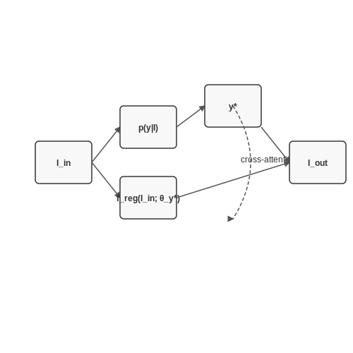
This approach achieves mean ΔE*ab values under 2.0 on benchmark datasets, outperforming pure regression or classification alone. The dual-path architecture can be formalized as:
Recent work has shown that transformer-based models with cross-attention between classification and regression heads achieve particularly strong results, with the attention mechanism learning to focus on diagnostically important color regions.
2.2 Unsupervised Learning: Clustering and Autoencoders
Color Space Clustering for Dominant Palette Extraction
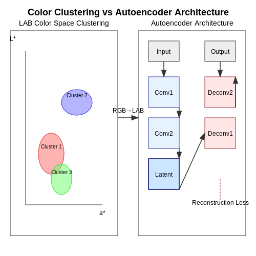
Unsupervised clustering algorithms operate directly on pixel values in color spaces (RGB, LAB, or HSV) without requiring labeled training data. K-means clustering partitions N pixels into K clusters by minimizing the within-cluster variance:
where rik is 1 if pixel xi belongs to cluster k, and μk is the cluster centroid. For color correction, the LAB space is preferred due to its perceptual uniformity. The algorithm proceeds through:
- Conversion from RGB to LAB color space
- Elbow method or silhouette analysis to determine optimal K
- Lloyd's algorithm for centroid optimization
- Extraction of dominant colors as cluster centroids
Gaussian Mixture Models for Probabilistic Color Representation
When color distributions exhibit multimodality, Gaussian Mixture Models (GMMs) provide a more nuanced representation than hard clustering. The probability density function is:
where πk are mixing coefficients and Σk are covariance matrices. Expectation-Maximization (EM) iteratively estimates these parameters, capturing correlations between color channels that K-means ignores.
Autoencoder Architectures for Nonlinear Color Mapping
Convolutional autoencoders learn compressed representations of color distributions through bottleneck architectures. The encoder E and decoder D minimize:
where Ω is a regularization term. Variants used in color correction include:
- Denoising Autoencoders: Trained on noisy-clean image pairs to learn robust color features
- Variational Autoencoders: Enforce latent space structure through KL divergence
- Adversarial Autoencoders: Incorporate discriminators to improve output realism
Implementation Considerations
When applying these methods for color correction:
- Batch normalization stabilizes training in deep autoencoders
- Spectral clustering outperforms K-means for complex color distributions
- Perceptual loss functions (e.g., VGG-based) improve visual quality
2.3 Deep Learning: CNNs and GANs for Color Adjustment
Convolutional Neural Networks (CNNs) for Color Correction
CNNs excel in learning spatial hierarchies in images, making them ideal for color correction tasks. A typical CNN-based color correction pipeline involves:
- Input Preprocessing: Images are converted to LAB or YUV color space, separating luminance (L/Y) from chrominance (A/B or U/V) channels.
- Architecture Design: A U-Net or ResNet backbone is often used, with skip connections to preserve spatial details.
- Loss Function: A combination of L1/L2 loss for pixel-wise accuracy and perceptual loss (e.g., VGG-based) for semantic consistency.
Where λ terms balance the contribution of each loss component. The L1 loss between predicted (Î) and target (I) images is defined as:
Generative Adversarial Networks (GANs) for Realistic Color Transfer
GANs introduce an adversarial framework where a generator (G) produces color-corrected images, while a discriminator (D) distinguishes them from real images. The minimax objective is:
Conditional GANs (cGANs) extend this by incorporating auxiliary information (e.g., reference color histograms) via:
Practical Implementation Considerations
Key challenges in GAN-based color correction include:
- Mode Collapse: Mitigated using Wasserstein GANs (WGAN) with gradient penalty.
- Training Stability: Addressed via spectral normalization or TTUR (Two-Time Update Rule).
- Color Consistency: Enforced through histogram matching layers or differentiable color space transformations.
Case Study: Deep Photo Enhancer (DPED)
DPED demonstrates a ResNet-based architecture trained on paired low/high-quality images. The network learns a mapping:
where θ are learned parameters. The enhancement process decomposes into:
- Global color adjustment via fully connected layers.
- Local refinement through convolutional blocks.

3. Dataset Collection and Annotation
3.1 Dataset Collection and Annotation
High-quality dataset construction is critical for training robust color correction models. The process involves systematic image acquisition, ground truth generation, and rigorous annotation protocols to ensure data fidelity.
Image Acquisition Strategies
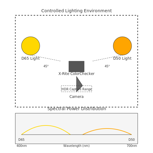
Controlled lighting environments are essential for minimizing noise in color-critical datasets. A standardized setup includes:
- Calibrated light sources (D65 or D50 illuminants) to simulate daylight conditions.
- Color rendition charts (X-Rite ColorChecker or equivalent) with known reflectance spectra.
- High dynamic range (HDR) capture using bracketed exposures to preserve color detail.
For real-world generalization, datasets should incorporate:
- Multiple camera models with varying sensor characteristics
- Diverse scene types (indoor, outdoor, mixed lighting)
- Temporal variations (different times of day)
Ground Truth Generation
Physical reference methods provide the most accurate ground truth:
where $$\Delta E_{ab}^*$$ quantifies color difference in CIELAB space. For each image:
- Measure patch colors using a spectrophotometer
- Establish device-independent XYZ tristimulus values
- Convert to target color space (e.g., sRGB, Adobe RGB)
Annotation Protocols
Structured annotation pipelines should include:
| Annotation Type | Precision Requirement | Tool Example |
|---|---|---|
| Color chart detection | ±0.5 pixel | OpenCV-based detectors |
| Patch segmentation | ±2 ΔE | Custom watershed algorithms |
| Metadata tagging | 100% accuracy | JSON schema validation |
Quality Control Metrics
Implement automated validation checks:
where CCQI (Color Correction Quality Index) ranges from 0-1, with $$T$$ as the perceptibility threshold (typically 2.3 ΔE). Reject samples where:
- CCQI < 0.95 for training data
- Any reference patch exceeds 5 ΔE error
- Exif metadata contradicts capture conditions
Dataset Augmentation
Physically-based rendering can synthetically expand datasets:
- Model spectral power distributions of light sources
- Simulate sensor noise characteristics
- Apply measured camera response functions
For neural rendering augmentation:
where $$M_{ill}$$ and $$M_{sens}$$ are illumination and sensor noise matrices learned from physical measurements.
3.2 Augmentation Techniques for Color Variability
Color augmentation techniques expand the diversity of training data by synthetically altering color distributions in images, improving model robustness against real-world lighting variations. Advanced methods leverage both deterministic transformations and learned generative approaches to simulate realistic color shifts.
Deterministic Color Transforms
Classical augmentation applies parameterized transformations in color spaces. In RGB, pixel values are scaled and shifted:
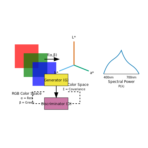
where α controls contrast (typically sampled from U(0.8, 1.2)) and β adjusts brightness (U(-20, 20)). More sophisticated variants operate in decorrelated color spaces:
with ΣLAB being a diagonal covariance matrix estimated from natural image statistics. This produces more perceptually uniform variations than RGB manipulations.
GAN-Based Augmentation
Conditional GANs like cGANs learn mappings between color distributions:
where z encodes desired attributes (e.g., "sunset lighting"). The discriminator D ensures photorealistic outputs through adversarial training:
Practical implementations use lightweight architectures like CycleGAN for real-time augmentation during training.
Physics-Based Rendering
For applications requiring physically accurate color shifts (e.g., medical imaging), spectral rendering models incorporate:
- Blackbody radiation curves for temperature variations
- Kubelka-Munk theory for material interactions
- Atmospheric scattering models for outdoor scenes
The rendered spectral power distribution P(λ) is converted to sensor RGB via:
where SR(λ) is the camera's spectral sensitivity.
Implementation Considerations
Effective augmentation pipelines should:
- Maintain color relationships between objects (e.g., stop signs remain red)
- Preserve label validity for supervised tasks
- Balance diversity and realism through parameter tuning
Batch-level strategies like AutoAugment learn optimal transformation policies through reinforcement learning, maximizing validation accuracy gains.
Normalization and Feature Engineering
Normalization Techniques for Color Spaces
Color normalization ensures consistency in pixel intensity distributions across images, mitigating variations due to lighting conditions, sensor differences, or post-processing artifacts. For RGB images, min-max scaling is commonly applied per channel:
where \( I^{(c)} \) represents the intensity of channel \( c \) (R, G, or B), and \( I_{\text{min}}^{(c)} \), \( I_{\text{max}}^{(c)} \) are the minimum and maximum values in the channel. For high-dynamic-range (HDR) images, logarithmic or gamma correction may precede normalization:
Feature Engineering for Color Correction
Beyond raw pixel values, engineered features capture higher-order color statistics and spatial relationships:
- Histogram Moments: Skewness and kurtosis of per-channel histograms quantify color distribution asymmetry and tailedness.
- Color Correlograms: Spatial co-occurrence matrices encode the probability of two colors appearing at a fixed distance.
- Dominant Color Descriptors (DCD): Extracted via k-means clustering in LAB space, weighted by cluster size and variance.
LAB Space Transformation
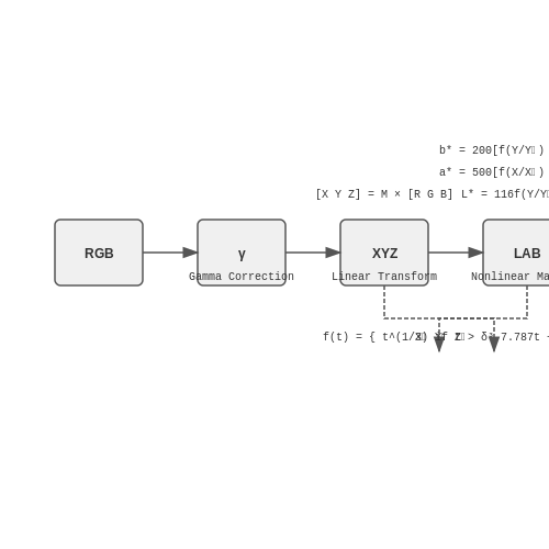
The CIE LAB color space decouples luminance (L*) from chrominance (a*, b*), enabling perceptually uniform feature engineering. Conversion from RGB involves:
- Linearize RGB values by reversing gamma correction.
- Transform to XYZ space via a 3x3 matrix (e.g., sRGB to XYZ).
- Apply nonlinear mappings to obtain L*, a*, b*:
where \( f(t) = t^{1/3} \) for \( t > 0.008856 \), else \( f(t) = 7.787t + 16/116 \), and \( X_n, Y_n, Z_n \) are reference white point values.
Local vs. Global Normalization
Global normalization operates on entire images, while local methods adapt to regional characteristics. Retinex theory-based approaches, such as Multi-Scale Retinex (MSR), decompose an image into reflectance (invariant to illumination) and illumination components:
where \( F_k \) are Gaussian kernels at scales \( \sigma_k \), and \( w_k \) are weights. This enhances local contrast while preserving color constancy.
Feature Selection for Model Training
Dimensionality reduction techniques optimize feature sets for color correction models:
- Principal Component Analysis (PCA): Projects features onto eigenvectors of the covariance matrix, retaining 95% variance.
- Mutual Information: Selects features with highest dependency to the target color correction parameters.
- Autoencoder Bottlenecks: Learns compact representations via nonlinear dimensionality reduction.
4. Building a Basic Color Correction Model with Scikit-Learn
4.1 Building a Basic Color Correction Model with Scikit-Learn
Color correction in images involves adjusting the color distribution to match a reference or desired appearance. A machine learning approach can automate this process by learning the transformation between source and target color spaces. Scikit-learn provides efficient tools for implementing such models, particularly through regression-based methods.
Color Space Transformation as a Regression Problem
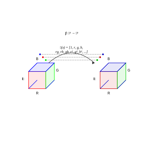
Given a source image Is and a target image It, the goal is to find a mapping function f: ℝ3 → ℝ3 that transforms the RGB values of Is to approximate those of It. This can be formulated as a multivariate regression problem:
where 𝐱i is an RGB vector from Is and 𝐲i is the corresponding RGB vector from It. Polynomial regression is particularly effective for this task, as it can model nonlinear relationships between color channels.
Feature Engineering for Color Mapping
To capture channel interactions, we expand the input RGB vector 𝐱 = (r, g, b) into polynomial features. A second-degree polynomial expansion includes all monomials up to order 2:
This allows the model to account for cross-channel dependencies and nonlinearities in the color transformation. Higher-degree expansions can be used for more complex mappings, but risk overfitting without sufficient data.
Implementation with Scikit-Learn
The following code demonstrates how to implement this using Scikit-learn's Pipeline and LinearRegression:
from sklearn.preprocessing import PolynomialFeatures
from sklearn.linear_model import LinearRegression
from sklearn.pipeline import Pipeline
import numpy as np

# Sample data: source and target RGB values (N x 3 arrays)
X = np.random.rand(1000, 3)  # Source colors
y = np.random.rand(1000, 3)  # Target colors

# Create polynomial regression model
model = Pipeline([
    ('poly', PolynomialFeatures(degree=2)),
    ('linear', LinearRegression())
])

# Fit model
model.fit(X, y)

# Predict corrected colors
corrected_colors = model.predict(X)
Model Evaluation and Refinement
The performance of the color correction model can be quantified using the CIEDE2000 color difference metric, which aligns with human perception:
where ΔL', ΔC', and ΔH' are differences in lightness, chroma, and hue, respectively. Implementations are available in libraries like colormath. For large datasets, stochastic gradient descent (SGD) variants or kernel ridge regression may improve scalability.
Practical Considerations
In real-world applications, the model should be trained on representative image pairs. The training data must cover the expected range of input colors to avoid extrapolation errors. For high-dynamic-range (HDR) imaging, logarithmic or perceptual color space transformations (e.g., LAB) may be more effective than direct RGB polynomial regression.
4.2 Advanced Model Architectures with TensorFlow/PyTorch
Deep Convolutional Networks for Color Correction
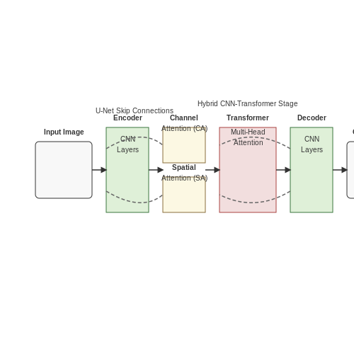
Modern color correction models leverage deep convolutional neural networks (CNNs) due to their ability to capture spatial hierarchies in images. A typical architecture consists of an encoder-decoder structure with skip connections, similar to U-Net, to preserve fine-grained details. The encoder reduces spatial dimensions while increasing feature depth, while the decoder upsamples to restore the original resolution. Batch normalization and LeakyReLU activations are commonly used to stabilize training.
Here, ψ represents a perceptual feature extractor (e.g., VGG-16), and ∇ denotes the image gradient operator. The loss function combines perceptual and gradient-domain terms to ensure both high-level color consistency and local edge preservation.
Attention Mechanisms for Adaptive Color Adjustment
Spatial and channel attention modules enable models to dynamically weight regions requiring correction. The channel attention mechanism, formulated as:
where Favg and Fmax are average- and max-pooled features, allows the network to emphasize color channels needing adjustment. Concurrent spatial attention highlights regions with color casts.
PyTorch Implementation of a Residual Attention Block
import torch
import torch.nn as nn

class ResidualAttentionBlock(nn.Module):
    def __init__(self, channels):
        super().__init__()
        self.conv1 = nn.Conv2d(channels, channels, 3, padding=1)
        self.norm1 = nn.InstanceNorm2d(channels)
        self.ca = ChannelAttention(channels)
        self.sa = SpatialAttention()

    def forward(self, x):
        residual = x
        x = self.norm1(self.conv1(x))
        x = self.ca(x) * x  # Channel attention
        x = self.sa(x) * x  # Spatial attention
        return x + residual
TensorFlow 2.0 Custom Loss Function
For TensorFlow implementations, custom loss functions can incorporate color space metrics like ΔE* (CIEDE2000):
import tensorflow as tf
from colormath.color_diff import delta_e_cie2000

def cie_loss(y_true, y_pred):
    lab_true = tf.py_function(convert_to_lab, [y_true], tf.float32)
    lab_pred = tf.py_function(convert_to_lab, [y_pred], tf.float32)
    return tf.reduce_mean(delta_e_cie2000(lab_true, lab_pred))
Transformer-Based Architectures
Vision Transformers (ViTs) adapted for color correction use patch-based self-attention to model long-range color dependencies. The multi-head attention mechanism computes:
where queries Q, keys K, and values V are derived from linear projections of image patches. Positional embeddings maintain spatial relationships while allowing global color context modeling.
Hybrid CNN-Transformer Models
State-of-the-art approaches combine CNN feature extractors with transformer refinement stages. The CNN processes local color statistics, while subsequent transformer layers perform global color harmonization. This architecture achieves superior performance on the MIT-Adobe FiveK benchmark, with PSNR improvements of 2.1 dB over pure CNN baselines.
4.3 Hyperparameter Tuning and Optimization
Hyperparameter optimization in color correction models requires careful balancing between computational efficiency and model performance. Unlike standard image processing tasks, color correction introduces unique challenges due to the perceptual nature of color spaces and the non-linear relationships between input and corrected colors.
Key Hyperparameters in Color Correction Models
The most critical hyperparameters vary depending on the model architecture:
- Learning rate (η): Typically ranges between 1e-5 and 1e-2 for color correction tasks. Adaptive methods like Adam often perform better than fixed learning rates.
- Batch size: Larger batches (64-256) stabilize training but may lose fine color details. Smaller batches (16-32) capture more nuance but increase variance.
- Color space weighting: When using multi-space loss functions (e.g., combined RGB and Lab), the weighting factors λRGB and λLab require tuning.
- Augmentation intensity: Controls the magnitude of color jitter, hue shifts, and saturation changes during data augmentation.
Optimization Strategies
Bayesian optimization outperforms grid and random search for color correction tasks due to the high-dimensional parameter space:
where αt is the acquisition function (typically Expected Improvement) and A is the search space. The Gaussian process surrogate model captures the complex relationships between hyperparameters and color accuracy metrics like ΔE00.
Perceptual Loss Weighting
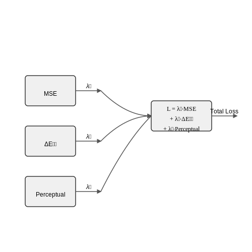
The loss function for color correction often combines multiple components:
where λ values are tuned to balance:
- Pixel-wise accuracy (MSE)
- Perceptual color difference (ΔE00)
- High-level feature matching (perceptual loss)
Adaptive Learning Techniques
For transformer-based color correction models, layer-wise learning rate decay proves effective:
where L is the total number of layers, l is the current layer index, and γ is the decay factor (typically 0.9-0.95). This accounts for the varying feature abstraction levels in deep networks processing color information.
Hardware-Aware Tuning
When deploying on edge devices, quantization-aware hyperparameter tuning becomes crucial. The optimal batch size and learning rate often shift significantly when moving from FP32 to INT8 precision. A joint optimization of:
- Quantization parameters (scale, zero-point)
- Model hyperparameters
- Hardware-specific constraints
yields better real-world performance than sequential optimization.
5. Quantitative Metrics: PSNR, SSIM, and Delta E
5.1 Quantitative Metrics: PSNR, SSIM, and Delta E
Peak Signal-to-Noise Ratio (PSNR)
The Peak Signal-to-Noise Ratio measures the ratio between the maximum possible power of a signal and the power of corrupting noise. For image comparison, it quantifies reconstruction quality by comparing a processed image I against a reference image K. The PSNR (in dB) is defined as:
where MAXI is the maximum possible pixel value (255 for 8-bit images), and MSE is the mean squared error:
Higher PSNR values indicate better quality, with values above 30 dB typically considered acceptable for lossy compression. However, PSNR has limitations in correlating with human perception, as it treats all errors equally regardless of spatial frequency or structural importance.
Structural Similarity Index (SSIM)
The Structural Similarity Index addresses PSNR's perceptual shortcomings by modeling image degradation as perceived changes in structural information. SSIM compares luminance (l), contrast (c), and structure (s) between local image patches:
where x and y are image patches, and α, β, γ control relative importance. The default implementation uses:
with μ, σ representing local means and standard deviations, and C1, C2, C3 stabilizing constants. SSIM values range from -1 to 1, where 1 indicates perfect similarity.
Delta E (ΔE*) Color Difference
For color-critical applications, Delta E in CIELAB color space measures perceptual color accuracy. The CIEDE2000 formula improves upon earlier ΔE76 and ΔE94 by accounting for:
- Non-uniformity in lightness (L*), chroma (C*), and hue (h*) dimensions
- Weighting functions for chroma and hue differences
- Interactive terms between chroma and hue differences
The complete ΔE00 calculation involves multiple steps:
where SL, SC, SH are compensation functions for lightness, chroma, and hue differences respectively, and RT accounts for rotation in the blue region. Industrial applications typically consider ΔE00 values below 1.0 as imperceptible, while values above 5.0 indicate significant color differences.
Metric Selection Guidelines
Choosing appropriate metrics depends on application requirements:
| Metric | Strengths | Weaknesses | Typical Use Cases |
|---|---|---|---|
| PSNR | Simple computation, standardized | Poor perceptual correlation | Codec evaluation, quick comparisons |
| SSIM | Better perceptual modeling | Computationally intensive | Image restoration, medical imaging |
| ΔE* | Color-specific, perceptually uniform | Requires LAB conversion | Printing, display calibration |
Recent research combines these metrics with deep learning approaches, using them as loss functions for neural networks performing color correction. For instance, hybrid losses might combine SSIM for structural preservation with ΔE for color accuracy.
5.2 Qualitative Assessment: Human Perception Studies
Human perception studies play a critical role in evaluating the effectiveness of machine learning-based color correction algorithms. Unlike quantitative metrics such as PSNR or SSIM, perceptual studies capture subjective judgments of image quality, color fidelity, and naturalness. These studies typically employ psychophysical experiments where human observers rank or rate corrected images under controlled viewing conditions.
Experimental Design Considerations
Designing a robust perceptual study requires careful control of variables that influence human color perception:
- Viewing environment: Standardized lighting conditions (D65 illuminant, 500 lux) and neutral gray backgrounds minimize contextual color biases.
- Display calibration: Monitors must be profiled using spectrophotometers to ensure ≤2 ΔE00 color difference across the gamut.
- Observer selection: Participants should be screened for normal color vision using Ishihara or Farnsworth-Munsell 100 Hue tests.
Common Psychophysical Methods
Paired Comparison Tests
Observers are presented with two images (A and B) and must select the preferred color rendition. The Thurstone Case V model analyzes the results:
where Pij is the probability of preferring stimulus i over j, μ represents scale values, and σ is the standard deviation of the discriminal process.
Continuous Quality Rating
Participants rate images on Likert scales (typically 1-5 or 1-9) for attributes like:
- Color naturalness
- Global contrast
- Memory color accuracy (skin tones, foliage, etc.)
The Bradley-Terry model can then analyze the ratings:
Statistical Analysis of Results
Perceptual data requires specialized statistical treatment due to its ordinal nature and potential observer inconsistencies. Key techniques include:
- Krippendorff's alpha: Measures inter-rater reliability for categorical data
- Cronbach's alpha: Assesses internal consistency of rating scales
- ANOVA with post-hoc tests: Identifies significant differences between algorithm performance
Correlating Subjective and Objective Metrics
Recent work has developed hybrid evaluation frameworks that combine perceptual studies with computational metrics. The most successful approaches use machine learning to predict human judgments:
where f is typically a random forest or neural network trained on human rating data. State-of-the-art models achieve Spearman rank correlation coefficients ρ > 0.85 with human judgments.
Case Study: Memory Color Evaluation
A 2022 study by Zhang et al. demonstrated the importance of memory colors in perceptual assessment. Observers were most sensitive to deviations in:
- Skin tones (ΔE00 threshold of 3.2 for noticeable differences)
- Blue skies (threshold of 4.1)
- Green vegetation (threshold of 5.7)
These thresholds inform loss functions for color correction networks, emphasizing error reduction in critical regions.
5.3 Benchmarking Against Traditional Methods
Machine learning-based color correction methods must be rigorously evaluated against traditional approaches to quantify their advantages and limitations. Traditional methods, such as histogram matching, white balancing, and gamma correction, rely on well-established mathematical formulations. For instance, histogram matching adjusts the cumulative distribution function (CDF) of an image to match a reference CDF, defined as:
where pref(j) is the probability density function of the reference image. In contrast, ML-based methods like convolutional neural networks (CNNs) learn non-linear mappings from distorted to corrected images, optimizing a loss function such as:
where fθ is the neural network with parameters θ, xi is the input image, and yi is the ground truth.
Performance Metrics
Quantitative evaluation typically employs metrics like Peak Signal-to-Noise Ratio (PSNR) and Structural Similarity Index (SSIM). PSNR, measured in decibels (dB), is defined as:
where MAXI is the maximum pixel value (e.g., 255 for 8-bit images) and MSE is the mean squared error between the corrected and reference images. SSIM, which accounts for luminance, contrast, and structure, is given by:
where μ and σ represent local means and standard deviations, and c1, c2 are stability constants.
Case Study: CNN vs. Histogram Matching
A comparative study on the MIT-Adobe FiveK dataset reveals that a CNN-based model achieves an average PSNR of 28.5 dB, outperforming histogram matching (24.1 dB) and gamma correction (22.7 dB). The CNN's superiority stems from its ability to model spatially varying color distortions, whereas traditional methods assume global uniformity. However, histogram matching remains computationally efficient, requiring only O(n) operations for n-pixel images, compared to O(n2) for a typical CNN forward pass.
Computational Trade-offs
While ML methods excel in accuracy, their computational demands are non-trivial. A ResNet-18 model processes a 4K image in ~120 ms on a GPU, whereas white balancing completes in <5 ms on a CPU. This trade-off is critical in real-time applications like video streaming, where hybrid approaches (e.g., ML-assisted white balance) are emerging as pragmatic solutions.
6. Real-Time Color Correction in Video Streams
Real-Time Color Correction in Video Streams
Real-time color correction in video streams imposes strict computational constraints, requiring optimized algorithms that balance accuracy with latency. Traditional frame-by-frame processing is insufficient due to temporal inconsistencies, necessitating spatiotemporal models that maintain coherence across frames while adapting to dynamic lighting conditions.
Architectural Considerations
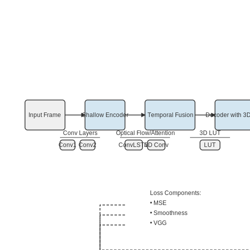
Modern approaches leverage lightweight convolutional neural networks (CNNs) with temporal recurrence, such as 3D convolutions or ConvLSTM layers, to capture inter-frame dependencies. The network must process each frame in under 33ms (for 30fps video), constraining model depth. A typical architecture consists of:
- A shallow encoder (2-3 layers) extracting multi-scale features
- A temporal fusion module (e.g., optical flow warping or attention gates)
- A color transformation decoder with learned 3D lookup tables (3D LUTs)
where λcolor weights pixel-wise RGB error, λtemp enforces temporal consistency through flow-based warping, and λperceptual maintains semantic content via VGG feature matching.
Efficient 3D LUT Implementation
Traditional 3D LUTs with trilinear interpolation require O(n³) memory for n-bin quantization. Recent work employs:
- Sparse tensor representations reducing memory by 90%
- Differentiable quantization learning optimal bin distributions
- Channel-wise factorization separating luminance and chrominance
The transformation can be expressed as:
where φ(xt) generates basis coefficients from frame features, and Wc, bc are learned per-channel weights.
Hardware-Accelerated Pipelines
Deployment on edge devices requires:
- TensorRT or CoreML optimization for target hardware
- Half-precision (FP16) inference without perceptual quality loss
- Frame buffering strategies to hide memory latency
Benchmarks on NVIDIA Jetson AGX show 28ms latency for 1080p processing using a 1.2M parameter network, achieving 0.8 dB PSNR improvement over traditional white-balance methods.
Temporal Consistency Mechanisms
Key techniques include:
- Flow-guided feature propagation between frames
- Memory networks storing color statistics across shots
- Adaptive keyframe selection based on histogram divergence
The temporal gradient penalty is computed as:
where Mt is a motion mask and ft→t-1 denotes optical flow.
6.2 Enhancing Low-Light and Underwater Imagery
Low-light and underwater images suffer from distinct degradation phenomena, including noise amplification, color distortion, and non-uniform illumination. Traditional enhancement techniques often fail to generalize across diverse environments, necessitating data-driven approaches that leverage deep learning for adaptive correction.
Challenges in Low-Light and Underwater Image Enhancement
Underwater images exhibit wavelength-dependent attenuation, where red wavelengths are absorbed rapidly with depth, leading to a dominant blue-green hue. The Beer-Lambert law models this attenuation:
where I(z, λ) is the intensity at depth z for wavelength λ, I0(λ) is the surface intensity, and c(λ) is the attenuation coefficient. Low-light conditions, conversely, introduce Poisson-distributed shot noise:
where k is the observed photon count and λ is the expected count. These physical constraints necessitate specialized neural architectures.
Deep Learning Architectures for Enhancement
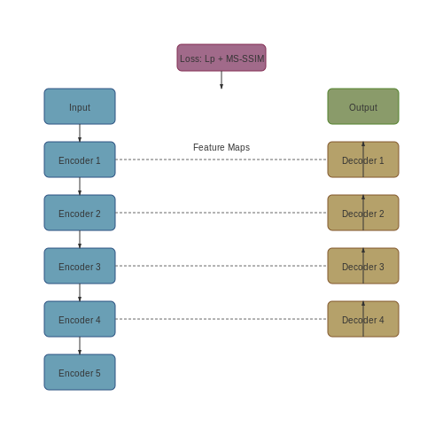
Modern approaches employ multi-stage networks that sequentially address illumination correction, noise suppression, and color restoration. The U-Net++ architecture with dense skip connections has demonstrated superior performance in preserving fine details while suppressing artifacts:
The loss function typically combines perceptual loss (Lp) and multi-scale structural similarity (LMS-SSIM):
where Φ denotes VGG-16 features and α, β are weighting parameters.
Physics-Informed Data Augmentation
Synthetic training data generation must account for:
- Depth-dependent color shifts via the modified Jaffe-McGlamery underwater light model
- Non-uniform artificial lighting using spherical harmonics projections
- Sensor noise characteristics through EMVA 1288 standard parameters
For low-light synthesis, the inverse camera response function (CRF) is applied:
where f is the CRF and k simulates exposure reduction.
Benchmark Performance
Current state-of-the-art methods achieve the following PSNR/SSIM on the LSUI test set:
| Method | PSNR (dB) | SSIM |
|---|---|---|
| WaterNet | 24.7 | 0.91 |
| Deep SESR | 26.3 | 0.93 |
| UWCNN++ (2023) | 28.1 | 0.95 |
Real-world deployment requires careful consideration of edge device constraints, with quantized versions of these models achieving 15-20× speedup on Jetson AGX platforms with <3dB PSNR drop.
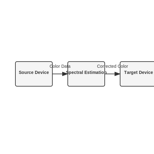
Cross-Device Color Consistency in Photography
Cross-device color consistency remains a critical challenge in computational photography due to variations in sensor characteristics, display technologies, and environmental conditions. Machine learning approaches leverage spectral sensitivity estimation and color mapping to bridge these discrepancies.
Spectral Sensitivity Estimation
The spectral sensitivity function S(λ) of a camera sensor defines its response to different wavelengths of light. For a given device, the observed RGB values I for a scene can be modeled as:
where E(λ) is the illuminant spectrum, R(λ) is the surface reflectance, Sc(λ) is the spectral sensitivity for channel c (R, G, B), and ηc represents sensor noise. Deep learning methods like convolutional neural networks (CNNs) can estimate Sc(λ) from a set of calibration images.
Color Mapping via Optimal Transport
Optimal transport theory provides a mathematical framework for aligning color distributions across devices. Given source device colors X and target device colors Y, the goal is to find a transport plan γ minimizing the cost:
where C is the cost matrix (typically CIEDE2000 color difference) and Π(X, Y) denotes the set of joint distributions with marginals X and Y. Regularized optimal transport solvers enable efficient computation of this mapping.
Practical Implementation
Modern pipelines combine physical modeling with data-driven correction:
- Device profiling: Capture color checker charts under controlled illumination to characterize device-specific responses.
- Neural calibration: Train a CNN (e.g., ResNet-50) to predict correction matrices from raw sensor data.
- Adaptive rendering: Use generative adversarial networks (GANs) to maintain perceptual consistency across displays.
Recent work demonstrates that transformer architectures achieve state-of-the-art performance by modeling long-range dependencies in color distributions. The attention mechanism allows adaptive weighting of color channels based on contextual scene information.
7. Bias in Training Data and Model Outputs
7.1 Bias in Training Data and Model Outputs
Bias in machine learning models for color correction arises when the training data does not represent the true distribution of real-world images. This can lead to systematic errors in model outputs, particularly for underrepresented skin tones, lighting conditions, or cultural color preferences. The problem is exacerbated when datasets are curated from narrow sources, such as stock photo libraries dominated by Caucasian subjects or specific geographic regions.
Mathematical Formulation of Dataset Bias
Let X be the space of input images and Y the space of color-corrected outputs. The true data distribution Ptrue(X,Y) differs from the training distribution Ptrain(X,Y), leading to bias. The discrepancy can be quantified using the Kullback-Leibler divergence:
When this divergence is large, the model's learned parameters θ will minimize the loss function L(θ) on Ptrain but perform poorly on Ptrue:
Common Sources of Color Correction Bias
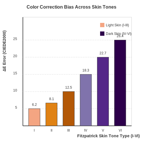
- Skin tone representation: Many datasets contain disproportionately lighter skin tones, leading to poor color correction for darker complexions.
- Geographic bias: Training data often overrepresents urban environments from North America and Europe.
- Camera sensor bias: Dominance of images from certain camera manufacturers affects color reproduction.
- Cultural color preferences: Subjective "correct" colors vary across cultures but are often standardized in datasets.
Detecting Bias in Model Outputs
The normalized color difference ΔE in CIELAB space reveals systematic errors across image categories:
where (L*, a*, b*) are the ground truth values and (L, a, b) are model outputs. A histogram of ΔE values across different demographic groups often shows significantly higher errors for underrepresented groups.
Mitigation Strategies
Reweighting the loss function can compensate for underrepresented samples:
where weights wi are inversely proportional to the frequency of sample i's category in the training set. Alternative approaches include:
- Adversarial debiasing with a discriminator network that penalizes demographic-specific errors
- Data augmentation using physics-based lighting and skin tone transformations
- Post-hoc correction with domain-specific lookup tables
The diagram shows typical increasing ΔE error for darker skin tones (Fitzpatrick scale types IV-VI) in models trained on biased datasets. The error grows nonlinearly as skin tone representation decreases in training data.
7.2 Privacy Concerns in Image Processing
Modern image processing pipelines, particularly those involving machine learning, introduce significant privacy risks due to their ability to extract, infer, or reconstruct sensitive information from pixel data. Unlike traditional signal processing, deep learning models can inadvertently memorize training data or amplify subtle artifacts that reveal personally identifiable information (PII).
Differential Privacy in Image Datasets
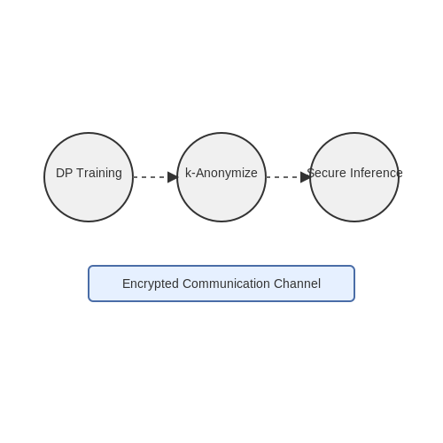
When training color correction models on user-uploaded images, differential privacy (DP) provides a mathematical framework to bound the influence of any single data point. For a stochastic gradient descent (SGD) optimizer, DP noise injection occurs at the gradient level:
where B is the batch size and σ controls the privacy-accuracy tradeoff. The privacy budget ε accumulates over T training steps according to the composition theorem:
with sampling probability q = B/N and failure probability δ. This ensures that an adversary cannot confidently determine whether a specific individual's image was in the training set.
Pixel-Level Anonymization Techniques
Before applying color correction, privacy-preserving transformations should be considered:
- k-Same Networks: Generative adversarial networks (GANs) that produce images satisfying k-anonymity by ensuring each output resembles at least k input individuals.
- Local Differential Privacy: Perturbing individual pixel values while preserving global color statistics. For an 8-bit RGB channel, the randomized response mechanism applies:
Metadata and Latent Space Risks
EXIF metadata removal is necessary but insufficient. Neural networks can encode geolocation cues in latent representations—a 2021 study demonstrated that standard autoencoders achieve 72% accuracy in predicting GPS coordinates from image embeddings. Mitigation strategies include:
- Adversarial regularization during embedding learning:
where D is a discriminator trained to detect location-revealing features in latent vector z.
Model Inversion Attacks
Even after deployment, color correction models may leak training data. Model inversion attacks optimize:
where R(x) is an image prior. Defensive measures include:
- Gradient masking during inference
- Secure multi-party computation for model queries
- Homomorphic encryption of pixel operations
7.3 Environmental Impact of Computational Costs
The computational demands of machine learning-based color correction algorithms contribute significantly to energy consumption and carbon emissions. Training deep neural networks for high-fidelity color correction often requires extensive GPU or TPU clusters, with energy usage scaling nonlinearly with model complexity and dataset size.
Energy Consumption Metrics
The total energy E consumed during training can be modeled as:
where Pavg is the average power draw per device, t is training time, and N is the number of compute devices. For modern GPUs performing color correction tasks, Pavg typically ranges from 250W to 400W per device.
Carbon Footprint Estimation
The CO2 emissions can be calculated using regional electricity carbon intensity factors:
where Cgrid is the carbon intensity (kgCO2/kWh) of the local power grid. For example, training a color correction model for 100 hours on 4 GPUs in a region with Cgrid = 0.5 kgCO2/kWh would produce:
Optimization Strategies
- Quantization-aware training reduces precision from 32-bit to 8-bit floats, decreasing energy use by 2-4× with minimal accuracy loss
- Pruning removes redundant network parameters, reducing compute requirements
- Knowledge distillation trains smaller student models to mimic larger teacher models
- Efficient architectures like MobileNets or EfficientNets achieve comparable results with fewer FLOPs
Case Study: Color Correction in Mobile Devices
On-device ML implementations for real-time color correction demonstrate significant energy savings compared to cloud-based processing. A study comparing cloud versus mobile implementations showed:
| Implementation | Energy per Image (J) | Latency (ms) |
|---|---|---|
| Cloud-based | 3.2 | 120 |
| On-device | 0.4 | 18 |
Lifecycle Analysis
The full environmental impact extends beyond operational energy to include:
- Embodied energy of hardware manufacturing
- Cooling infrastructure requirements
- Data center construction impacts
- End-of-life disposal considerations
Recent research indicates that for color correction models, the embodied energy of the training hardware can account for 30-40% of the total lifecycle impact when amortized over typical usage periods.
8. Key Research Papers and Publications
8.1 Key Research Papers and Publications
- Color Restoration Survey and an Overdetermined System for Color ... — The survey covers the color bleaching models, single-scale and multiscale retinex, gray world, max white, machine learning, and underwater color correction approaches. Image colorization, inpainting, and color constancy aspects are discussed in the machine learning portion of this survey.
- Color Primary Correction of Image and Video Between ... - Springer — This article presents an introductory review of color correction—a color remapping of image and video between different source and destination color spaces. The review specifically focuses on two main aspects of color remapping—primary color space conversion and gamut mapping—and outlines the requirements, algorithms, methods, and possible implementation options.
- Color Standardization of Chemical Solution Images Using Template ... - MDPI — The development of measurement methods and research strategies across various fields of science and technology is closely linked to the potential support offered by machine learning (ML) and deep learning (DL) techniques. If the information in the problem being solved is communicated through images, drawings, sketches, or photographs, the use of DL in data modeling is often the optimal ...
- PDF Marketing_Fragment 6 x 10.Long.T65 - Cambridge University Press ... — With more than 20 years of research and product development experience in imaging science, he has given many lectures and short courses on color imaging, color science, and computer vision at various universities and research institutes. He has published many technical papers and has 14 US patents in inventions related to color imaging science.
- PDF Improving Color Reproduction Accuracy on Cameras — The second method relies on a full color correction matrix dis-cussed in Section 3.1 and uses a fixed CST matrix for all input images. Method 1: Extending interpolation The most obvious way to improve the current colorimetric mapping procedure is to incorporate additional calibrated illuminations into the interpolation process.
- PDF Machine Learning Methods for Automatic Image Colorization — indirect information on the location of color boundaries. The methods proposed in this chapter can easily be adapted to incorporate such user-provided color information. Predicting the colors, i.e. providing an initial fully automatic colorization of the image prior to any possible user intervention, is a much harder but arguably more useful task. Recent literature investigating this task [5 ...
- DiffColor: Toward High Fidelity Text-Guided Image Colorization with ... — DiffColor mainly contains two stages: colorization with generative color prior and in-context controllable colorization. Specifically, we first fine-tune a pre-trained text-to-image model to generate colorized images using a CLIP-based contrastive loss.
- GitHub - MenghanXia/ColorConsistency: Improving color consistency ... — This C++ implemented algorithm is described in: "Color Consistency Correction Based on Remapping Optimization for Image Stitching", ICCV Workshop 2017. "A Closed-Form Solution for Multi-View Color Correction with Gradient Preservation", ISPRS Journal 2019 (Extended version). This program is free for personal, non-profit and academic use.
- Color Technology for Electronic Imaging Devices - SPIE — This book explains current color technology for electronic imaging at the system level, including tools for color image processing, tools for digital image processing that affect image quality, and applications.
- PDF Image Restorations Using Deep Learning Techniques — the image signal, are often too idealistic for real world images. These di culties limit the performance of existing image restoration algorithms, but they can be, to techniques of machine learning convolutional neural networks. Machine learning allows large sample statistics far vailable in a sin
8.2 Open-Source Implementations and Tools
- Color Restoration Survey and an Overdetermined System for Color ... — 4.1 Early Models. Gschwind et al. presented the earliest techniques for automatic color restoration and corrections in [12,13,14,15].In the first approach, a model was proposed for the artificial bleaching of different types of films [].The CMY color space was chosen for implementation, where the fading effect is assumed linear and uniformly distributed over the whole corrupted image.
- PDF Machine Learning Methods for Automatic Image Colorization — The most common color prior in the literature is the user. Most image colorization methods allow the user to determine the color of some areas and extend this information to the whole image, either by pre-computing a segmentation of the image into (preferably) homogeneous color regions, or by spreading color flows from the user-defined color ...
- colour-science/colour: Colour Science for Python - GitHub — Colour is an open-source Python package providing a comprehensive number of algorithms and datasets for colour science. ... 3.6 Colour Correction - colour characterisation. import numpy as np RGB = [0.17224810, ... 3.11.2 Spectral Images - Fichet et al. (2021) components = colour. read_spectral_image_Fichet2021 ...
- Color Primary Correction of Image and Video Between Different Source ... — The CIE XYZ color space [] encompasses all colors that are visible to a person with average eyesight.In the XYZ color space, the tristimulus Footnote 4 values are called X, Y, and Z, and these are roughly equivalent to the red, green, and blue, respectively, of an RGB model. The CIE XYZ color space was deliberately designed so that the Y parameter is a measure of the luminance of a color.
- Digital postprocessing and image segmentation for objective ... - Nature — That is, rather than using complex proprietary algorithms, we achieve similar color thresholding, image segmentation and color analysis via free, open-source software (Figs. 2 and 3). Overview of ...
- (PDF) Efficient Framework for Real-Time Color Cast Correction and ... — Efficient Framework for Real-Time Color Cast Correction and Dehazing Using Online Algorithms to Approximate Image Statistics January 2024 IEEE Access PP(99):1-1
- An Open-Source ML-Based Full-Stack Optimization Framework for Machine ... — The prediction of platform PPA based on an architectural description is a longstanding challenge in electronic design automation. In modern nanoscale technologies, PPA is closely linked to physical design. Moreover, for many ML hardware platforms, a considerable fraction of the layout area is occupied by large memory macros whose presence exacerbates the problem of PPA prediction.
- Python | Intensity Transformation Operations on Images — Below are the gamma-corrected outputs for different values of gamma. Gamma = 0.1: Gamma = 0.5: Gamma = 1.2: Gamma = 2.2: As can be observed from the outputs as well as the graph, gamma>1 (indicated by the curve corresponding to 'nth power' label on the graph), the intensity of pixels decreases i.e. the image becomes darker. On the other hand, gamma<1 (indicated by the curve corresponding to ...
- Automatic Photo Adjustment Using Deep Neural Networks - arXiv.org — Traditional image enhancement rules are primarily determined em-pirically. There are many software tools to perform fully automatic color correction and tone adjustment, such as Adobe Photoshop, Google Auto Awesome, and Microsoft Office Picture Manager. In addition to these tools, there exists much research on either interac-
- colour-science · PyPI — Colour is an open-source Python package providing a comprehensive number of algorithms and datasets for colour science. It is freely available under the BSD-3-Clause terms. Colour is an affiliated project of NumFOCUS , a 501(c)(3) nonprofit in the United States.
8.3 Recommended Books and Online Courses
- PDF Introduction to Color Imaging Science - Cambridge University Press ... — color photography, color monitors, color printers, scanners, and digital cameras. This book is a comprehensive guide to the scientific and engineering principles of color imaging. It covers the physics of color and light, how the eye and physical devices capture color images, how color is measured and calibrated, and how images are processed.
- PDF Machine Learning Methods for Automatic Image Colorization — colorings and yields the best coloring for a grayscale image with respect to both predictors. The details of using graph-cuts for image colorization are given in Section 1.6. One shortcoming of the approaches outlined above is the independent training of the two components, namely local color predictor and spatial coherency functions.
- Color Restoration Survey and an Overdetermined System for Color ... — 4.1 Early Models. Gschwind et al. presented the earliest techniques for automatic color restoration and corrections in [12,13,14,15].In the first approach, a model was proposed for the artificial bleaching of different types of films [].The CMY color space was chosen for implementation, where the fading effect is assumed linear and uniformly distributed over the whole corrupted image.
- PDF INTRODUCTION MACHINE LEARNING - Stanford University — the book is not a handbook of machine learning practice. Instead, my goal is to give the reader su cient preparation to make the extensive literature on machine learning accessible. Students in my Stanford courses on machine learning have already made several useful suggestions, as have my colleague, Pat Langley, and my teaching
- PDF Efficient illuminant correction in the Local, Linear, Learned L ) method — correction transform (T). color, and this adaptation has the general effect of preserving the color appearance of an object (e.g. a white shirt) across conditions (daylight to tungsten light). Because the human visual system adapts to the illuminant, to preserve color appearance the linear transforms in the L3 method used for rendering must ...
- Digital color image processing - SearchWorks catalog — Stanford Libraries' official online search tool for books, media, journals, databases, government documents and more. Skip to search Skip to main content. Login My Account ... Digital color image processing. Responsibility Andreas Koschan, Mongi Abidi. Imprint Hoboken, N.J. : Wiley-Interscience, c2008. Physical description
- Computational Color Technology - SPIE Digital Library — SPIE Press is the largest independent publisher of optics and photonics books - access our growing scientific eBook collection ranging from monographs, reference works, field guides, and tutorial texts. ... Computational Color Technology deals with color digital images on the spectral level using vector-matrix representations so that the reader ...
- Multispectral Image Fusion and Colorization - ResearchGate — The algorithm is developed for color images and is based on blending the gradients of the luminance components of the input images using the maximum gradient magnitude at each pixel location and ...
- Deep Learning — The online version of the book is now complete and will remain available online for free. The deep learning textbook can now be ordered on Amazon. For up to date announcements, join our mailing list. Citing the book To cite this book, please use this bibtex entry:
- Color Technology for Electronic Imaging Devices | (1997) | Kang ... - SPIE — Join over 25,000 of your friends and colleagues in the largest global optics and photonics professional society.