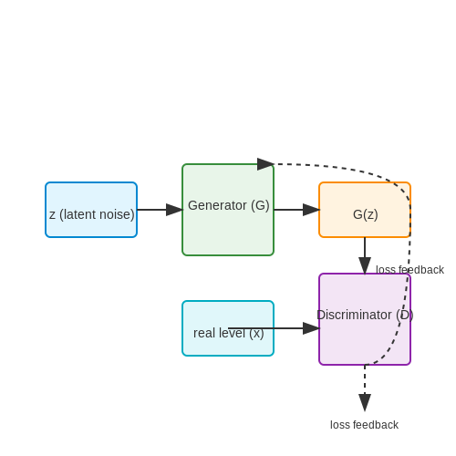
Conditional GANs (cGANs) Explained
1. Core Concept: Conditional Generation in GANs
1.1 Core Concept: Conditional Generation in GANs
Conditional Generative Adversarial Networks (cGANs) extend the standard GAN framework by introducing auxiliary information y to condition both the generator G and discriminator D. This conditioning enables controlled generation of samples that adhere to specified attributes, such as class labels, text descriptions, or structured data. The key innovation lies in modifying the original GAN objective function to incorporate this conditional information:
Here, y represents the conditioning variable, which is concatenated with the noise vector z in the generator and with the input data in the discriminator. This architectural modification forces the generator to learn a mapping from (z, y) to x that is coherent with the specified conditions, while the discriminator must evaluate both the authenticity of samples and their consistency with y.
Architectural Implementation
The conditioning is typically implemented through:
- Concatenation: Directly appending y to the input noise vector z in the generator and to the input data in the discriminator.
- Embedding layers: For discrete labels, an embedding layer projects y into a continuous space before concatenation.
- Attention mechanisms: In more advanced architectures, attention can be used to dynamically weight the influence of different parts of y.
Mathematical Derivation of the cGAN Objective
The cGAN objective can be derived by considering the conditional distributions. Let pdata(x|y) be the true conditional data distribution and pG(x|y) the generator's learned distribution. The discriminator aims to distinguish between samples from these distributions:
Substituting this optimal discriminator back into the value function yields:
where DJS is the Jensen-Shannon divergence. This shows that the generator is trained to minimize the JS divergence between the conditional distributions.
Practical Applications
cGANs have demonstrated remarkable success in several domains:
- Image-to-image translation: Pix2Pix uses paired data to learn mappings between image domains conditioned on input images.
- Text-to-image synthesis: StackGAN generates photorealistic images from text descriptions by conditioning on embedded text features.
- Medical imaging: cGANs can generate specific anatomical structures conditioned on segmentation masks.
Challenges and Limitations
While powerful, cGANs present several challenges:
- Mode collapse: The generator may ignore the conditioning information and produce limited varieties of outputs.
- Training instability: The adversarial training process remains delicate, requiring careful tuning of hyperparameters.
- Conditional information leakage: Poorly designed architectures may allow the generator to ignore the conditioning input.
Recent advances like projection discriminators and auxiliary classifier GANs (AC-GANs) have addressed some of these limitations by more effectively incorporating conditional information throughout the network architecture.

Architecture Overview: Generator and Discriminator with Conditions
Conditional GANs (cGANs) extend the standard GAN framework by incorporating auxiliary information y—such as class labels, text embeddings, or structured data—into both the generator G and discriminator D. This conditioning enables targeted generation and adversarial evaluation, transforming the unsupervised GAN into a supervised or semi-supervised model.
Conditional Generator Architecture
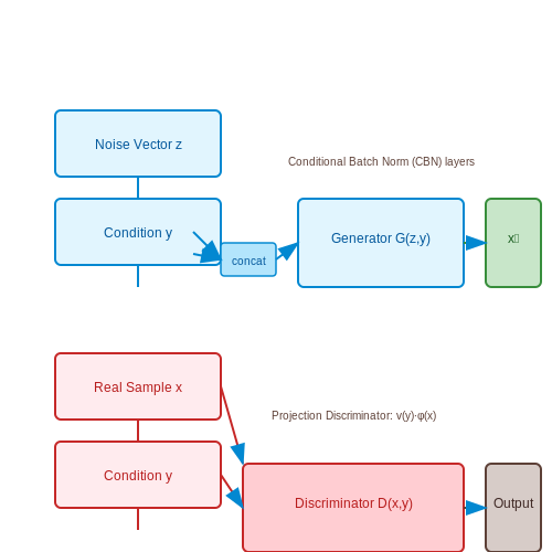
The generator G(z, y) maps a noise vector z and condition y to a synthetic sample x̃. The condition y is typically concatenated with z at the input layer, though advanced variants use projection or attention mechanisms. For a generator with L layers, the forward pass becomes:
In practice, conditions are often embedded into intermediate layers via conditional batch normalization (CBN), where the normalization parameters γ and β are dynamically generated from y:
Conditional Discriminator Architecture
The discriminator D(x, y) evaluates whether x is real or synthetic while enforcing consistency with y. Common implementations use:
- Concatenation-based discriminators: y is concatenated with x or intermediate feature maps.
- Projection discriminators: Inner products between embedded conditions and feature vectors are added to the final logits.
- Auxiliary classifiers: A separate branch predicts y to enforce semantic alignment.
The projection discriminator’s objective formalizes this as:
where v(y) is a condition embedding, φ(x) denotes deep features, and ψ is a scalar function.
Training Dynamics
The minimax objective incorporates conditions via:
Gradient penalties or spectral normalization are often applied to stabilize training. The discriminator’s ability to reject samples with mismatched conditions (e.g., generating a "cat" when y requests a "dog") is critical for mode disentanglement.
Architectural Variants
Conditional GANs exhibit design flexibility across domains:
- Image synthesis: Stacked generators progressively refine resolution (e.g., 64×64 → 256×256) with spatially-adaptive normalization.
- Text-to-image: Attention mechanisms align textual y with image regions.
- Medical imaging: Anatomical constraints are encoded via segmentation masks in y.
1.3 Key Differences Between cGANs and Standard GANs
Conditional Input Integration
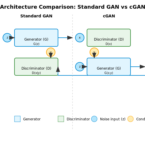
Standard GANs generate samples from random noise z sampled from a prior distribution, typically Gaussian or uniform. The generator G learns a mapping G: z → x, where x is the generated sample. In contrast, conditional GANs (cGANs) incorporate auxiliary information y (e.g., class labels, text embeddings, or structured data) as an additional input to both the generator and discriminator. The mapping becomes G: (z, y) → x, enabling controlled generation.
Discriminator Conditioning
The discriminator D in a standard GAN evaluates the authenticity of a sample x alone, whereas in cGANs, it assesses the joint probability of the sample x and the condition y. The discriminator's objective shifts from D(x) to D(x|y), enforcing alignment between generated samples and their conditions.
Loss Function Formulation
The adversarial loss in standard GANs is:
For cGANs, the loss incorporates the conditional variable y:
Mode Collapse Mitigation
Standard GANs are prone to mode collapse, where the generator produces limited varieties of samples. cGANs mitigate this by leveraging the conditional input y to explicitly diversify outputs. For instance, in image generation, conditioning on class labels ensures coverage across all specified categories.
Applications and Flexibility
While standard GANs excel in unsupervised tasks like image synthesis, cGANs enable task-specific generation, such as:
- Text-to-image synthesis (e.g., generating images from captions)
- Image-to-image translation (e.g., converting sketches to photos)
- Class-conditional generation (e.g., creating MNIST digits of a specified class)
Training Dynamics
cGANs often require more careful balancing between the generator and discriminator due to the added complexity of conditioning. The discriminator must learn to reject samples that are realistic but misaligned with the condition y, which can slow convergence compared to standard GANs.
Architectural Variations
Conditional information y can be integrated into the network in multiple ways:
- Concatenation: y is concatenated with the noise vector z at the generator's input and with the sample x at the discriminator's input.
- Embedding Layers: y is projected into a learned embedding space before integration.
- Attention Mechanisms: In advanced architectures like AttnGAN, conditions modulate feature maps via attention.
2. Objective Function and Conditional Loss
Objective Function and Conditional Loss
The objective function of a conditional Generative Adversarial Network (cGAN) extends the standard GAN framework by incorporating auxiliary information, typically in the form of class labels or structured data, to guide the generation process. The key distinction lies in the conditioning of both the generator G and the discriminator D on this additional information y.
Conditional Adversarial Loss
The adversarial loss for cGANs modifies the original GAN objective by introducing the conditional variable y. The minimax game between G and D is formulated as:
Here, x represents real data samples, z is the noise vector, and y is the conditioning variable. The generator G learns to produce samples that are not only realistic but also consistent with the given condition y, while the discriminator D evaluates whether the sample is both real and matches the condition.
Derivation of the Conditional Objective
The conditional loss can be derived by examining the optimal discriminator for a fixed generator. For a given G, the discriminator D aims to maximize:
By taking the functional derivative with respect to D and setting it to zero, the optimal discriminator D* is obtained as:
where pg(x|y) is the generator's distribution conditioned on y. Substituting D* back into the objective yields the conditional version of the Jensen-Shannon divergence:
Practical Implementation Considerations
In practice, the conditional information y is often concatenated with the input noise vector z for the generator and with the input data for the discriminator. For high-dimensional conditions (e.g., text or images), y is typically embedded into a lower-dimensional space before concatenation.
The gradient updates for G and D must account for the conditioning, which can be implemented efficiently using modern deep learning frameworks. The discriminator's loss function becomes:
while the generator's loss is:
Extensions and Variants
Several variants of the conditional loss have been proposed to improve training stability and sample quality. The projection discriminator introduces an inner product between the embedded condition and intermediate features, while auxiliary classifier GANs (AC-GANs) add a classification loss to ensure condition consistency.
2.2 Training Dynamics and Convergence
Objective Function and Nash Equilibrium
The training dynamics of cGANs are governed by a minimax game between the generator G and discriminator D, conditioned on auxiliary information y. The objective function extends the standard GAN formulation:
Convergence occurs when the generator’s distribution pg matches the data distribution pdata, achieving a Nash equilibrium. However, in practice, this equilibrium is rarely stable due to the non-convex nature of the optimization landscape.
Mode Collapse and Gradient Issues
Two critical challenges in cGAN training are:
- Mode Collapse: The generator produces limited varieties of samples, ignoring other modes of the data distribution.
- Vanishing Gradients: When the discriminator becomes too strong, gradients for the generator diminish, halting learning.
These issues are exacerbated in cGANs due to the additional conditioning constraints. Techniques like feature matching and minibatch discrimination help mitigate them.
Conditional Training Stability
The discriminator in cGANs must learn to evaluate both the realism of samples and their alignment with the condition y. This dual objective introduces additional training instability. A common solution is to use:
where the discriminator is trained to distinguish real pairs (x, y) from fake pairs (G(z|y), y).
Empirical Convergence Strategies
Several empirically validated strategies improve cGAN convergence:
- Label Smoothing: Replace hard labels (0/1) with smoothed values (e.g., 0.1/0.9) to prevent discriminator overconfidence.
- Two-Timescale Update Rule (TTUR): Use different learning rates for G and D to balance their training.
- Spectral Normalization: Constrain the Lipschitz constant of the discriminator to stabilize training.
Monitoring Convergence
Unlike traditional GANs, cGANs require monitoring both sample quality and condition adherence. Common metrics include:
- Inception Score (IS): Measures diversity and quality of generated samples.
- Frechet Inception Distance (FID): Compares statistics of real and generated samples.
- Conditional Consistency: Ensures generated samples align with the given condition y.
These metrics, combined with qualitative inspection, provide a robust assessment of convergence.
Mode Collapse and Conditioning
Mode collapse occurs when a GAN's generator produces a limited subset of possible outputs, ignoring the full diversity of the training data distribution. In standard GANs, this manifests as the generator converging to a few modes (e.g., generating nearly identical samples), failing to capture the true data manifold. Conditional GANs (cGANs) mitigate this issue by leveraging auxiliary information (e.g., class labels or attributes) to guide the generation process, enforcing structured diversity.
Mechanisms of Mode Collapse
The root cause lies in the adversarial training dynamics: if the discriminator fails to penalize the generator for producing limited variations, the generator exploits this weakness by collapsing to high-confidence outputs. Mathematically, this can be analyzed through the generator's objective:
When mode collapse occurs, the generator optimizes for a subset of inputs z that reliably fool the discriminator, neglecting other regions of the latent space. The discriminator, in turn, becomes overspecialized to detect only the collapsed modes, creating a feedback loop.
Conditioning as a Stabilizing Factor
cGANs introduce conditional variables y (e.g., class labels) to both generator and discriminator, modifying the objective:
By conditioning on y, the generator must produce outputs that align with specific constraints, preventing trivial solutions. For example, in a cGAN trained on MNIST, the label y forces the generator to produce distinct digits rather than collapsing to a single digit. The discriminator’s conditional feedback ensures that samples are both realistic and consistent with y.
Empirical Observations
- Label Smoothing: Replacing hard labels (0/1) with soft targets (e.g., 0.1/0.9) reduces discriminator overconfidence, discouraging mode collapse.
- Mini-batch Discrimination: Comparing samples within a batch helps the discriminator detect redundancy, penalizing generators that produce similar outputs.
- Architectural Constraints: Techniques like spectral normalization or gradient penalty (e.g., Wasserstein GAN) stabilize training by limiting discriminator capacity.
Practical Implications
In applications like medical imaging or text-to-image synthesis, mode collapse can lead to catastrophic failures (e.g., generating only one type of tumor morphology or a single image variation). cGANs address this by tying generated samples to explicit conditions, ensuring coverage of the target distribution. For instance, in the Pix2Pix framework, the input sketch conditions the output image, preventing degenerate solutions.
Here, the generator G must not only fool the discriminator but also adhere to the paired input-output relationship enforced by x (e.g., edges→photos). This dual requirement inherently diversifies outputs.
3. Data Preparation and Conditioning Strategies
Data Preparation and Conditioning Strategies
Conditional GANs (cGANs) require careful data preparation and conditioning to ensure the generator learns meaningful mappings between input conditions and output distributions. Unlike standard GANs, cGANs incorporate auxiliary information y (e.g., class labels, text embeddings, or structured metadata) to guide the generation process. The conditioning strategy must preserve the relationship between y and the data distribution p(x|y) while avoiding mode collapse or overfitting.
Conditional Data Pairing
The core challenge lies in constructing paired samples (x, y) where x is the data instance and y is its corresponding condition. For discrete labels (e.g., MNIST digits), this is straightforward:
For continuous conditions (e.g., regression targets or time-series embeddings), normalization is critical to stabilize training:
Embedding Strategies
High-dimensional conditions (e.g., text or graphs) require embedding layers to project y into a latent space compatible with the generator G and discriminator D. Common approaches include:
- Learnable embeddings: A trainable lookup table for discrete labels, optimized end-to-end with the GAN loss.
- Pretrained encoders: Fixed embeddings from models like BERT (text) or ResNet (images), reducing dimensionality while preserving semantics.
- Attention-based conditioning: Cross-attention layers in G to dynamically weight condition features.
Architectural Conditioning Methods
The method of injecting y into G and D significantly impacts performance. Three dominant strategies exist:
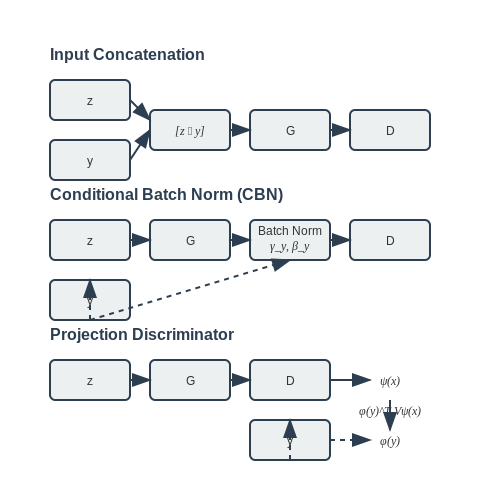
1. Input Concatenation
Append y to the generator’s noise vector z and the discriminator’s input x:
This requires matching dimensions via padding or projection but can lead to weak condition adherence if y is overshadowed by other inputs.
2. Conditional Batch Normalization (CBN)
Modify batch normalization layers in G to use condition-dependent scaling parameters:
where γy, βy are learned affine transformations conditioned on y. This is particularly effective for style transfer tasks.
3. Projection Discriminator
Introduced by Miyato & Koyama (2018), this method computes the inner product between embedded conditions and data features:
where ψ and ϕ are embedding networks, and V is a learnable matrix. This enforces tighter condition-data coupling.
Data Augmentation for cGANs
Conditional data augmentation prevents overfitting when training data is limited. Techniques include:
- Condition-preserving transforms: Rotations/flips for images where y is invariant to the transformation.
- Mixup conditioning: Linear interpolation of conditions and data pairs (x_i, y_i) and (x_j, y_j).
- Adversarial augmentation: Using a small GAN to generate synthetic (x, y) pairs that fool D.
In medical imaging cGANs, for instance, synthetic tumor masks (y) paired with MRI scans (x) are augmented via elastic deformations that preserve anatomical constraints.
3.2 Building a cGAN with TensorFlow/PyTorch
Architecture Overview
The conditional GAN extends the standard GAN framework by incorporating auxiliary information y as input to both generator G and discriminator D. The objective function becomes:
Where y represents the conditional information (e.g., class labels) concatenated with either the noise vector z (for G) or the real/fake samples (for D).
TensorFlow Implementation
The generator network typically uses transposed convolutions for upsampling:
def build_generator(latent_dim, num_classes):
    noise = Input(shape=(latent_dim,))
    label = Input(shape=(1,), dtype='int32')

    # Embed labels and multiply with noise
    label_embedding = Flatten()(Embedding(num_classes, latent_dim)(label))
    model_input = multiply([noise, label_embedding])

    # Generator architecture
    x = Dense(128 * 7 * 7)(model_input)
    x = Reshape((7, 7, 128))(x)
    x = Conv2DTranspose(128, (4,4), strides=2, padding='same')(x)
    x = BatchNormalization()(x)
    x = LeakyReLU(alpha=0.2)(x)
    x = Conv2DTranspose(64, (4,4), strides=2, padding='same')(x)
    x = BatchNormalization()(x)
    x = LeakyReLU(alpha=0.2)(x)
    outputs = Conv2D(1, (7,7), activation='tanh', padding='same')(x)

    return Model([noise, label], outputs)
PyTorch Implementation
The discriminator uses conditional batch normalization and label information:
class Discriminator(nn.Module):
    def __init__(self, num_classes):
        super().__init__()
        self.label_embedding = nn.Embedding(num_classes, img_size * img_size)

        self.model = nn.Sequential(
            nn.Conv2d(2, 64, 4, 2, 1),
            nn.LeakyReLU(0.2, inplace=True),
            nn.Conv2d(64, 128, 4, 2, 1),
            nn.BatchNorm2d(128),
            nn.LeakyReLU(0.2, inplace=True),
            nn.Conv2d(128, 256, 4, 2, 1),
            nn.BatchNorm2d(256),
            nn.LeakyReLU(0.2, inplace=True),
            nn.Conv2d(256, 1, 4, 1, 0),
            nn.Sigmoid()
        )

    def forward(self, img, labels):
        label_embed = self.label_embedding(labels).view(labels.size(0), 1, img_size, img_size)
        concat_input = torch.cat((img, label_embed), dim=1)
        return self.model(concat_input)
Training Dynamics
The training loop implements the modified minimax game with conditional inputs:
Key implementation details:
- Label smoothing: Replace 1.0 with 0.9 for real samples to prevent overconfidence
- Noise injection: Add Gaussian noise to discriminator inputs for stability
- Feature matching: Use intermediate layer activations as additional loss terms
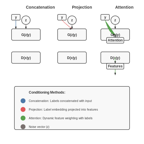
Conditioning Techniques
Three primary methods exist for incorporating conditional information:
- Concatenation: Directly append y to input vectors
- Projection: Use matrix multiplication to combine features (as in the TensorFlow example)
- Attention: Employ cross-attention mechanisms for dynamic feature weighting
Hyperparameter Optimization
Critical parameters for stable training:
| Parameter | Recommended Value | Effect |
|---|---|---|
| Learning Rate | 2e-4 (G), 5e-5 (D) | Controls update step size |
| Batch Size | 32-128 | Affects gradient variance |
| β1 (Adam) | 0.5 | Momentum term |
3.3 Hyperparameter Tuning and Optimization
Learning Rate and Optimizer Selection
The learning rate (η) is a critical hyperparameter in cGAN training, influencing both convergence speed and stability. A common starting point is η = 0.0002, as empirically validated in the original DCGAN paper. However, adaptive optimizers like Adam often outperform SGD due to their momentum-based updates. The Adam optimizer’s parameters (β₁, β₂) should be tuned carefully:
where θ represents the model parameters, m̂ₜ and v̂ₜ are bias-corrected first and second moment estimates, and ϵ is a small constant for numerical stability. Typical values are β₁ = 0.5, β₂ = 0.999, though recent work suggests β₁ = 0.0 can improve stability for GANs.
Batch Normalization and Layer-Specific Adjustments
Batch normalization (BN) is often used in cGANs to stabilize training, but its parameters require careful tuning. The momentum term in BN layers (default 0.9) controls the exponential moving average of batch statistics. For conditional generation tasks, instance normalization or spectral normalization may outperform BN by reducing mode collapse. Layer-specific learning rate multipliers can further refine training:
- Generator: Lower learning rates (e.g., 0.5× base rate) prevent overshooting.
- Discriminator: Higher rates (e.g., 2× base rate) maintain adversarial pressure.
Architecture-Specific Hyperparameters
The depth and width of cGAN architectures directly affect their capacity. For ResNet-based generators, the number of residual blocks (n_blocks) should scale with output resolution:
where h_out is the output height and h_latent is the latent space dimension. Channel multipliers in convolutional layers typically follow geometric progression (e.g., [64, 128, 256, 512]).
Loss Function Weighting
Conditional GANs often employ multi-term loss functions (e.g., adversarial loss + L1 reconstruction loss). The weighting factor λ balances these objectives:
Empirical studies show λ = 100 works well for image-to-image translation tasks. For Wasserstein GAN variants, the gradient penalty coefficient (λ_GP) is typically set to 10.
Training Dynamics Monitoring
Advanced monitoring techniques include:
- Gradient norms: Discriminator gradients should remain bounded (WGAN-GP recommends ‖∇D‖₂ ≈ 1).
- Inception Score (IS) or Fréchet Inception Distance (FID): Tracked every k iterations (e.g., k=1000).
- Conditional entropy: Measures how well the generator respects input conditions.
Early stopping criteria can be based on FID plateaus (e.g., no improvement for 20 epochs). Mixed-precision training (fp16) often accelerates convergence while maintaining stability.
4. Image-to-Image Translation (e.g., Pix2Pix)
Image-to-Image Translation (e.g., Pix2Pix)
Image-to-image translation with conditional GANs (cGANs) involves learning a mapping from an input image x to an output image y, conditioned on a structured input. The Pix2Pix framework, introduced by Isola et al. (2017), formalizes this as a supervised learning problem where paired training data (x, y) is available. The generator G learns to produce realistic outputs that match the target distribution, while the discriminator D distinguishes between real and generated pairs.
Objective Function
The Pix2Pix objective combines a conditional adversarial loss with an L1 reconstruction loss to enforce pixel-wise similarity:
The full objective is a weighted sum of these terms:
where λ controls the trade-off between adversarial training and reconstruction fidelity.
Architecture Details
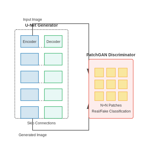
Pix2Pix employs a U-Net architecture for the generator, which preserves high-frequency details through skip connections between encoder and decoder layers. The discriminator uses a PatchGAN structure, classifying local image patches rather than the entire image, which improves training stability and output quality.
U-Net Generator
The U-Net consists of:
- An encoder with strided convolutions for downsampling.
- A decoder with transposed convolutions for upsampling.
- Skip connections that concatenate encoder feature maps to decoder layers.
PatchGAN Discriminator
The discriminator operates on N×N patches, where N is typically 70×70. This design:
- Reduces computational cost compared to full-image discriminators.
- Encourages high-frequency detail preservation.
- Produces sharper outputs by focusing on local texture realism.
Training Dynamics
Training proceeds in alternating steps:
- The discriminator D is updated to maximize its ability to distinguish real pairs (x, y) from fake pairs (x, G(x)).
- The generator G is updated to minimize the adversarial loss while also minimizing the L1 distance between G(x) and y.
Batch normalization and dropout are applied in both networks to stabilize training. The Adam optimizer with a learning rate of 0.0002 and momentum parameters β₁ = 0.5, β₂ = 0.999 is typically used.
Applications and Extensions
Pix2Pix has been successfully applied to:
- Semantic segmentation ↔ Photo synthesis (e.g., generating street views from labels).
- Sketch-to-image translation (e.g., converting architectural drawings to realistic renders).
- Medical imaging (e.g., generating CT scans from MRI data).
Extensions like CycleGAN relax the paired data requirement by introducing cycle-consistency losses, while newer approaches like SPADE (GauGAN) incorporate spatially-adaptive normalization for higher-quality synthesis.
Limitations
Key challenges include:
- Dependence on paired training data for optimal performance.
- Difficulty handling multi-modal outputs (a single input may correspond to multiple valid outputs).
- Sensitivity to hyperparameters, particularly the adversarial/L1 loss weighting factor λ.
Text-to-Image Synthesis
Text-to-image synthesis using conditional GANs (cGANs) involves generating photorealistic images from textual descriptions by conditioning the generator and discriminator on embedded text features. The core challenge lies in aligning high-dimensional visual outputs with semantically meaningful text embeddings while maintaining adversarial training stability.
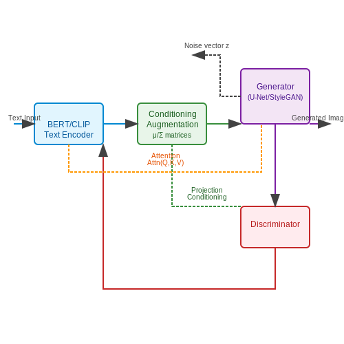
Architecture Overview
Modern text-to-image cGANs typically employ a hierarchical architecture:
- Text Encoder: A pre-trained language model (e.g., BERT, CLIP) projects input text into a latent embedding space.
- Conditioning Augmentation: Transforms text embeddings into stochastic conditioning vectors via:
where t is the text embedding, and μ, Σ are learned mean and covariance matrices.
- Generator: A U-Net or StyleGAN variant upsamples noise vectors conditioned on c through multiple resolution blocks.
- Discriminator: Jointly processes image patches and text embeddings via projection-based conditioning.
Adversarial Objective
The minimax game incorporates text-image matching through:
with z as noise vector and x as real images. State-of-the-art implementations like AttnGAN introduce attention mechanisms between text tokens and image regions:
Training Dynamics
Key stabilization techniques include:
- Multi-scale discriminators to capture global and local coherence
- Adaptive gradient penalty for Lipschitz continuity
- Pre-trained text encoders frozen during GAN training
Empirical studies show that KL divergence between conditional and marginal distributions should remain below 0.5 nats to prevent mode collapse. The Fréchet Inception Distance (FID) between generated and real image distributions typically serves as the primary metric:
Applications and Limitations
Current systems achieve photorealistic synthesis for constrained domains (e.g., birds, flowers) but struggle with:
- Compositional reasoning (e.g., "a red cube on a blue sphere")
- Physical plausibility in complex scenes
- Fine-grained attribute control
Recent breakthroughs like DALL-E 2 and Imagen demonstrate that scaling transformer-based text encoders alongside diffusion models can surpass traditional cGAN approaches in open-domain settings.
4.3 Medical Imaging and Other Domain-Specific Uses
Conditional GANs (cGANs) have demonstrated remarkable success in medical imaging, where precise and high-fidelity synthetic data generation is critical. Unlike traditional GANs, cGANs leverage auxiliary information—such as segmentation masks, class labels, or multi-modal inputs—to generate anatomically plausible images. This capability is particularly valuable in scenarios where labeled medical datasets are scarce or privacy concerns restrict data sharing.
Medical Image Synthesis
In medical imaging, cGANs are widely used for tasks such as:
- Data Augmentation: Generating synthetic MRI or CT scans conditioned on lesion masks to improve the robustness of diagnostic models.
- Cross-Modal Translation: Converting MRI to CT scans (or vice versa) by conditioning on paired or unpaired datasets, reducing the need for redundant imaging.
- Super-Resolution: Enhancing low-resolution ultrasound or X-ray images by conditioning on high-resolution reference patches.
The objective function for a cGAN in medical image synthesis extends the standard GAN loss with conditioning. The generator G and discriminator D optimize:
where y represents the conditioning variable (e.g., a segmentation mask or modality label).
Domain-Specific Challenges
Medical applications impose unique constraints on cGANs:
- Anatomical Consistency: Generated images must adhere to physiological plausibility. Techniques like gradient penalty or perceptual loss are often incorporated to enforce this.
- Small Dataset Adaptation: Transfer learning from natural images to medical domains is limited due to domain shift. Hybrid architectures, such as U-Net-based generators, are common.
- Multi-Modal Conditioning: Some frameworks use tumor grade or patient metadata as additional conditions for personalized synthesis.
Beyond Medical Imaging
cGANs are also transformative in other specialized domains:
- Astrophysics: Simulating galaxy morphologies conditioned on redshift or spectral data.
- Materials Science: Generating microstructures conditioned on stress-strain properties.
- Climate Modeling: Creating synthetic weather patterns conditioned on historical CO₂ levels.
In these applications, the conditioning variable y often encodes physical laws or domain-specific constraints. For example, in materials science, a cGAN might use a partial differential equation (PDE) solver as a conditioning module to ensure generated microstructures satisfy elasticity tensors.
Case Study: cGANs for MRI Synthesis
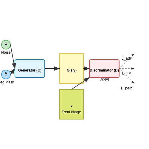
A notable implementation is the pix2pixHD framework adapted for T1-weighted to T2-weighted MRI translation. The generator employs a coarse-to-fine architecture with residual blocks, while the discriminator uses a multi-scale PatchGAN to assess local realism. The loss function combines adversarial loss, feature matching loss, and a perceptual loss derived from a pre-trained VGG network:
where λ terms balance the contributions. This approach achieves a Structural Similarity Index (SSIM) of 0.92 on the BraTS dataset, outperforming non-conditional baselines by 15%.
5. Training Instability and Sensitivity to Conditions
5.1 Training Instability and Sensitivity to Conditions
Conditional GANs inherit the training instability challenges of standard GANs while introducing additional complexities from conditional information. The minimax objective:
becomes more sensitive to conditional input y due to the expanded hypothesis space. Three primary instability mechanisms emerge:
Conditional Mode Collapse
When the generator learns to ignore specific conditions or produces identical outputs for different y, the model suffers from conditional mode collapse. This occurs when:
Empirical studies show this is particularly prevalent when using sparse or imbalanced conditioning vectors. The discriminator's gradient signals may become uninformative for underrepresented conditions.
Conditional Gradient Conflict
The interplay between condition-dependent and unconditional gradients creates conflicting optimization directions. For a generator parameter θ:
compete with the condition-preservation term in many implementations. This manifests as oscillating loss curves where the generator alternates between satisfying conditions and fooling the discriminator.
Spectral Sensitivity
cGANs exhibit heightened sensitivity to the spectral properties of conditioning vectors. Analysis of the Jacobian matrix:
reveals that high condition-space curvature (large singular values) correlates with training divergence. This explains why embedding-based conditions often outperform one-hot encodings in practice.
Stabilization Techniques
Several architectural and optimization approaches mitigate these issues:
- Conditional Batch Normalization: Layer-specific scaling parameters γ(y), β(y) maintain condition sensitivity throughout the network
- Projection Discriminators: Dot-product conditioning preserves gradient coherence
- Gradient Penalty: The condition-aware variant enforces Lipschitz continuity on D(x|y)
Recent work on consistency regularization shows particular promise by enforcing:
through auxiliary loss terms. This maintains the geometric structure of the condition space in the generated outputs.
5.2 Evaluation Metrics for Conditional Generation
Quantitative Metrics for cGAN Performance
Evaluating the performance of conditional generative adversarial networks (cGANs) requires specialized metrics that assess both the quality of generated samples and their alignment with the conditioning input. Unlike unconditional GANs, cGANs must satisfy two criteria: realism (samples should resemble real data) and conditional consistency (samples must match the given condition).
This objective function highlights the dual requirement of cGANs, where D discriminates between real pairs (x,y) and generated pairs (G(z|y), y).
Inception Score (IS) with Conditioning
The standard Inception Score measures sample quality and diversity but must be adapted for conditional generation. The conditional IS evaluates:
where p(c|x) is the class probability predicted by an Inception-v3 network, and p(c|y) is the expected class distribution given condition y. Higher values indicate better conditional alignment.
Frechet Inception Distance (FID) for Conditional Samples
FID compares statistics of real and generated samples in a feature space. For cGANs, we compute separate FID scores per condition:
where μy, Σy are the mean and covariance of real samples for condition y, and μ̃y, Σ̃y are those of generated samples. The final metric averages across conditions.
Conditional Consistency Metrics
These metrics specifically evaluate how well generated samples match their conditions:
Classification Accuracy Score (CAS)
A pre-trained classifier C predicts the condition from generated samples. CAS is the percentage of samples where C(G(z|y)) = y:
Perceptual Path Length (PPL) with Conditions
PPL measures the stability of interpolations in latent space while holding the condition constant. For cGANs, we compute:
where d(·,·) is a perceptual distance metric (e.g., LPIPS), and lerp denotes linear interpolation.
Human Evaluation Protocols
While quantitative metrics are essential, human evaluation remains critical for conditional generation tasks. Common protocols include:
- Two-Alternative Forced Choice (2AFC): Evaluators choose between real and generated samples for a given condition.
- Condition Matching Tests: Evaluators identify which of multiple conditions matches a generated sample.
- Mean Opinion Score (MOS): Rated on scales for realism, condition alignment, and overall quality.
Domain-Specific Metrics
Certain applications require specialized metrics:
- Image-to-Image Translation: SSIM, PSNR, and segmentation accuracy between input and output.
- Text-to-Image Generation: R-precision (retrieval accuracy of text descriptions from generated images).
- Audio Generation: Mel-cepstral distortion (MCD) for voice conversion tasks.
5.3 Ethical Considerations and Bias in cGANs
Sources of Bias in cGANs
Conditional GANs inherit biases from their training data, which can propagate or amplify societal prejudices. The generator G learns the joint distribution P(X, Y) where X is the data and Y is the conditioning variable. If the training dataset contains imbalanced representations across classes (e.g., gender, race, or age), the model will reproduce these biases in generated samples. Mathematically, this occurs because the generator minimizes the Jensen-Shannon divergence:
When pdata(x|y) is skewed for certain values of y, the generator G(z|y) will replicate this skewness. For example, if a cGAN trained on facial images has underrepresentation of darker skin tones in the training set, generated images will exhibit the same underrepresentation.
Amplification of Stereotypes
cGANs can inadvertently reinforce harmful stereotypes. A study by Buolamwini and Gebru (2018) demonstrated that facial recognition systems trained on biased datasets perform poorly on underrepresented groups. Similarly, a cGAN conditioned on occupation labels might generate predominantly male images for "CEO" or "engineer" if the training data reflects historical gender imbalances. This occurs because the discriminator D is trained to classify real vs. fake samples based on the empirical distribution, which may encode societal biases.
Privacy and Consent Issues
cGANs trained on sensitive data (e.g., medical images or personal photos) raise privacy concerns. Even if the generated samples are synthetic, they may retain identifiable features from the training data. The risk is particularly high when conditioning on rare or unique attributes, as the generator may inadvertently reproduce near-copies of training examples. Differential privacy techniques, such as adding noise to gradients during training, can mitigate this:
where σ controls the privacy-utility trade-off.
Mitigation Strategies
- Dataset Auditing: Preprocess training data to ensure balanced representation across conditioning variables. Tools like IBM's AI Fairness 360 can detect imbalances.
- Adversarial Debiasing: Train an auxiliary classifier to penalize the generator for producing biased outputs. The loss function becomes:
where C is a fairness classifier and λ controls the debiasing strength.
- Post-hoc Correction: Apply resampling or rejection sampling to generated outputs to enforce demographic parity.
Case Study: Bias in Medical cGANs
A 2021 study found that cGANs trained on chest X-rays exhibited racial bias in generated images, with lower accuracy for Black patients due to dataset imbalances. The model's FID score (Fréchet Inception Distance) was 15% higher for underrepresented groups, indicating poorer quality generation. This highlights the critical need for bias audits in healthcare applications.
6. Key Research Papers on cGANs
6.1 Key Research Papers on cGANs
- [1411.1784] Conditional Generative Adversarial Nets - arXiv.org — Generative Adversarial Nets [8] were recently introduced as a novel way to train generative models. In this work we introduce the conditional version of generative adversarial nets, which can be constructed by simply feeding the data, y, we wish to condition on to both the generator and discriminator. We show that this model can generate MNIST digits conditioned on class labels. We also ...
- RoCGAN: Robust Conditional GAN | International Journal of ... - Springer — Conditional image generation lies at the heart of computer vision and conditional generative adversarial networks (cGAN) have recently become the method of choice for this task, owing to their superior performance. The focus so far has largely been on performance improvement, with little effort in making cGANs more robust to noise. However, the regression (of the generator) might lead to ...
- Conditional GANs (CGANs) with codes explained - Medium — In short, CGANs differ from Vanilla GANs only in the point that we are passing label information to both the generator and discriminator, and the generation process is guided by this meta information.
- How to Develop a Conditional GAN (cGAN) From Scratch — In the paper, the authors motivate the approach based on the desire to direct the image generation process of the generator model. ... Although GANs can be conditioned on the class label, so-called class-conditional GANs, they can also be conditioned on other inputs, such as an image, in the case where a GAN is used for image-to-image ...
- Image-to-Image Translation with Conditional Adversarial Networks - ar5iv — GANs have been vigorously studied in the last two years and many of the techniques we explore in this paper have been previously proposed. Nonetheless, earlier papers have focused on specific applications, and it has remained unclear how effective image-conditional GANs can be as a general-purpose solution for image-to-image translation.
- A survey on GANs for computer vision: Recent research, analysis and ... — Neural networks can be used as a C2ST, as mentioned in previous sections, D is indeed a classifier of real and generated data. As is proposed in [65], a C2ST can be applied to GANs by using the same composition of the discriminator, as is said in the paper "training a fresh discriminator on a fresh set of data". C2ST-Neural Network (C2ST-NN).
- A Review on Generative Adversarial Networks: Algorithms, Theory, and ... — Generative adversarial networks (GANs) have recently become a hot research topic; however, they have been studied since 2014, and a large number of algorithms have been proposed. Nevertheless, few comprehensive studies explain the connections among different GAN variants and how they have evolved. In this paper, we attempt to provide a review of the various GAN methods from the perspectives of ...
- Conditional Generative Adversarial Networks with Optimized Machine ... — In recent years, digital twin (DT) technology has garnered significant interest from both academia and industry. However, the development of effective fault detection and diagnosis models remains challenging due to the lack of comprehensive datasets. To address this issue, we propose the use of Generative Adversarial Networks (GANs) to generate synthetic data that replicate real-world data ...
- Interpreting CNN predictions using conditional Generative Adversarial ... — A Generative Adversarial Network (GAN) [17] is an unsupervised neural network used for generating unstructured data, such as synthetic images. It is composed of two parts, namely a generator and a discriminator. The generator uses a latent space to build a synthetic image, and the discriminator is trained to recognize the difference between a real and a synthetic image.
- (PDF) Generative Adversarial Networks (GANs): An Overview of ... — In this paper, after introducing the main concepts and the theory of GAN, two new deep generative models are compared, the evaluation metrics utilized in the literature and challenges of GANs are ...
6.2 Recommended Books and Tutorials
- Generative AI 6: Advanced GAN Techniques - TechBlog By Dhiraj — These techniques make GANs more powerful and adaptable for real-world applications, especially in generating high-quality images, videos, and other data. 6.1 Conditional GANs (cGANs) What are Conditional GANs (cGANs)? Conditional GANs (cGANs) extend the basic GAN architecture by conditioning both the generator and discriminator on additional ...
- 9 Books on Generative Adversarial Networks (GANs) — Discover how to develop DCGANs, conditional GANs, Pix2Pix, CycleGANs, and more with Keras in my new GANs book, with 29 step-by-step tutorials and full source code. Let's get started. GAN Books. Most of the books have been written and released under the Packt publishing company.
- conditional-gans-cgans-explained.md - GitHub — Conditional Generative Adversarial Networks, or cGANs for short, improve regular or 'vanilla' GANs by adding a condition into the Generator and Discriminator networks. The idea is that it allows a GAN to better structure its latent space and the mapping into data space, and the concept of a cGAN was proposed by Mirza & Osindero (2014).
- What Are Conditional Generative Adversarial Networks (cGANs)? - Coursera — Controlled data generation: cGANs allow for data generation that meets specific conditions, allowing you to give details related to the type of output you are looking for. Enhances capabilities of standard GANs: By introducing conditions, cGANs expand the capabilities of GANs, offering more precision and relevance in the data generated. Cons
- Conditional Generative Adversarial Network - GeeksforGeeks — In the next step we need to define the Loss function and optimizer for the discriminator and generator networks in a Conditional Generative Adversarial Network(CGANS). Binary Cross-Entropy Loss (bce loss) is suitable for distinguishing between real and fake data in GANs. The discriminator loss function take two arguments, real and fake.
- Chapter 8. Conditional GAN · GANs in Action: Deep learning with ... — Using labels to train both the Generator and the Discriminator · Teaching GANs to generate examples matching a specified label · Implementing a Conditional GAN (CGAN) to generate handwritten digits of our choice ... In the remainder of this chapter, you will learn how CGANs work and implement a small-scale version by using (you guessed it ...
- Conditional GANs - Python Deep Learning - Second Edition [Book] — Conditional GANs. Conditional GANs (CGANs) are an extension of the GAN framework where both the generator and discriminator receive some additional conditioning input information,.This could be the class of the current image or some other property.. For example, if we train a GAN to generate new MNIST images, we could add an additional input layer with values of one-hot-encoded image labels:
- Conditional GANs (CGANs) with codes explained - Medium — Conditional GANs do the exact thing !! They intake input from the user about which class they wish to generate an image for and they generate an image belonging to the same class. Voila!!
- Generative Adversarial Networks (GANs) - IEEE Xplore — By covering the principles of GANs, it looks at such early GANs and shows how to obtain satisfactory training. The chapter focuses on two well‐known generative models, namely deep convolutional GAN and conditional GAN (CGAN). CGAN for simplicity, is a type of GAN that involves the conditional generation of data instances by a generator model.
- 9 Books on Generative Adversarial Networks (GANs) — Generative Adversarial Networks, or GANs for short, were first described in the 2014 paper by Ian Goodfellow, et al. titled "Generative Adversarial Networks." Since then, GANs have seen a lot of attention given that they are perhaps one of the most effective techniques for generating large, high-quality synthetic images. As such, a number of books […]
6.3 Open-Source Implementations and Datasets
- GitHub - weiyueli7/cGANs-cDCGANs: Implementations of Conditional GANs ... — By leveraging the capabilities of generative adversarial networks (GANs) and incorporating conditional inputs, the proposed approach enables the generation of images with specific desired attributes. The project involves training cDCGANs and cGANs on large-scale labeled datasets, where the models are conditioned on auxiliary information such as ...
- Conditional GANs (cGANs) explained | MachineCurve.com — Conditional Generative Adversarial Networks, or cGANs for short, improve regular or 'vanilla' GANs by adding a condition into the Generator and Discriminator networks. The idea is that it allows a GAN to better structure its latent space and the mapping into data space, and the concept of a cGAN was proposed by Mirza & Osindero (2014).
- Generative adversarial networks for medical image synthesis — Various networks and architectures have been proposed for better performance on different tasks. In this literature survey, a class of network architectures, called generative adversarial networks (GANs), especially the conditional GANs (cGANs) [44] and cycle-consistent GANs (Cycle-GANs), are introduced and explained. The emerging GAN-based ...
- Conditional GANs (CGANs) with codes explained - Medium — In short, CGANs differ from Vanilla GANs only in the point that we are passing label information to both the generator and discriminator, and the generation process is guided by this meta information.
- GAN Compression: Efficient Architectures for Interactive Conditional GANs — Conditional Generative Adversarial Networks (cGANs) have enabled controllable image synthesis for many vision and graphics applications. However, recent cGANs are 1-2 orders of magnitude more compute-intensive than modern recognition CNNs. For example, GauGAN consumes 281G MACs per image, compared to 0.44G MACs for MobileNet-v3, making it difficult for interactive deployment. In this work, we ...
- Lecture 6 Implicit Models -- Generative Adversarial Networks (GANs ... — 6 Creative Conditional GANs. Introduced in 2014 by University of Montreal PhD student Mehdi Mirza and Flickr AI architect Simon Osindero, Conditional GAN is a generative adversarial network whose Generator and Discriminator are conditioned during training by using some addi- tional information Conditional GAN (cGAN) allows us to condition the network with additional information such as class ...
- CcGAN: Continuous Conditional Generative Adversarial Networks for... — This work proposes the continuous conditional generative adversarial network (CcGAN), the first generative model for image generation conditional on continuous, scalar conditions (termed regression labels). Existing conditional GANs (cGANs) are mainly designed for categorical conditions (e.g., class labels); conditioning on a continuous label is mathematically distinct and raises two ...
- [Project] PyTorch Implementations of 37 GAN papers (including ... - Reddit — Extensive GAN implementations using PyTorch. The only repository to train/evaluate BigGAN and StyleGAN2 baselines in a unified training pipeline. Comprehensive benchmark of GANs using CIFAR10, Tiny ImageNet, CUB200, and ImageNet datasets. Provide pre-trained models that are fully compatible with up-to-date PyTorch environment.
- [Hands-On] Understanding and Implementing Conditional GAN — Conditional Information: Additional information received by both the generator and the discriminator. For example, in the MNIST dataset, the digits from 0 to 9 are used as conditional information.
- GitHub - Lornatang/conditional_gan: Simple implementation of ... — If you're new to CGANs, here's an abstract straight from the paper: Generative Adversarial Nets were recently introduced as a novel way to train generative models. In this work we introduce the conditional version of generative adversarial nets, which can be constructed by simply feeding the data, y, we wish to condition on to both the ...