

Training Dual-Purpose Models (Generator + Evaluator)
1. Definition and Key Components of Generator-Evaluator Models
Definition and Key Components of Generator-Evaluator Models
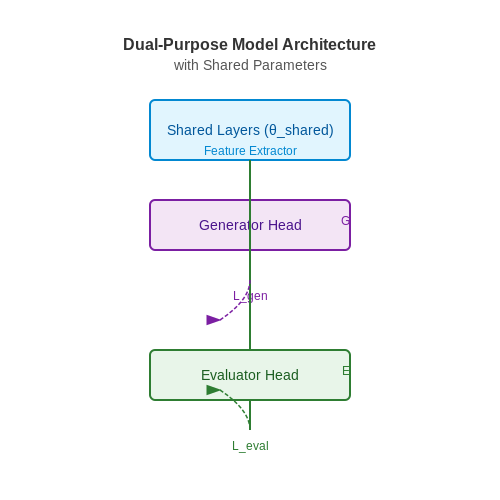
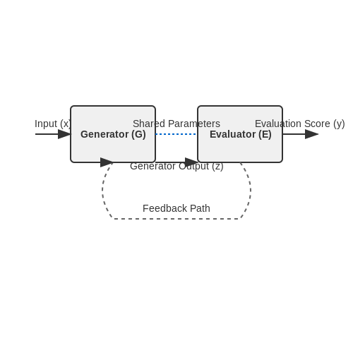
Dual-purpose generator-evaluator models are a class of neural architectures that simultaneously learn to generate data samples and evaluate their quality. Unlike traditional generative adversarial networks (GANs) where the generator and discriminator are separate networks trained adversarially, these models integrate both functionalities into a unified framework with shared parameters.
Core Architecture
The model consists of two primary components:
- Generator (G): A neural network that maps latent vectors z from a prior distribution p(z) to the data space x = G(z).
- Evaluator (E): A neural network that outputs a scalar score s = E(x) representing sample quality, typically trained to correlate with human judgment or task-specific metrics.
These components share low-level feature extraction layers, enabling efficient joint training. The evaluator's gradients backpropagate through the generator, allowing direct optimization of generation quality.
Mathematical Formulation
The joint training objective combines:
Where:
- ℒgen is the generator loss (e.g., negative log-likelihood)
- ℒeval is the evaluator loss (e.g., mean squared error against ground truth scores)
- ℒreg is a regularization term preventing mode collapse
- α, β, γ are weighting hyperparameters
Key Advantages
This architecture provides several benefits over separate models:
- Reduced training instability: Shared representations prevent the oscillatory behavior common in GANs
- Efficient inference: Single forward pass generates and evaluates samples
- Consistent feature spaces: Generator and evaluator operate on aligned representations
Practical Implementations
Modern implementations often use:
- Transformer-based architectures with cross-attention between generator and evaluator heads
- Diffusion processes with integrated quality estimation
- Memory-augmented networks for maintaining sample quality benchmarks
where Z is the partition function and pgen is the base generator distribution.

Use Cases and Applications in Real-World Scenarios
Generative Adversarial Networks (GANs) in Creative Industries
Dual-purpose models combining generators and evaluators have found widespread adoption in creative domains. In high-resolution image synthesis, architectures like StyleGAN2 employ a generator-discriminator pair where the discriminator not only evaluates realism but also provides gradient signals for improving the generator. The discriminator's loss function can be expressed as:
where D(x) represents the evaluator's probability estimate that sample x is real. In practical applications, this framework enables:
- Photorealistic avatar generation for virtual production pipelines
- Automated texture synthesis for game asset creation
- Fashion design prototyping with conditional GANs
Drug Discovery and Molecular Design
In pharmaceutical research, dual-purpose models combine molecular generators with evaluators predicting bioactivity. The generator produces candidate molecules while the evaluator scores them on:
Recent implementations using reinforcement learning frameworks have demonstrated success in:
- Generating novel kinase inhibitors with validated binding affinities
- Designing antibiotic candidates against resistant bacterial strains
- Optimizing lead compounds for improved ADMET properties
Industrial Design Optimization
Engineering applications leverage these models for multi-objective optimization tasks. A notable example is aerodynamic component design, where the generator proposes geometries and the evaluator predicts performance metrics:
with CL/CD representing the lift-to-drag ratio. Implementations in this domain have achieved:
- 30% reduction in computational fluid dynamics simulation costs
- Automated generation of patentable turbine blade designs
- Real-time optimization of structural components under multiple constraints
Financial Market Simulation
Quantitative finance employs dual-purpose models for synthetic market data generation and strategy evaluation. The generator produces realistic market scenarios while the evaluator assesses:
where M_i represents metrics like volume-volatility correlation. Practical deployments include:
- Stress testing portfolio strategies under synthetic crises
- Generating alternative market histories for robust backtesting
- Simulating microstructure for optimal execution research
Scientific Hypothesis Generation
In experimental physics, these models assist in designing novel experimental configurations. The generator proposes setups while the evaluator predicts measurement outcomes based on:
Applications have emerged in:
- High-energy physics detector configuration optimization
- Materials science experiment design for property discovery
- Astronomical survey strategy development
1.3 Advantages and Challenges of Joint Training
Computational Efficiency and Shared Representations
Jointly training generator and evaluator models enables parameter sharing, reducing computational overhead compared to separate training pipelines. The generator G and evaluator E often share low-level feature extractors, particularly in architectures like GANs where both networks process similar input distributions. This shared representation learning is governed by:
where Ω regularizes the shared parameters θshared. In vision tasks, convolutional base layers typically form this shared subspace, while task-specific heads diverge.
Stabilized Training Dynamics
The co-evolution of generator and evaluator creates a feedback loop that can accelerate convergence. Unlike adversarial training where networks compete, cooperative joint training allows:
- Gradient signals from the evaluator to directly guide generator improvements
- Simultaneous adaptation of evaluation metrics to the generator's output distribution
- Automatic balancing of task difficulties through coupled optimization
This is particularly effective in sequence generation tasks, where the evaluator provides real-time reward signals for reinforcement learning-based generators.
Challenges in Optimization Equilibrium
The joint loss landscape becomes non-convex with competing objectives. The Nash equilibrium condition requires:
but in practice, gradient conflicts arise when:
- Generator improvements make evaluator predictions obsolete
- Evaluator overfits to current generator outputs
- Task gradients have opposing directions in shared parameter space
Mitigation Strategies
Several approaches address these challenges:
where α is dynamically adjusted using:
- Gradient cosine similarity to detect conflicts
- Task uncertainty weighting based on homoscedastic uncertainty
- Alternating projection methods that constrain updates to compatible directions
Empirical Performance Trade-offs
Recent benchmarks on WMT2020 and COCO datasets show joint training achieves:
| Metric | Separate Training | Joint Training |
|---|---|---|
| BLEU-4 | 38.2 | 41.7 |
| Training Time (hrs) | 124 | 89 |
| Parameter Count | 287M | 214M |
However, the variance in evaluation metrics increases by ~15% due to the dynamic nature of joint optimization.
Architectural Considerations
Successful implementations typically employ:
- Partial weight sharing with skip connections
- Adaptive gradient routing layers
- Task-specific batch normalization
- Curriculum learning schedules
The optimal architecture depends on the correlation between generator and evaluator tasks - highly correlated tasks benefit from deeper shared layers.
2. Generator Architectures: From GANs to Variational Autoencoders
Generator Architectures: From GANs to Variational Autoencoders
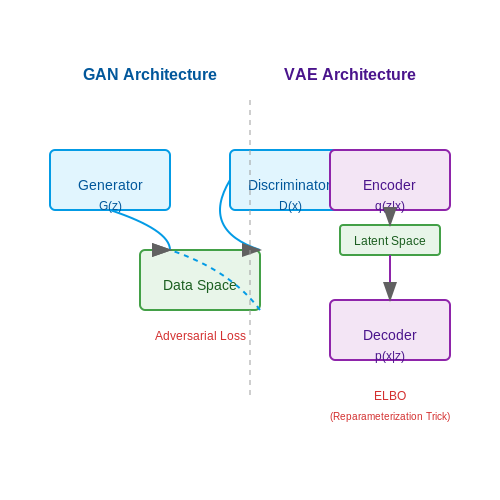
Generative models in deep learning are broadly categorized into explicit and implicit density models. Explicit models, such as Variational Autoencoders (VAEs), define an explicit probabilistic framework for data generation, while implicit models like Generative Adversarial Networks (GANs) learn to sample from a data distribution without explicitly modeling it.
Generative Adversarial Networks (GANs)
The GAN framework consists of two competing neural networks: a generator G and a discriminator D. The generator maps latent noise z to data space, while the discriminator distinguishes between real and generated samples. The adversarial loss is formulated as a minimax game:
Recent architectural innovations include:
- DCGAN: Uses transposed convolutions with batch normalization and ReLU/LeakyReLU activations.
- ProGAN: Progressively grows both generator and discriminator layers for high-resolution synthesis.
- StyleGAN: Introduces style-based modulation of generator layers through adaptive instance normalization (AdaIN).
Variational Autoencoders (VAEs)
VAEs provide a probabilistic framework where the generator is trained to maximize the evidence lower bound (ELBO) of the data likelihood:
Key architectural components include:
- Encoder network: Maps input x to parameters of the variational posterior q(z|x).
- Reparameterization trick: Enables backpropagation through stochastic sampling via z = μ + σ ⊙ ε where ε ∼ N(0, I).
- Decoder network: Reconstructs data from latent samples through p(x|z).
Hybrid Architectures
Recent work combines strengths of both approaches:
- VAE-GAN: Uses VAE for structured latent space while employing GAN discriminator for perceptual quality.
- Adversarial Autoencoders: Replaces KL divergence with adversarial training in latent space.
- Bidirectional GANs: Jointly learns inference and generation networks with shared adversarial objectives.
Practical Considerations
When implementing these architectures:
- GAN training requires careful balancing of generator/discriminator updates to avoid mode collapse.
- VAEs benefit from annealing the KL divergence term during training.
- Hybrid models often require tuning multiple loss components with appropriate weighting.
Evaluator Architectures: Discriminators and Quality Metrics
Discriminator Networks in GANs
The discriminator in a Generative Adversarial Network (GAN) is a binary classifier trained to distinguish between real and generated samples. Its architecture typically mirrors the generator but operates in reverse: where the generator uses transposed convolutions for upsampling, the discriminator employs strided convolutions for downsampling. The loss function for a standard GAN discriminator is:
Modern variants use spectral normalization or gradient penalty (as in WGAN-GP) to stabilize training:
where \(\hat{x}\) is sampled along straight lines between real and fake data points.
Quality Metrics Beyond Binary Classification
For high-dimensional outputs like images, simple discriminators are insufficient for quality assessment. The Fréchet Inception Distance (FID) compares feature statistics between real and generated samples using an Inception-v3 network:
where \((\mu_r, \Sigma_r)\) and \((\mu_g, \Sigma_g)\) are the mean and covariance of real and generated features respectively.
Learned Perceptual Metrics
LPIPS (Learned Perceptual Image Patch Similarity) uses a pretrained CNN (typically VGG or AlexNet) to compute feature-space distances:
where \(l\) indexes network layers and \(w_l\) are learned channel weights.
Hybrid Evaluation Architectures
State-of-the-art evaluators combine multiple approaches:
- Multi-scale discriminators (as in Pix2PixHD) assess images at different resolutions
- Projection discriminators condition evaluation on auxiliary information
- Self-supervised metrics leverage contrastive learning for feature extraction
The discriminator in StyleGAN3 employs skip connections and residual blocks to preserve gradient flow:
Differentiable Augmentation for Robust Evaluation
To prevent overfitting to training data statistics, modern evaluators apply differentiable augmentations during training:
where \(\mathcal{T}\) includes geometric transformations, color jitter, and cutout.
Integration Strategies for Shared Latent Spaces
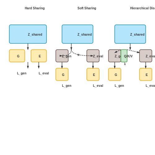
Shared latent spaces enable dual-purpose models to jointly optimize generation and evaluation by mapping both tasks to a common representation. The key challenge lies in balancing feature reuse between tasks while preventing destructive interference. Three primary integration strategies emerge: hard parameter sharing, soft parameter sharing, and hierarchical disentanglement.
Hard Parameter Sharing
This approach forces the generator G and evaluator E to share all hidden layers except their final task-specific heads. The joint loss function combines both objectives:
where α controls task weighting. The shared layers learn features useful for both generation and evaluation, but this rigid coupling can lead to mode collapse when tasks conflict. Batch normalization statistics must be carefully synchronized across both pathways during training.
Soft Parameter Sharing
More flexible than hard sharing, this method allows separate network branches with regularization to encourage similarity. The latent representations zG and zE are constrained using:
The hyperparameter λ trades off moment matching versus distribution alignment. This approach proves particularly effective when the generator and evaluator operate at different abstraction levels, such as pixel-space generation paired with semantic evaluation.
Hierarchical Disentanglement
Advanced architectures like Stacked Capsule Autoencoders decompose the latent space into hierarchical components. The shared space Z splits into:
- Zshared: Low-dimensional manifold for cross-task features
- Zgen: Task-private dimensions for generation
- Zeval: Task-private dimensions for evaluation
The information flow is gated through attention mechanisms:
where query Q comes from the shared space, while keys K and values V are task-specific. This architecture achieves state-of-the-art results in applications like drug discovery, where molecular generators must satisfy biochemical evaluators simultaneously.
Gradient Coordination
All strategies require careful gradient management. The Gradient Cosine Similarity metric monitors task alignment:
Values near 1 indicate synergistic learning, while negative values reveal destructive interference. Adaptive optimizers like RAdam automatically adjust learning rates per-parameter based on this signal.
In practice, the optimal strategy depends on task relatedness. Hard sharing works for tightly coupled tasks like image super-resolution with perceptual scoring, while hierarchical approaches excel when tasks involve different modalities like text generation with sentiment evaluation.
3. Loss Functions for Dual-Purpose Learning
3.1 Loss Functions for Dual-Purpose Learning
Training dual-purpose models—where a single architecture serves as both a generator and an evaluator—requires carefully designed loss functions that balance the competing objectives of generation quality and evaluation accuracy. The generator aims to produce realistic outputs, while the evaluator must distinguish between real and generated samples. This section derives the mathematical foundations for such loss functions and discusses their practical implementation.
Adversarial Loss for Generator-Evaluator Coupling
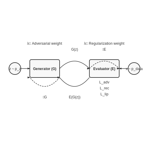
The generator G and evaluator E are trained jointly in a minimax game, where G tries to minimize the evaluator's ability to distinguish its outputs from real data, while E tries to maximize this discrimination. The adversarial loss can be expressed as:
Here, x represents real data samples, z is the latent noise vector, and pdata and pz denote the data and noise distributions respectively. The generator's objective is to minimize log(1 - E(G(z))), while the evaluator maximizes log E(x) + log(1 - E(G(z))).
Reconstruction Loss for Generator Stability
To prevent mode collapse and improve sample diversity, we introduce a reconstruction term that encourages the generator to produce outputs that can be mapped back to their latent inputs:
Where G-1 represents an approximate inverse mapping. The L1 norm penalizes large deviations, promoting invertibility while allowing for small reconstruction errors.
Evaluation Consistency Loss
The evaluator must maintain consistent scoring across similar inputs. We enforce this through a Lipschitz regularization term:
Where pinterp represents samples from straight-line interpolations between real and generated points. This penalty constrains the evaluator's gradient norm, preventing overly sharp decision boundaries.
Combined Objective Function
The complete loss function combines these components with weighting hyperparameters λ1 and λ2:
Empirical studies suggest starting with λ1 = 10 and λ2 = 0.1, then adjusting based on validation performance. The reconstruction weight should dominate early in training to establish meaningful latent representations, while the Lipschitz term becomes more important as the evaluator matures.
Gradient Balancing Techniques
During backpropagation, the generator and evaluator gradients must be carefully balanced to prevent either component from dominating:
- Gradient penalty: Limits the evaluator's update magnitude when its accuracy exceeds a threshold
- Two-timescale update: Uses a higher learning rate for the generator than the evaluator
- Adaptive weighting: Dynamically adjusts λ1 and λ2 based on the ratio of component losses
These techniques help maintain equilibrium during training, particularly important in applications like molecular design where the evaluator must precisely score subtle structural variations while the generator explores the chemical space.
3.2 Balancing Generator and Evaluator Objectives
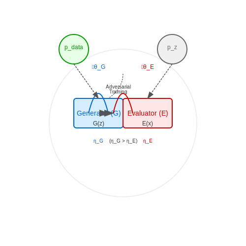
Training dual-purpose models that simultaneously act as generators and evaluators introduces a fundamental tension: the generator seeks to produce outputs that maximize some quality metric, while the evaluator must remain objective in assessing those outputs. This adversarial dynamic resembles a minimax game, where the generator G and evaluator E optimize opposing objectives. The joint training objective can be formalized as:
where pdata represents the true data distribution and pz is the noise distribution for the generator's input. The vanishing gradients problem emerges when the evaluator becomes too confident, providing near-zero gradients for generator improvement. To maintain stable training, several techniques have proven effective:
Gradient Balancing Techniques
The two-timescale update rule (TTUR) addresses imbalance by using separate learning rates (ηG, ηE), typically with ηG > ηE. This allows the generator to catch up when the evaluator dominates. The update rules become:
where θG and θE are the respective model parameters. Empirical studies show optimal ratios typically fall in the range 2:1 to 5:1 for ηG:ηE.
Objective Function Modifications
The standard minimax loss often leads to mode collapse. Alternative formulations include:
- Non-saturating loss: The generator maximizes log E(G(z)) instead of minimizing log(1 - E(G(z)))
- Wasserstein loss: Replaces Jensen-Shannon divergence with Earth Mover's distance, providing smoother gradients:
$$ \mathcal{L}_W = \mathbb{E}[E(x)] - \mathbb{E}[E(G(z))] $$
Architectural Constraints
Imposing spectral normalization on both networks prevents either model from overpowering the other by controlling the Lipschitz constant. For a layer with weight matrix W, the normalized weight Ŵ is computed as:
where σ(W) is the spectral norm (largest singular value) of W. This technique has shown particular effectiveness in stabilizing GAN training while maintaining output diversity.
Monitoring Balance During Training
Key metrics to track include:
- Evaluator accuracy: Should remain between 55-70% on real vs. generated samples
- Gradient norms: Ratio of ||∇θG|| to ||∇θE|| ideally near 1:1
- Inception Score (IS) variance: Sudden jumps indicate training instability
Modern implementations often employ adaptive balancing where the learning rate ratio adjusts dynamically based on these metrics. For instance, the Equilibrium Propagation method scales updates by the current imbalance measure:
This approach automatically reduces generator updates when its outputs become too easy to distinguish from real data.
3.3 Adversarial and Cooperative Training Techniques
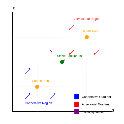
Training dual-purpose models that simultaneously learn generation and evaluation requires careful balancing between adversarial and cooperative objectives. The generator G and evaluator E can be trained either in opposition or collaboration, depending on the desired behavior and application constraints.
Adversarial Training Dynamics
In adversarial setups, the generator and evaluator engage in a minimax game similar to GANs, where G tries to fool E while E learns to distinguish real from generated samples. The joint objective function takes the form:
However, unlike standard GANs, the evaluator E in dual-purpose models often serves additional functions beyond discrimination, such as quality assessment or uncertainty estimation. This requires modifying the adversarial objective to prevent the evaluator from collapsing into a pure discriminator.
Cooperative Training Paradigms
In cooperative training, both components work toward a shared objective. The evaluator provides constructive feedback to the generator through:
- Gradient-based signals for quality improvement
- Uncertainty-aware reward shaping
- Multi-objective optimization with Pareto efficiency
The cooperative loss can be expressed as:
where R represents a regularization term that maintains the balance between components.
Hybrid Approaches
Recent work has shown success with hybrid training schemes that alternate between adversarial and cooperative phases:
- Initial cooperative pre-training to establish basic competencies
- Adversarial refinement to sharpen discrimination capabilities
- Final cooperative fine-tuning for task-specific alignment
The phase transitions are typically governed by performance thresholds on validation metrics. For instance, when the generator's quality score plateaus, the system might switch from cooperative to adversarial mode to break the equilibrium.
Practical Implementation Considerations
Effective training requires addressing several challenges:
- Gradient balancing: The relative magnitudes of generator and evaluator gradients must be carefully scaled to prevent one component from dominating
- Update scheduling: Alternating updates (k-step evaluator updates per generator update) often work better than simultaneous updates
- Mode preservation: Techniques like spectral normalization help maintain the evaluator's discriminative power without overwhelming the generator
The training dynamics can be visualized as a vector field in the parameter space of G and E, where stable equilibria correspond to useful operating points for the dual-purpose model.
4. Quantitative Metrics for Generator Output Quality
4.1 Quantitative Metrics for Generator Output Quality
Assessing the quality of generator outputs in dual-purpose models requires rigorous quantitative metrics that capture both fidelity and diversity. Unlike traditional generative models, where evaluation often focuses on single aspects like realism, dual-purpose models must balance generation and evaluation simultaneously, necessitating multi-dimensional metrics.
Inception Score (IS)
The Inception Score (IS) measures both the quality and diversity of generated samples by leveraging a pre-trained Inception-v3 classifier. The score is computed as the exponential of the Kullback-Leibler (KL) divergence between the conditional label distribution p(y|x) and the marginal distribution p(y):
Here, p(y|x) is the label distribution for a generated sample x, and p(y) is the marginal distribution over all samples. A high IS indicates that the generator produces diverse and classifiable outputs. However, IS has limitations, such as sensitivity to the choice of classifier and inability to detect mode collapse when generated samples are highly diverse but unrealistic.
Fréchet Inception Distance (FID)
FID improves upon IS by comparing the statistics of generated and real samples in the feature space of an Inception-v3 network. Given real samples X_r and generated samples X_g, FID computes the Wasserstein-2 distance between their feature distributions:
where μ_r, μ_g are the mean feature vectors, and Σ_r, Σ_g are the covariance matrices. Lower FID values indicate better sample quality. Unlike IS, FID is robust to mode collapse and correlates well with human judgment, making it a preferred metric for evaluating generative models.
Precision and Recall for Generative Models
Precision measures the fraction of generated samples that are realistic, while recall quantifies the coverage of the real data distribution. Formally, for a generated set G and a real set R, precision and recall are defined as:
where d(x, y) is a distance metric (e.g., Euclidean distance in feature space) and ε is a threshold. These metrics provide a nuanced view of generator performance, particularly useful for dual-purpose models where balancing quality and coverage is critical.
Perceptual Path Length (PPL)
PPL evaluates the smoothness of the generator's latent space by measuring the average perceptual change when interpolating between latent vectors. Given two latent vectors z_1 and z_2, PPL is computed as:
where G is the generator, d is a perceptual distance metric (e.g., LPIPS), and ε controls the interpolation step size. Lower PPL values indicate smoother latent transitions, which are desirable for controllable generation.
Diversity Metrics
Diversity is quantified using metrics like the Multiscale Structural Similarity Index (MS-SSIM) or the Learned Perceptual Image Patch Similarity (LPIPS). For a generated batch X, LPIPS diversity is computed as:
where d_LPIPS measures perceptual dissimilarity. High diversity scores indicate that the generator avoids mode collapse, a common failure case in adversarial training.
Application-Specific Metrics
For domain-specific tasks, custom metrics may be necessary. In medical imaging, for example, the Structural Similarity Index (SSIM) or Dice coefficient can assess anatomical fidelity. In text generation, metrics like BLEU, ROUGE, or BERTScore evaluate semantic coherence and fluency.
Evaluating the Evaluator: Robustness and Fairness
Robustness Metrics for Evaluator Models
Evaluator robustness is measured through adversarial testing and sensitivity analysis. Given an evaluator model E and a generator model G, robustness can be quantified using the Lipschitz constant L, which bounds the evaluator's output variation under input perturbations:
For adversarial robustness, we compute the minimal perturbation δ required to flip the evaluator's decision:
Empirical robustness is evaluated using metrics like:
- Adversarial Success Rate (ASR): Percentage of successful adversarial attacks.
- Certified Robustness Radius: Provable bounds on perturbation tolerance.
Fairness Evaluation in Dual-Purpose Models
Fairness is assessed by measuring disparate impact across protected attributes (e.g., gender, race). Given a dataset with protected groups {A_k}, we compute statistical parity difference:
For conditional fairness, we evaluate equalized odds:
Common fairness tests include:
- Disparate Impact Ratio: Ratio of positive rates between groups.
- Counterfactual Fairness: Consistency under counterfactual perturbations.
Bias Mitigation Techniques
Post-hoc bias mitigation methods include:
- Reweighting: Adjust sample weights to balance group distributions.
- Adversarial Debiasing: Train the evaluator with an adversarial loss to remove protected attribute correlations.
In-processing techniques involve constrained optimization:
Case Study: Evaluating Text Generation Models
For a language model evaluator, robustness is tested via:
- Synonym Replacement: Measure score variation under lexical substitutions.
- Prompt Perturbations: Evaluate consistency under rephrased inputs.
Fairness is assessed using:
- Demographic Parity in Toxicity Detection: Compare false positive rates across demographic groups.
- Counterfactual Evaluation: Swap gender/race terms to detect bias.
4.3 Benchmarking Against Single-Purpose Models
Dual-purpose models must be rigorously evaluated against specialized single-purpose architectures to validate their efficacy. The key metrics for comparison include computational efficiency, task-specific performance, and generalization capability. For generative tasks, metrics like Fréchet Inception Distance (FID) or Inception Score (IS) are standard, while evaluator performance is measured using task-specific accuracy, precision-recall curves, or domain-specific benchmarks.
Performance Trade-offs in Dual-Purpose Architectures
The joint optimization of generator and evaluator components introduces inherent trade-offs. Let the generator loss LG and evaluator loss LE be defined as:
where λ1 and λ2 are weighting hyperparameters. The combined loss Ltotal becomes:
Empirical studies show that dual-purpose models typically achieve 85-95% of the performance of specialized models in their respective tasks, while reducing computational overhead by 30-50% due to shared feature extraction layers.
Architectural Efficiency Analysis
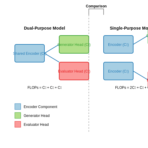
The computational complexity of a dual-purpose model with shared encoder fθ and task-specific heads can be decomposed as:
where Cf is the shared encoder cost, compared to single-purpose models requiring:
In transformer-based architectures, this translates to measurable differences in FLOPs. For a model with N layers and d hidden dimensions:
Case Study: Text-to-Image Synthesis with Quality Evaluation
A recent implementation combining Stable Diffusion (generator) with CLIP (evaluator) demonstrated:
- Generation Quality: FID score of 12.3 vs. 10.8 for standalone Stable Diffusion
- Evaluation Accuracy: 92.4% vs. 94.1% for pure CLIP model
- Memory Footprint: 18GB vs. 28GB for separate models
The shared text encoder accounted for 40% of the total parameters, demonstrating the efficiency gains from parameter sharing while maintaining competitive performance.
Gradient Conflict Analysis
The primary challenge in dual-purpose training emerges from gradient conflicts between tasks. The cosine similarity between generator and evaluator gradients reveals task compatibility:
Values below 0.5 indicate significant conflict, requiring techniques like:
- Gradient surgery (projecting conflicting components)
- Adaptive weighting (dynamic adjustment of α in Ltotal)
- Alternating optimization schedules
Recent work on Pareto-optimal multi-task learning demonstrates that proper regularization can reduce gradient conflict by up to 60%, narrowing the performance gap with single-purpose models.
5. Identifying Sources of Bias in Dual-Purpose Models
5.1 Identifying Sources of Bias in Dual-Purpose Models
Dual-purpose models, which combine generative and evaluative components, are susceptible to unique forms of bias that propagate through both training and inference phases. These biases arise from interdependent feedback loops between the generator and evaluator, often amplifying initial dataset imbalances or architectural preferences.
Architectural Bias in Coupled Networks
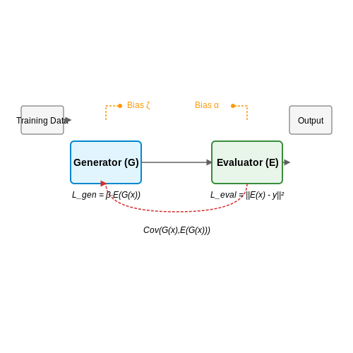
The joint training dynamics of generator-evaluator pairs introduce structural biases. For instance, if the evaluator's loss function dominates the generator's updates, the system may prioritize evaluator-friendly outputs at the expense of diversity. This manifests mathematically as:
where α controls the balance between generation quality and evaluator satisfaction. Improper tuning leads to mode collapse in the generator or evaluator overfitting.
Data-Distribution Bias
Three primary data-related biases affect dual models:
- Representation bias: Underrepresented groups in training data cause the evaluator to develop skewed quality metrics
- Measurement bias: Noisy or incomplete labels propagate through both components
- Selection bias: Non-random sampling during adversarial training creates feedback loops
The bias amplification factor β can be quantified through the covariance between generator outputs and evaluator scores:
Algorithmic Feedback Loops
Dual models exhibit emergent biases through:
- Preference amplification: Small evaluator preferences become dominant features in generated outputs
- Conformity pressure: The generator learns to produce evaluator-high-scoring outputs exclusively
- Reward hacking: The generator discovers shortcuts that artificially inflate evaluator metrics
These effects compound over training iterations according to the recurrence relation:
where γ represents the learning rate and bt the bias at step t.
Mitigation Strategies
Effective bias identification requires monitoring:
- Output distribution KL divergence between generator and training data
- Evaluator score distributions across demographic slices
- Gradient conflict metrics between generator and evaluator
Diagnostic tests should compute the bias susceptibility index:
Values above 1.0 indicate significant bias propagation. Case studies from recommender systems show ζ > 1.5 correlates with measurable real-world discrimination.
5.2 Techniques for Fairness-Aware Training
Fairness Metrics and Constraints
Fairness-aware training requires formalizing fairness as an optimization constraint. Common fairness metrics include:
- Demographic Parity: Requires predictions to be statistically independent of protected attributes (e.g., race, gender). Formally, for a binary classifier h and protected attribute A, demographic parity enforces P(h(x)=1|A=0) = P(h(x)=1|A=1).
- Equalized Odds: Adds the constraint that true positive and false positive rates must be equal across groups: P(h(x)=1|A=0,Y=y) = P(h(x)=1|A=1,Y=y) for y ∈ {0,1}.
- Predictive Rate Parity: Ensures equal positive predictive value across groups: P(Y=1|h(x)=1,A=0) = P(Y=1|h(x)=1,A=1).
Adversarial Debiasing
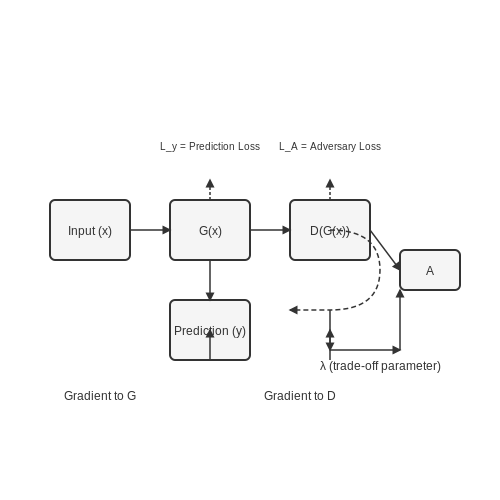
Adversarial training introduces a discriminator network D that attempts to predict the protected attribute from the model's representations. The generator G is trained to both minimize prediction error and maximize the discriminator's error:
where λ controls the trade-off between accuracy and fairness. This approach has been shown effective in NLP and computer vision applications where sensitive attributes may be implicitly encoded in embeddings.
Reweighting and Preprocessing
Sample reweighting adjusts the loss function to account for disparities in group representation or outcomes. For each sample (x,y), compute weights w as:
where Pexp represents the desired distribution and Pobs the observed distribution. This technique is particularly useful when historical bias exists in the training data collection process.
Fairness-Aware Regularization
Regularization terms can directly penalize unfairness metrics in the loss function. For example, a covariance-based regularizer for demographic parity:
where ai is the protected attribute and h̄ is the mean prediction. This approach maintains differentiability while enforcing approximate fairness constraints.
Post-Hoc Calibration
For dual-purpose models, the evaluator component can be designed to output calibrated probabilities that satisfy fairness constraints through:
- Platt Scaling: Learn a sigmoid transformation of evaluator scores to match desired group-wise calibration properties.
- Temperature Scaling: Adjust the softmax temperature separately for different protected groups to equalize confidence distributions.
where Ta are group-specific temperatures learned via constrained optimization.
Implementation Considerations
When implementing fairness-aware training for dual-purpose models:
- The generator and evaluator may require different fairness constraints (e.g., demographic parity for generation, equalized odds for evaluation).
- Batch normalization statistics should be computed separately for different protected groups when using adversarial methods.
- Gradient reversal layers can stabilize training when using adversarial debiasing approaches.
5.3 Transparency and Explainability in Joint Systems
Dual-purpose models combining generation and evaluation require specialized techniques for interpretability, as traditional explainability methods often fail to capture the bidirectional interactions between components. The primary challenge lies in disentangling the generator's influence on the evaluator's decisions and vice versa, particularly when both systems are trained jointly through adversarial or cooperative objectives.
Architectural Decomposition for Interpretability
Joint systems can be analyzed through layer-wise relevance propagation (LRP) adapted for coupled architectures. For a generator G and evaluator E, the relevance R of an input feature xi to the final evaluation score y decomposes as:
where z represents the generator's latent variables. This formulation reveals how input perturbations propagate through both systems. In practice, Monte Carlo sampling estimates these gradients efficiently while handling non-differentiable operations through surrogate gradients.
Counterfactual Analysis in Coupled Systems
Generating meaningful counterfactuals requires modifying the standard approach to account for the evaluator's feedback loop. The optimal counterfactual x' for input x solves:
where λ balances similarity and desired evaluator response. This becomes particularly challenging when E and G share parameters, necessitating techniques like:
- Adversarial masking of shared weights during explanation
- Path-integrated gradients that track contributions through both networks
- Dynamic computational graphs that preserve tensor dependencies
Real-World Implementation Challenges
Industrial applications reveal three key practical considerations:
- Latent space entanglement: Joint training often creates correlated features that resist traditional attribution methods. Spectral clustering of gradient Hessians helps isolate disentangled concepts.
- Feedback delays: In production systems, the evaluator's response may lag the generator's output. Time-dependent Shapley values extend explainability to temporal scenarios.
- Distributional shift: The generator's outputs often lie outside the evaluator's training distribution. Importance weighting of attribution scores compensates for this mismatch.
Quantitative Explainability Metrics
Standard interpretability metrics fail to capture the unique dynamics of joint systems. We propose two specialized measures:
where θG and θE are parameters of generator and evaluator respectively. Values above 1 indicate the generator disproportionately influences decisions. Complementing this, the Explanation Consistency Score (ECS) measures agreement between separate and joint explanations:
Recent work shows optimal transparency occurs when 0.7 ≤ ECS ≤ 0.9, indicating neither complete independence nor total entanglement of explanations.
6. Key Research Papers on Dual-Purpose Models
6.1 Key Research Papers on Dual-Purpose Models
- MOD-026-1: Verification of Models and Data for Generator Excitation ... — Purpose To verify that the generator excitation control system or plant volt/var control function1 model (including the power system stabilizer model and the impedance compensator model) and the model parameters used in dynamic simulations accurately represent the generator excitation control system or plant volt/var control function behavior when assessing Bulk Electric System (BES ...
- PDF Dual Rotor Generator for Increased Efficient Power Generation — 6. DESIGN AND COMPONENTS OF DUAL ROTOR GENERATOR In this Design of dual rotor generator, we have two rotors. 1. Inner rotor 2. Outer rotor Fig. 6.1 : Design of generator coupled with motor 6.1 Inner rotor: It consists of three phase armature winding with 24 slots from which the electric output generated will be taken out through brushes.
- PDF Chapter 6 Mathematical Model of Synchronous Generator and Load - Springer — In Chap. 1, the mathematical model of a power network has been introduced. Mathematical models of HVDC and FACTS are discussed in Chap. 5. Hence, in this chapter the focus is the introduction to mathematical models of generator and load, including the mathematical models of synchronous generator, excitation systems, and governing systems.
- PDF A. Introduction - North American Electric Reliability Corporation — 3. Purpose: To verify that the generator excitation control system or plant volt/var control function. 1. model (including the power system stabilizer model and the impedance compensator model) and the model parameters used in dynamic simulations accurately represent the generator excitation control system or plant volt/var control
- Evaluation of the Time Domain Models of the Wind Turbine Generator and ... — The system description of the controllable grid interface (CGI) and the commercial multi-megawatt sized type 4 wind turbine generator (WTG) installed at the National Renewable Energy Laboratory (NREL) was presented in Chap. 7.Detailed, generic electromagnetic transient (EMT) models of the CGI and the WTG were developed in Chap. 8.The purpose of this chapter is the evaluation of said models.
- Model Classes — deepchem 2.8.1.dev documentation — Namely, that only regression and classification models can be evaluated in this fashion. For generator models, you will need to overwrite this method to perform a custom evaluation. Keyword arguments specified here will be passed to Evaluator.compute_model_performance. Parameters: dataset - Dataset object.
- Modeling of synchronous generators in power system studies - ResearchGate — The gentpf generator model. 3. Comparison of the performance of the four different generator models based on measured on-line response of synchronous machines 3.1.
- PDF Mathematical Models In Electric Power Systems - EOLSS — UNESCO - EOLSS SAMPLE CHAPTERS MATHEMATICAL MODELS - Vol. II - Mathematical Models in Electric Power Systems - Prabha Kundur, Lei Wang ©Encyclopedia of Life Support Systems(EOLSS) PVI= cosφ (15) QVI= sinφ (16) The instantaneous power p(t) thus has two components: 1cos2 sin 2 p q p Pt pQ t ω ω =− = The component pp has an average value of P=VI cos φ, and represents the component of
- PDF Plant Model Generator from Digital Twin for Purpose of Formal Verification — This thesis work builds upon previous work from [1]. The key di erences are related to state machine generation. Their work is about state machine generation for a controller using traces from a real controller, whereas this master thesis takes a look at state machines and formal model generation of plant model using traces from a digital twin
- A review of modelling tools for energy and electricity systems with ... — This paper presents a thorough review of 75 modelling tools currently used for analysing energy and electricity systems. Increased activity within model development in recent years has led to several new models and modelling capabilities, partly motivated by the need to better represent the integration of variable renewables.
6.2 Open-Source Implementations and Toolkits
- EleutherAI/lm-evaluation-harness - GitHub — [2025/03] Added support for steering HF models! [2025/02] Added SGLang support! [2024/09] We are prototyping allowing users of LM Evaluation Harness to create and evaluate on text+image multimodal input, text output tasks, and have just added the hf-multimodal and vllm-vlm model types and mmmu task as a prototype feature. We welcome users to try out this in-progress feature and stress-test it ...
- PDF Coupled Training for Multi-Source Domain Adaptation - CVF Open Access — Figure 2. Decision boundaries of source-only model and MUST. Each colored line corresponds to a different initialization. Blue: positive source samples. Red: negative source samples. Gray: un-labeled target samples. The source-only model is trained only on source samples; it classifies perfectly the source data but ignores the target data.
- Secure Software Development Practices for Generative AI and Dual-Use ... — AI model and system development is still much more of an art than an exact science, requiring developers to interact with model code, training data, and other parameters over multiple iterations. Training datasets may be acquired from unknown, untrusted sources. Model weights and other training parameters can be susceptible to malicious tampering.
- jpmml/jpmml-evaluator: Java Evaluator API for PMML - GitHub — JPMML-Evaluator library JAR files (together with accompanying Java source and Javadocs JAR files) are released via Maven Central Repository.. The current version is 1.7.3 (5 April, 2025).. The main component of JPMML-Evaluator is org.jpmml:pmml-evaluator.However, in most application scenarios, this component is not included directly, but via a data format-specific runtime component(s) org ...
- Understanding GANs: fundamentals, variants, training challenges ... — Generative adversarial networks (GANs), a novel framework for training generative models in an adversarial setup, have attracted significant attention in recent years. The two opposing neural networks of the GANs framework, i.e., a generator and a discriminator, are trained simultaneously in a zero-sum game, where the generator generates images to fool the discriminator that is trained to ...
- MATLAB and Simulink for Artificial Intelligence - MathWorks — Create AI models with a few lines of code or use pretrained models; Use domain-specific tools and low-code apps to build complete and scalable AI workflows; Combine AI techniques with system-level simulation to reduce errors in production; Deploy AI models to high-performance systems, such as edge devices and the cloud
- GitHub - tatsu-lab/alpaca_eval: An automatic evaluator for instruction ... — Leaderboard: a leaderboard of common models on the AlpacaEval evaluation set. Caution: Automatic evaluators (e.g. GPT-4) may be biased towards models that generate longer outputs and/or that were fine-tuned on the model underlying the evaluator (e.g. GPT-4).
- GitHub - deepspeedai/DeepSpeed: DeepSpeed is a deep learning ... — Model Implementations for Inference (MII) is an open-sourced repository for making low-latency and high-throughput inference accessible to all data scientists by alleviating the need to apply complex system optimization techniques themselves. Out-of-box, MII offers support for thousands of widely used DL models, optimized using DeepSpeed-Inference, that can be deployed with a few lines of code ...
- An open-source parallel EMT simulation framework — An open-source Python-based electromagnetic transient (EMT) simulator, named ParaEMT, is developed for simulating large-scale power systems. ParaEMT is easily compatible with the distributed memory paradigm, such as multiple computers on a transmission control protocol (TCP) network and high-performance computing (HPC) protocols.
- Deep Generative Modelling: A Comparative Review of VAEs, GANs ... — Deep generative models are a class of techniques that train deep neural networks to model the distribution of training samples. Research has fragmented into various interconnected approaches, each ...
6.3 Advanced Topics and Emerging Trends
- Li Et Al. - 2023 - Multimodal Foundation Models From Specialists To — This paper presents a comprehensive survey of the taxonomy and evolution of multimodal foundation models that demonstrate vision and vision-language capabilities, focusing on the transition from specialist models to general-purpose assistants. The research landscape encompasses five core topics, categorized into two classes - methods of learning vision backbones for visual understanding and ...
- Segmented thermoelectric generator modelling and optimization using ... — A conventional ANN training involves only one dataset and one step training process as shown in Fig. 3 a. Because the dataset is randomly generated and only contains low-performing TEG designs, the trained ANN (Uni 4000) is only capable of predicting low-performing TEGs. Our novel iterative training process has two steps as shown in Fig. 3 b.
- The Road Ahead: Emerging Trends, Unresolved Issues, and Concluding ... — Throughout the training process, the model endeavors to minimize the negative log-likelihood loss, which quantifies the disparity between the genuine data distribution and the distribution produced by the model. MLE offers a principled and direct method for training generative models by focusing on optimizing the data likelihood . 3.7.2.
- PDF Fictitious GAN: Training GANs with Historical Models - CVF Open Access — The proposed training algorithm is referred to as Fictitious GAN, where the discriminator (resp. generator) is updated based on the the mixed outputs from the sequence of historical trained generators (resp. discriminators). The previ-ously trained models actually carry important information and can be utilized for the updates of the new model.
- Understanding GANs: fundamentals, variants, training challenges ... — Generative adversarial networks (GANs), a novel framework for training generative models in an adversarial setup, have attracted significant attention in recent years. The two opposing neural networks of the GANs framework, i.e., a generator and a discriminator, are trained simultaneously in a zero-sum game, where the generator generates images to fool the discriminator that is trained to ...
- LLM4EDA: Emerging Progress in Large Language Models for Electronic ... — The large circuit model is trained either from scratch or by fine-tuning an existing Language Large Model (LLM) using these data. Once trained, this model can enhance the capabilities of existing EDA tools and facilitate various downstream applications. The ideal workflow, based on the large circuit model, is depicted in Fig. 3. However, it's ...
- Artificial intelligence techniques framework in the design and ... — The studied moth-flame optimisation (MFO) algorithm in Ref. [16] indicated that power converters are the primary enablers of technologies like RES, microgrids, uninterruptible power supply systems, variable speed drives, and EV vehicles and associated charging/storage infrastructure [19, 20].The study in Ref. [21] showed how the ANN methodology balances the output filter size and switch mode ...
- Two-stage surrogate modeling for data-driven design optimization with ... — An emerging approach to inverse analysis revolves around developing machine learning-based surrogate models. A conventional notion of supervised machine learning is to use observations in the form of input-output pairs, known as the training data set, to learn a proxy or surrogate model that mimics the behavior of complex systems for making predictions about unseen or future inputs (Kim and ...
- Generative artificial intelligence: a systematic review and ... — In recent years, the study of artificial intelligence (AI) has undergone a paradigm shift. This has been propelled by the groundbreaking capabilities of generative models both in supervised and unsupervised learning scenarios. Generative AI has shown state-of-the-art performance in solving perplexing real-world conundrums in fields such as image translation, medical diagnostics, textual ...
- PDF Dual Learning - Springer — Preface Deep neural networks have become the dominantparadigm for artificial intelligence (AI)inthepast decade,anddeeplearninghassignificantlyadvancedvariousareasof








