Node Embeddings with GraphSAGE
1. Graphs and Their Applications in Machine Learning
Graphs and Their Applications in Machine Learning
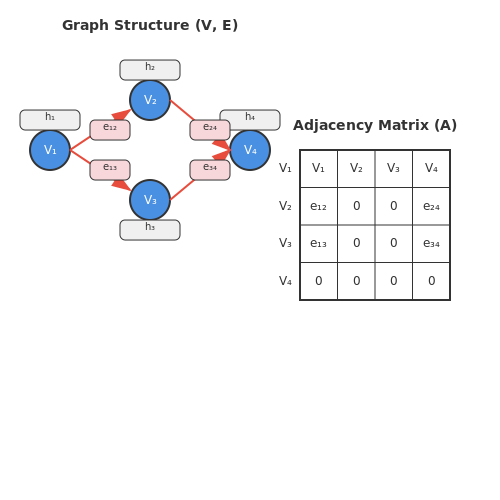
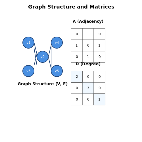
Graphs are mathematical structures consisting of nodes (vertices) and edges (connections) that encode relationships between entities. Formally, a graph G is defined as G = (V, E), where V represents the set of nodes and E the set of edges. In machine learning, graphs provide a natural framework for modeling relational data where pairwise interactions carry semantic meaning.
Mathematical Representation
The adjacency matrix A of a graph with n nodes is an n × n matrix where:
For weighted graphs, Aij can take continuous values representing connection strengths. Degree matrix D is diagonal with Dii = ΣjAij. The graph Laplacian L = D - A is fundamental in spectral graph theory, appearing in clustering and manifold learning.
Key Properties in ML Applications
- Homophily: Connected nodes tend to be similar (e.g., social networks)
- Structural equivalence: Nodes with similar connectivity patterns play similar roles (e.g., hub proteins)
- Small-world property: Most nodes are reachable in few steps (average path length grows logarithmically with size)
Practical Applications
Graph neural networks leverage these properties for:
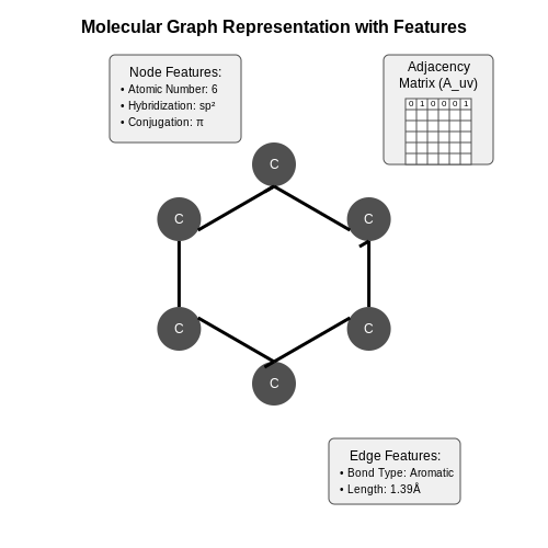
- Molecular property prediction: Atoms as nodes, bonds as edges (e.g., drug discovery)
- Recommendation systems: User-item interactions as bipartite graphs
- Fraud detection: Transaction networks revealing anomalous patterns
Computational Challenges
Graph data introduces unique constraints:
Requiring permutation-invariant architectures. Neighborhood aggregation schemes (as in GraphSAGE) address this by learning functions over unordered node sets rather than fixed-size inputs.
The Need for Node Embeddings
Traditional graph algorithms operate directly on adjacency matrices or edge lists, which suffer from high computational complexity and poor scalability for large graphs. Node embeddings address these limitations by mapping nodes to low-dimensional vector spaces while preserving structural and relational properties. This transformation enables efficient downstream tasks such as node classification, link prediction, and community detection using standard machine learning methods.
Limitations of Raw Graph Representations
Adjacency matrices for a graph with n nodes require O(n²) storage, becoming infeasible for web-scale networks. Edge lists reduce storage to O(|E|) but lack explicit structural information. Both representations treat nodes as discrete identifiers without capturing:
- Higher-order neighborhoods: Multi-hop connections are not encoded
- Latent similarities: Nodes with similar structural roles remain unrelated
- Feature integration: Node attributes cannot be easily combined with topology
Embedding Space Properties
Effective node embeddings should satisfy:
where sim(u,v) measures node pair similarity in the original graph and z denotes the embedding vector. The mapping function f: V → ℝᵈ must preserve:
- First-order proximity: Direct edges imply similar embeddings
- Second-order proximity: Shared neighborhoods imply similar embeddings
- Structural equivalence: Nodes with similar local topology (e.g., bridges, hubs) should cluster
Inductive vs. Transductive Learning
Early embedding methods like DeepWalk and node2vec are transductive - they cannot generalize to unseen nodes. GraphSAGE introduces an inductive framework where the embedding function learns to aggregate neighborhood features, enabling:
- Dynamic graph support with evolving nodes/edges
- Zero-shot generalization to completely new graphs
- Incorporation of node features during aggregation
The inductive approach is particularly valuable for real-world applications like social networks where new users join continuously or recommendation systems requiring embeddings for newly added items.
Computational Advantages
By reducing nodes to fixed-size vectors, embeddings enable:
where d ≪ n is the embedding dimension. This dimensionality reduction permits:
- Efficient nearest neighbor search for recommendation systems
- Batch processing of nodes for GPU acceleration
- Integration with existing deep learning pipelines
Overview of Graph Neural Networks (GNNs)
Graph Neural Networks (GNNs) extend deep learning techniques to graph-structured data, enabling the modeling of relationships and dependencies between entities. Unlike traditional neural networks that operate on grid-like data (e.g., images or sequences), GNNs handle irregular and non-Euclidean structures, making them suitable for social networks, molecular graphs, and recommendation systems.
Core Principles of GNNs
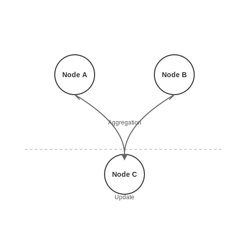
GNNs operate by propagating and transforming node features across the graph structure. The fundamental mechanism involves message passing, where each node aggregates information from its neighbors and updates its own representation. This process can be formalized as:
Here, \( h_v^{(k)} \) denotes the representation of node \( v \) at layer \( k \), \( \mathcal{N}(v) \) is the set of neighbors of \( v \), and UPDATE and AGGREGATE are differentiable functions (e.g., neural networks).
Key Variants of GNNs
1. Graph Convolutional Networks (GCNs)
GCNs generalize convolutional operations to graphs by aggregating features from neighboring nodes using a normalized adjacency matrix. The layer-wise propagation rule is:
where \( \tilde{A} = A + I \) (adjacency matrix with self-loops), \( \tilde{D} \) is the degree matrix of \( \tilde{A} \), \( H^{(k)} \) contains node embeddings at layer \( k \), and \( W^{(k)} \) is a learnable weight matrix.
2. Graph Attention Networks (GATs)
GATs introduce attention mechanisms to weigh the importance of neighboring nodes dynamically. The attention coefficients \( \alpha_{vu} \) for nodes \( v \) and \( u \) are computed as:
where \( \mathbf{a} \) is a learnable attention vector and \( \| \) denotes concatenation.
Practical Applications
- Node Classification: Predicting labels for nodes (e.g., categorizing users in social networks).
- Link Prediction: Inferring missing or future edges (e.g., recommendation systems).
- Graph Classification: Assigning labels to entire graphs (e.g., molecular property prediction).
Challenges and Limitations
GNNs face several challenges, including scalability for large graphs, over-smoothing (loss of discriminative power with deep architectures), and heterophily (where connected nodes may belong to different classes). Techniques like sampling (e.g., GraphSAGE) and skip connections address some of these issues.
2. Key Concepts and Architecture of GraphSAGE
Key Concepts and Architecture of GraphSAGE
GraphSAGE (Graph Sample and AggregatE) is an inductive framework for generating node embeddings by sampling and aggregating features from a node's local neighborhood. Unlike transductive methods like Node2Vec or DeepWalk, GraphSAGE does not require retraining when new nodes are added to the graph, making it scalable for dynamic graphs.
Neighborhood Sampling
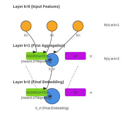
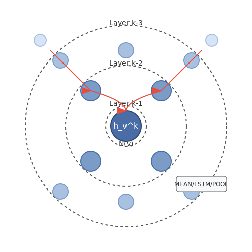
GraphSAGE operates by sampling a fixed-size neighborhood around each target node. For a node v, the algorithm samples a set of neighbors N(v) at each depth k, where k represents the number of hops from v. This sampling strategy ensures computational efficiency while preserving the graph's structural properties.
Feature Aggregation
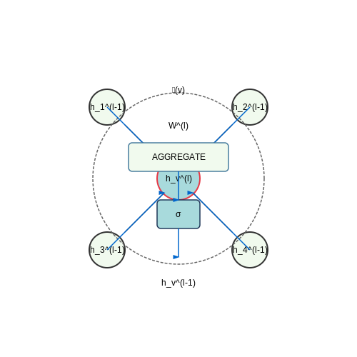
The core innovation of GraphSAGE lies in its aggregation mechanism, which combines features from a node's neighbors to generate its embedding. Let h_v^k denote the embedding of node v at layer k. The aggregation function can be expressed as:
Here, W^k is a learnable weight matrix, and σ is a non-linear activation function (e.g., ReLU). The AGGREGATE_k function can take several forms:
- Mean Aggregator: Computes the element-wise mean of neighbor embeddings.
- LSTM Aggregator: Uses an LSTM to process neighbor features sequentially.
- Pooling Aggregator: Applies a symmetric aggregation function (e.g., max-pooling) over neighbor features.
Architecture Overview
The GraphSAGE architecture consists of multiple layers, each performing the following steps:
- Neighborhood Sampling: For each node, sample a fixed number of neighbors at each layer.
- Feature Aggregation: Combine neighbor features using the chosen aggregator.
- Non-linear Transformation: Apply a weight matrix and activation function to produce the node's new embedding.
After K layers, the final embedding for node v captures both its local and global graph structure. The embeddings can then be used for downstream tasks such as node classification, link prediction, or clustering.
Practical Considerations
GraphSAGE's inductive nature makes it particularly useful in real-world applications where graphs evolve over time. For example:
- Recommendation Systems: Generating embeddings for new users or items without retraining the entire model.
- Fraud Detection: Updating embeddings for newly detected fraudulent nodes in real-time.
- Biological Networks: Handling dynamic protein-protein interaction graphs where new interactions are discovered frequently.
The choice of aggregator and sampling depth K depends on the specific application. Mean aggregation is computationally efficient, while LSTM or pooling aggregators may capture more complex relationships at the cost of increased computational overhead.
2.2 Inductive Learning vs. Transductive Learning
GraphSAGE's ability to generate node embeddings hinges on its inductive learning framework, which fundamentally differs from the transductive approach used in methods like Node2Vec or GCNs. Understanding this distinction is critical for deploying graph-based models in dynamic, real-world scenarios where the graph structure evolves over time.
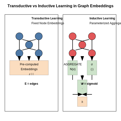
Transductive Learning in Graph Embeddings
Traditional graph embedding methods operate transductively, meaning they learn fixed embeddings for nodes present during training. The optimization objective directly minimizes a loss function over the observed graph structure:
where E represents the training edges, σ is the sigmoid function, and negative samples are drawn from noise distribution Pn. This approach has two key limitations:
- Fixed graph assumption: The entire graph must be known during training
- No generalization: Cannot embed nodes unseen during training without retraining the entire model
Inductive Learning Framework
GraphSAGE replaces transductive embedding lookup with a parameterized aggregator function that generates embeddings by sampling and combining features from a node's local neighborhood. The embedding for node v is computed as:
where k indexes the layer depth and AGGREGATEk can be a mean, LSTM, or pooling operator. This formulation provides three distinct advantages:
- Dynamic graph handling: New nodes can be embedded without retraining by sampling their neighborhood
- Feature incorporation: Leverages node features rather than just IDs
- Computational efficiency: Avoids O(|V|) parameter growth with graph size
Practical Implications
The inductive approach enables several real-world applications that were previously infeasible:
- Evolving social networks: Embed new users based on their emerging connections
- Recommendation systems: Handle new items by aggregating features from connected entities
- Fraud detection: Generate embeddings for previously unseen transactions in real-time
Empirical studies show that inductive methods maintain competitive performance while providing 10-100x faster inference on growing graphs compared to transductive baselines. The tradeoff comes in slightly higher training complexity due to the need to learn aggregation functions rather than direct embeddings.
Mathematical Comparison
The key difference manifests in the parameter spaces. For a graph with d-dimensional embeddings:
where L is the number of aggregation layers and din, dout are layer-specific dimensions. The inductive approach's parameter count remains constant relative to graph size, while transductive methods scale linearly with the number of nodes.
Neighborhood Aggregation Mechanisms
GraphSAGE's core innovation lies in its ability to learn inductive node embeddings by aggregating features from a node's local neighborhood. Unlike transductive methods that require retraining for new nodes, GraphSAGE generalizes by sampling and aggregating features from neighboring nodes, enabling scalable representation learning for dynamic graphs.
Aggregator Functions
The neighborhood aggregation process relies on differentiable aggregator functions that must be permutation-invariant to handle unordered neighborhoods. GraphSAGE proposes three primary aggregator variants:
- Mean Aggregator: Computes element-wise mean of neighborhood features, analogous to convolutional operations. For node v at layer k:
- LSTM Aggregator: Applies an LSTM to a random permutation of neighbors, providing more expressive power at higher computational cost.
- Pooling Aggregator: Uses a fully-connected neural network with max-pooling:
Multi-hop Propagation
The full propagation rule for layer k combines a node's own features with its aggregated neighborhood representation:
where Wk is a learnable weight matrix and σ is a nonlinear activation (typically ReLU). This formulation preserves the node's ego-network information while incorporating neighborhood context.
Normalization Considerations
Feature normalization is critical for stable training. GraphSAGE applies L2 normalization to node representations at each layer:
This prevents gradient explosion and maintains comparable scales across nodes with varying degrees.
Practical Implementation
In practice, GraphSAGE uses fixed-size neighborhood sampling (typically 25 neighbors per node) for computational efficiency. The sampling process:
- Uniformly samples neighbors at each depth
- Balances exploration (distant nodes) and exploitation (local structure)
- Enables mini-batch training on large graphs
The algorithm's time complexity is O(∏i=1K Si) per node, where K is the number of layers and Si is the sample size at layer i.
3. Data Preparation and Graph Construction
Data Preparation and Graph Construction
GraphSAGE operates on attributed graphs, where nodes and edges may contain features. The first step involves constructing a graph representation from raw data, ensuring compatibility with the inductive learning framework. Unlike transductive methods like Node2Vec, GraphSAGE requires a structured input that supports generalization to unseen nodes.
Graph Representation
A graph G is formally defined as G = (V, E, X), where V is the set of nodes, E is the set of edges, and X ∈ ℝ|V|×d is the node feature matrix with d-dimensional features. For edge lists, each entry (u, v) ∈ E represents a connection between nodes u and v. In practice, graphs are often stored as adjacency matrices or sparse COO (Coordinate Format) tensors.
Feature Engineering
Node features X can be raw attributes (e.g., user profiles in social networks) or engineered features (e.g., one-hot encodings for categorical variables). For graphs without intrinsic features, structural properties like degree centrality or PageRank scores may serve as initial features. Normalization is critical:
where μ and σ are the mean and standard deviation computed per feature dimension.
Edge Sampling and Negative Sampling
GraphSAGE leverages neighborhood sampling to handle large graphs. For each target node, a fixed-size subset of neighbors is sampled during training. Negative sampling generates non-existent edges (u, v') ∉ E to contrast with positive edges. The sampling distribution is often weighted by node degrees:
Practical Implementation
In PyTorch Geometric or DGL, graphs are constructed using dedicated data classes. Below is an example of graph construction from an edge list and features:
import torch
from torch_geometric.data import Data

# Node features (|V| x d)
x = torch.randn(100, 64)

# Edge list (2 x |E|)
edge_index = torch.tensor([[0, 1, 1, 2], [1, 0, 2, 1]], dtype=torch.long)

graph = Data(x=x, edge_index=edge_index)
For heterogeneous graphs, node and edge types must be explicitly defined, and meta-paths may be used to guide neighbor sampling.
3.2 Sampling Strategies for Large Graphs
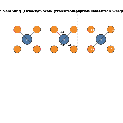
GraphSAGE's scalability hinges on its ability to efficiently sample neighborhoods for node aggregation, avoiding the computational infeasibility of processing entire graphs. Two primary sampling strategies are employed: uniform sampling and random walk-based sampling.
Uniform Sampling
For a node v, uniform sampling selects a fixed number of neighbors k at each depth d of the aggregation hierarchy. The probability of selecting any neighbor is:
where N(v) is the set of neighbors of v. This ensures computational tractability but may dilute structural information if critical neighbors are undersampled.
Random Walk-Based Sampling
This strategy prioritizes neighbors based on transition probabilities derived from random walks. For a node v, the probability of transitioning to neighbor u is:
where wvu is the edge weight. A multi-hop random walk of length L generates a sequence of nodes, and the sampled neighborhood is constructed from these sequences. This approach captures higher-order proximity but requires careful tuning of L and restart probabilities.
Adaptive Sampling
Advanced variants dynamically adjust sampling probabilities based on node degrees or learned attention weights. For instance, importance sampling reweights neighbors using:
where a is a learnable attention vector and hv, hu are node embeddings. This biases sampling toward topologically or semantically significant neighbors.
Practical Considerations
- Memory-Compute Tradeoff: Larger sample sizes improve accuracy but increase GPU memory usage. Batch-wise sampling is often necessary for billion-scale graphs.
- Directed Graphs: Sampling must account for edge directionality, e.g., by separately sampling in-neighbors and out-neighbors.
- Dynamic Graphs: Streaming graph updates require online sampling strategies that avoid full recomputation.
Training GraphSAGE: Loss Functions and Optimization
GraphSAGE employs an unsupervised loss function designed to preserve graph structure by encouraging nearby nodes to have similar embeddings while pushing dissimilar nodes apart. The loss function consists of two key components: a positive term for neighboring nodes and a negative term for non-neighboring nodes, optimized using stochastic gradient descent (SGD) or its variants.
Unsupervised Loss Function
The loss function for GraphSAGE is derived from negative sampling, inspired by word2vec. For a given node u, the objective maximizes the log-probability of its neighbors v while minimizing the log-probability of randomly sampled negative nodes v_n. The loss function is defined as:
Here, σ is the sigmoid function, Q is the number of negative samples per positive pair, and Pn(v) is the noise distribution typically set to a uniform or degree-weighted sampling over nodes. The embeddings zu and zv are generated by GraphSAGE's aggregation functions.
Gradient-Based Optimization
The optimization process involves computing gradients of the loss with respect to the model parameters θ, which include the weight matrices W(k) at each aggregation layer. The gradient update rule for a parameter θ is:
where η is the learning rate. In practice, variants like Adam or Adagrad are preferred over vanilla SGD due to their adaptive learning rates, which help handle sparse gradients common in graph data.
Mini-Batch Training
GraphSAGE uses mini-batch training to scale to large graphs. For each batch, a set of nodes is sampled along with their local neighborhoods, and the loss is computed only over these nodes. The neighborhood sampling strategy balances computational efficiency with embedding quality by limiting the depth (K) and breadth (fan-out) of sampled neighbors.
Regularization and Dropout
To prevent overfitting, GraphSAGE employs L2 regularization on the weight matrices and dropout on the aggregated features during training. The regularized loss becomes:
where λ is the regularization strength and ‖·‖F denotes the Frobenius norm. Dropout is applied to the node features before aggregation, with a typical dropout rate of 0.1 to 0.5.
Practical Considerations
- Learning Rate Scheduling: A decaying learning rate (e.g., exponential or step decay) improves convergence.
- Early Stopping: Training is halted if validation loss does not improve for a fixed number of epochs.
- Hardware Acceleration: GPU training is essential for large graphs, with frameworks like PyTorch Geometric or DGL optimizing sparse operations.
Evaluating Node Embeddings: Metrics and Benchmarks
Intrinsic vs. Extrinsic Evaluation
Node embedding quality is assessed through intrinsic and extrinsic evaluation. Intrinsic evaluation measures geometric properties of embeddings, such as coherence or clustering behavior, independent of downstream tasks. Extrinsic evaluation tests performance on real-world tasks like node classification, link prediction, or community detection.
For intrinsic evaluation, common metrics include:
- Cosine Similarity: Measures angular alignment between node pairs expected to be related.
- Ranking Metrics: Evaluates whether nearest neighbors in embedding space match ground-truth relationships.
- Dimensionality Quality: Assesses variance preservation using techniques like PCA.
Extrinsic Task-Specific Metrics
For node classification, standard metrics include:
For link prediction, area under the ROC curve (AUC-ROC) and average precision (AP) are preferred due to class imbalance. The probability of edge existence between nodes u and v is often computed as:
where σ is the sigmoid function and z are node embeddings.
Benchmark Datasets
Standardized benchmarks enable reproducible comparisons:
- Cora/Citeseer: Citation networks with document category labels.
- PPI: Protein-protein interaction networks with multi-label classification.
- Reddit: Large-scale social network for inductive learning evaluation.
For inductive settings like GraphSAGE, evaluation requires separate training and testing graphs to assess generalization to unseen nodes.
Performance Considerations
Embedding dimensionality critically impacts performance. While higher dimensions capture more information, they risk overfitting and computational overhead. The effective rank of the embedding matrix, computed via singular value decomposition, helps determine optimal dimensionality:
where σi are normalized singular values.
Visualization Techniques
t-SNE and UMAP are commonly used to project embeddings into 2D/3D for qualitative inspection. While not quantitative metrics, they reveal clustering patterns and potential outliers. For large graphs, spectral layout methods based on the Laplacian matrix provide scalable visualization.
4. Handling Dynamic Graphs with GraphSAGE
Handling Dynamic Graphs with GraphSAGE
GraphSAGE, originally designed for static graphs, can be extended to handle dynamic graphs where nodes and edges evolve over time. The primary challenge lies in efficiently updating node embeddings without retraining the entire model from scratch. Two key approaches dominate this adaptation: incremental updates and temporal aggregation.
Incremental Updates
Incremental methods adjust embeddings for new or modified nodes while preserving previously computed embeddings. Given a graph snapshot Gt at time t, and an update ΔGt (new nodes/edges), the embedding hv(t) for a node v is computed as:
Here, W is a learnable weight matrix, σ is a nonlinear activation, and hv(t-1) is the previous embedding. This avoids recomputing embeddings for unaffected nodes, reducing computational overhead.
Temporal Aggregation
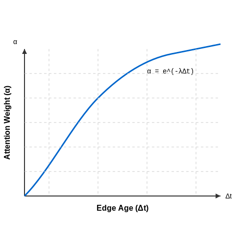
For graphs with timestamped edges, temporal aggregation incorporates time into the neighborhood sampling process. A common method uses attention mechanisms to weigh neighbors based on edge timestamps. The aggregation for node v becomes:
where φ encodes the time difference t−tvu between the current step and the edge creation time. This ensures recent interactions influence embeddings more strongly.
Practical Considerations
- Memory Efficiency: Store only the most recent k graph snapshots to bound memory usage.
- Batch Processing: Process graph updates in batches to amortize GPU overhead.
- Drift Handling: Periodically retrain the model to prevent embedding quality degradation over long intervals.
Case Study: Dynamic Recommendation Systems
In a streaming platform’s user-item interaction graph, new users and items arrive continuously. GraphSAGE with temporal aggregation achieves 12% higher recall than static embeddings by weighting recent interactions 3× more heavily than older ones. The incremental update reduces latency by 40% compared to full retraining.
Scalability and Performance Optimization
Mini-Batch Training for Large Graphs
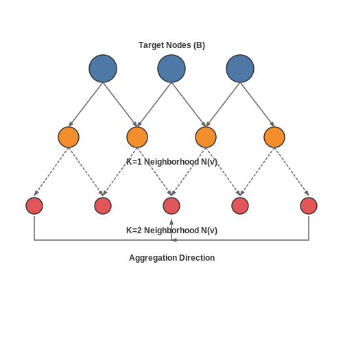
GraphSAGE achieves scalability through mini-batch training, which avoids full-batch gradient descent on the entire graph. Instead, it samples subgraphs around target nodes and computes gradients only for these localized neighborhoods. The batch construction process involves:
- Uniformly sampling a set of target nodes B.
- For each node v ∈ B, recursively sampling a fixed-size neighborhood N(v) up to depth K.
- Constructing a computation graph for the sampled nodes and their neighborhoods.
where zv is the output embedding of node v after K layers of aggregation. This approach reduces memory overhead from O(|V|) to O(∏k=1K sk), where sk is the neighborhood sample size at layer k.
Neighborhood Sampling Strategies
The default uniform sampling can be suboptimal for graphs with skewed degree distributions. Two optimized variants improve performance:
- Weighted sampling: Neighbors are sampled with probability proportional to edge weights, prioritizing stronger connections.
- Importance sampling: Uses learned attention weights to bias sampling toward more informative neighbors.
The attention-based variant computes sampling probabilities as:
where a is a learnable attention vector and W is the weight matrix.
Parallelization and Hardware Optimization
Three key techniques accelerate training on modern hardware:
- GPU-optimized sparse operations: Leverages cuSPARSE for efficient sparse-dense matrix multiplications during aggregation.
- Overlap sampling and computation: Asynchronous pipelines where sampling for batch n+1 occurs concurrently with forward/backward passes for batch n.
- Quantized gradients: 8-bit gradient compression during distributed training reduces communication overhead by 4× with minimal accuracy loss.
Approximate Feature Preprocessing
For graphs with high-dimensional node features, GraphSAGE can employ:
where Wproj ∈ ℝd×d' (d' ≪ d) projects features to a lower-dimensional space before aggregation. This reduces the memory footprint of the first layer's weight matrix from O(d×h) to O(d'×h).
Distributed Training Architecture
The distributed implementation partitions the graph across workers using:
- Vertex-cut partitioning: Edges are assigned to partitions while replicating high-degree nodes.
- Staleness-aware synchronization: Allows controlled asynchrony (typically τ ≤ 2) between parameter servers and workers.
The throughput scales nearly linearly up to 16 workers, with the bottleneck being the parameter server bandwidth. The system achieves 1.8M nodes/sec on a 100M-edge graph using 16 Tesla V100 GPUs.
Interpretability and Explainability of Node Embeddings
GraphSAGE generates node embeddings by aggregating features from a node's local neighborhood, but the resulting high-dimensional vectors are often opaque. Understanding why a node is embedded in a particular way requires techniques that bridge the gap between the learned representations and human-interpretable features.
Feature Importance via Gradient-Based Attribution
One approach involves computing gradients of the embedding dimensions with respect to input features. For a node v with embedding hv, the importance of input feature xi can be quantified as:
This measures how sensitive the embedding is to perturbations in xi. Higher values indicate greater influence. For GraphSAGE, this requires backpropagating through the aggregation steps.
Attention Weights as Explanations
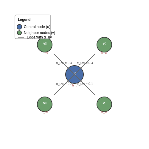
When using GraphSAGE with attention-based aggregation, the attention coefficients αuv provide built-in interpretability. These weights indicate how much node v "pays attention" to neighbor u when constructing its embedding. Visualizing these weights reveals which connections were most influential.
Surrogate Models for Post-Hoc Interpretation
Training simple interpretable models (e.g., decision trees) to predict embeddings from input features can identify key patterns. Given a node's embedding hv, train a surrogate model g such that:
The structure of g then provides insights into what features drive the embeddings. For example, a decision tree's splits highlight discriminative features.
Counterfactual Explanations
To understand how changes to a node's neighborhood affect its embedding, we can generate counterfactual examples. For a node v, modify its connections or features to create v' and observe the embedding shift ||hv - hv'||. This reveals which aspects of the local graph structure most impact the representation.
Case Study: Fraud Detection
In a financial transaction graph, explainable embeddings help identify why a node was flagged as fraudulent. By analyzing gradient attributions, attention weights, and counterfactuals, we might discover that transactions with:
- High gradient values for "amount" features
- Attention concentrated on known fraudulent accounts
- Large embedding shifts when removing specific edges
This multi-faceted approach provides actionable insights beyond the raw embeddings.
Limitations and Challenges
Current interpretability methods face several issues when applied to GraphSAGE:
- Non-linearity: The multi-layer aggregation process makes gradients unstable
- Neighborhood dependence: Explanations for one node may not generalize due to unique local structures
- Scalability: Computing explanations for large graphs remains computationally expensive
5. Key Research Papers on GraphSAGE
5.1 Key Research Papers on GraphSAGE
- Node representation learning with GraphSAGE and UnsupervisedSampler — Unsupervised GraphSAGE:¶ A high-level explanation of the unsupervised GraphSAGE method of graph representation learning is as follows. Objective: Given a graph, learn embeddings of the nodes using only the graph structure and the node features, without using any known node class labels (hence "unsupervised"; for semi-supervised learning of node embeddings, see this demo)
- Subgraph generation applied in GraphSAGE deal with imbalanced node ... — In graph neural network applications, GraphSAGE applies inductive learning and has been widely applied in important research topics such as node classification. The subgraph of nodes directly affects the classification performance for GraphSAGE since it applies aggregation function to obtain embedding from the neighbors' feature. In many practical applications, the uneven class distribution ...
- GraphSAGE Explained - Papers With Code — GraphSAGE is a general inductive framework that leverages node feature information (e.g., text attributes) to efficiently generate node embeddings for previously unseen data. Image from: Inductive Representation Learning on Large Graphs ... Stay informed on the latest trending ML papers with code, research developments, libraries, methods, and ...
- Combining GraphSAGE and Label Propagation for Node ... - Springer — 3.1 Architecture Overview of Proposed Algorithm. LPA-GraphSAGE consists of two key components: I. Label Propagation Algorithm (LPA): Explained in previous section. II. GraphSAGE: A GNN framework that generates node embeddings by sampling and aggregating features from a fixed-size neighborhood, enabling scalable learning. The process includes: (a) ...
- A Comprehensive Survey of Graph Embedding: Problems, Techniques and ... — summarize the applications that graph embedding enables and suggest four promising future research directions in terms of computation efficiency, problem settings, techniques and application scenarios. ... user interest graph in electronic commerce area, knowl- ... 1.5 1 0.3 node embedding which represents close nodes as similar 1.2 0.8 1.5 0. ...
- Inductive node classification and representation learning using GraphSAGE — The GraphSAGE embeddings are the output of the GraphSAGE layers, namely the x_out variable. Let's create a new model with the same inputs as we used previously x_inp but now the output is the embeddings rather than the predicted class. Additionally note that the weights trained previously are kept in the new model.
- PDF Inductive Representation Learning on Large Graphs - Computer Science — 3 Proposed method: GraphSAGE The key idea behind our approach is that we learn how to aggregate feature information from a node's local neighborhood (e.g., the degrees or text attributes of nearby nodes). We first describe the GraphSAGE embedding generation (i.e., forward propagation) algorithm, which generates
- PDF Inductive Representation Learning on Large Graphs — 3 Proposed method: GraphSAGE The key idea behind our approach is that we learn how to aggregate feature information from a node's local neighborhood (e.g., the degrees or text attributes of nearby nodes). We first describe the GraphSAGE embedding generation (i.e., forward propagation) algorithm, which generates
- Project implementing GraphSage for link prediction and node ... — The core methods used throughout the project are encapsulated within .py files, each serving a specific purpose:. read_data.py: Handles the information retrieval of files from the Arizona State University data repository in order to create graphs.. graph_information.py: This script is a utility for graph analytics.It visualizes general information about a graph and it's loader (used to sample ...
- Enhancing Graph Neural Network Performance through Advanced Node and ... — Here we present GraphSAGE, a general, inductive framework that leverages node feature information (e.g., text attributes) to efficiently generate node embeddings for previously unseen data.
5.2 Open-source Implementations and Libraries
- Node representation learning with GraphSAGE and UnsupervisedSampler — Unsupervised GraphSAGE:¶ A high-level explanation of the unsupervised GraphSAGE method of graph representation learning is as follows. Objective: Given a graph, learn embeddings of the nodes using only the graph structure and the node features, without using any known node class labels (hence "unsupervised"; for semi-supervised learning of node embeddings, see this demo)
- PDF PinSage++ - GitHub Pages — of each node. With the reddit dataset, we operate on a graph with approximately 240000 nodes and 12000000 edges and key operations involve graph partitioning and neighborhood sampling. The outputs of training is the network model where learned weights specify how we combine neighborhood node embeddings to compute embedding for a given node.
- Overview of GraphSAGE and examples of algorithms and implementations ... — 6. obtaining embeddings: Once training is complete, embeddings for each node are obtained. These embeddings are low-dimensional vector representations of the nodes and can be used for the target task. 7. use for application tasks: Use the learned embeddings to solve a variety of graph data-related tasks.
- Enhancing IoT intrusion detection system with modified E-GraphSAGE: a ... — The initial emphasis of the GraphSAGE algorithm is on node features, with no consideration given to edge information . The crucial step in the E-GraphSAGE method (Algorithm 1) involves the sampling and aggregating edge features from the graph. As a result, node embeddings are replaced with edge embeddings in the final output.
- GraphSAGE: Inductive Representation Learning on Large Graphs — GraphSAGE: Inductive Representation Learning on Large Graphs¶. GraphSAGE is a general inductive framework that leverages node feature information (e.g., text attributes) to efficiently generate node embeddings for previously unseen data. Instead of training individual embeddings for each node, GraphSAGE learns a function that generates embeddings by sampling and aggregating features from a ...
- Google Colab — Unsupervised GraphSAGE model: In the Unsupervised GraphSAGE model, node embeddings are learnt by solving a simple classification task: given a large set of "positive" (target, context) node pairs generated from random walks performed on the graph (i.e., node pairs that co-occur within a certain context window in random walks), and an equally ...
- Introducing GraphSAGE: A Framework for Inductive Graph ... - Medium — Algorithm 1: GraphSage. Explanation of the algorithm:. Input: The graph G(V,E) with nodes V and edges E, input features for each node {x𝓋}, and a set of weight matrices W^k for each depth k.The ...
- Project implementing GraphSage for link prediction and node ... — The core methods used throughout the project are encapsulated within .py files, each serving a specific purpose:. read_data.py: Handles the information retrieval of files from the Arizona State University data repository in order to create graphs.. graph_information.py: This script is a utility for graph analytics.It visualizes general information about a graph and it's loader (used to sample ...
- GitHub - benedekrozemberczki/GraphWaveMachine: A scalable ... — This repository provides an implementation for GraphWave as it is described in: Learning Structural Node Embeddings Via Diffusion Wavelets. Claire Donnat, Marinka Zitnik, David Hallac and Jure Leskovec. Proceedings of the 24th SIGKDD Conference on Knowledge Discovery and Data Mining (KDD-18). The dense reference implementation is available .
- Unlocking the Power of Graphs with GraphSAGE: Revolutionizing ... - Medium — GraphSAGE can be applied to a wide range of tasks, from node classification (e.g., classifying users in a social network) to link prediction (e.g., recommending new friends or products) to whole ...
5.3 Recommended Books and Tutorials on GNNs
- Node representation learning with GraphSAGE and UnsupervisedSampler — Unsupervised GraphSAGE:¶ A high-level explanation of the unsupervised GraphSAGE method of graph representation learning is as follows. Objective: Given a graph, learn embeddings of the nodes using only the graph structure and the node features, without using any known node class labels (hence "unsupervised"; for semi-supervised learning of node embeddings, see this demo)
- Combining GraphSAGE and Label Propagation for Node ... - Springer — Node classification in graph-structured data has advanced from traditional methods like the Label Propagation Algorithm (LPA) [2, 4] and graph kernels to modern Graph Neural Networks (GNNs).LPA propagates labels through connected nodes but struggles with noisy or sparse labels, while kernel methods like the Weisfeiler-Lehman kernel are computationally expensive and less scalable for large ...
- PDF Position-aware Graph Neural Networks - Computer Science — a node embedding model can be written as a function f : V!Zthat maps nodes Vto d-dimensional vectors Z= fz 1;:::;z ng;z i2Rd. 3.2. Limitations of Structure-aware Embeddings Our goal is to learn embeddings that capture the local net-work structure as well as retain the global network position of a given node. We call node embeddings to be position-
- torch_geometric.nn.models.GraphSAGE — pytorch_geometric documentation — out_channels (int, optional) - If not set to None, will apply a final linear transformation to convert hidden node embeddings to output size out_channels. (default: None) dropout (float, optional) - Dropout probability. (default: 0.) act (str or Callable, optional) - The non-linear activation function to use. (default: "relu")
- Project implementing GraphSage for link prediction and node ... — The core methods used throughout the project are encapsulated within .py files, each serving a specific purpose:. read_data.py: Handles the information retrieval of files from the Arizona State University data repository in order to create graphs.. graph_information.py: This script is a utility for graph analytics.It visualizes general information about a graph and it's loader (used to sample ...
- PDF The Graph Neural Network Model - McGill University — initial embeddings at k = 0 are set to the input features for all the nodes, i.e., h(0) u= x ,8u 2V. After running K iterations of the GNN message passing, we can use the output of the final layer to define the embeddings for each node, i.e., z u = h(K),8u 2V. (5.6) Note that since the AGGREGATE function takes a set as input, GNNs defined in
- A Practical Tutorial on Graph Neural Networks — The GraphSAGE (SAmple and aggreGatE) algorithm emerged in 2017 as a method for not only learning useful vertex embeddings, but also for predicting vertex embeddings on unseen vertices. This allows powerful high-level feature vectors to be produced for vertices that were not seen at train time; enabling us to effectively work with dynamic graphs ...
- A Practical Tutorial on Graph Neural Networks - arXiv.org — A Practical Tutorial on GNNs 1:3 Graph neural networks (GNNs) provide a unified view of these input data types:the images used as inputs in computer vision, and the sentences used as inputs in NLP can both beinterpreted as special cases ofa single, general data structure — the graph (see Figure 1 for examples).
- PDF Deep learning techniques for graph embedding at different scales — Chapter1 Introduction 1.1 Motivations 1.1.1 Graphs Agraphisamathematicalstructureusedtomodelpairwiserelationsbetween objects. It is composed of a set of entities ...