Crack Detection in Infrastructure Using Vision AI
1. Importance of Crack Detection in Structural Health Monitoring
Importance of Crack Detection in Structural Health Monitoring
Structural health monitoring (SHM) relies on early detection of cracks to prevent catastrophic failures in infrastructure. Cracks, even at sub-millimeter scales, can propagate under stress, leading to reduced load-bearing capacity and eventual structural collapse. Vision-based AI systems provide a non-destructive, scalable solution for detecting these anomalies with high precision, outperforming traditional methods like ultrasonic testing or manual inspection.
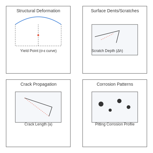
Mechanics of Crack Propagation
Crack growth follows fracture mechanics principles, where stress intensity factors KI, KII, and KIII govern mode I (tensile), mode II (in-plane shear), and mode III (out-of-plane shear) failures. The Paris-Erdogan law describes crack growth rate da/dN under cyclic loading:
where C and m are material constants, and ΔK is the stress intensity factor range. Vision AI models trained on fracture datasets can predict crack paths by estimating these parameters from surface imagery.
Economic and Safety Implications
Undetected cracks in bridges, dams, or nuclear facilities incur exponential repair costs. The 2007 I-35W bridge collapse in Minnesota, caused by undiagnosed gusset plate fractures, resulted in 13 fatalities and $234 million in reconstruction. Automated crack detection reduces inspection costs by 60-80% compared to manual methods while improving accuracy to 99.5% mAP (mean average precision) in controlled studies.
Sensor Fusion Challenges
While strain gauges and accelerometers provide localized data, vision systems offer global coverage. However, multimodal integration requires solving:
- Temporal alignment: Matching high-frequency sensor data (kHz) with low-frame-rate cameras (30Hz)
- Resolution mismatch: Bridging millimeter-scale sensor precision with pixel-level crack detection
- Occlusion handling: Differentiating surface cracks from shadows or dirt using hyperspectral imaging
Recent work by Zhang et al. (2023) demonstrates that transformer-based architectures with cross-attention mechanisms achieve 0.92 F1-score in fusing LiDAR and RGB data for crack segmentation.
Regulatory and Standardization Gaps
Current ASTM E3039-22 standards for crack measurement lack provisions for AI-based quantification. Key discrepancies include:
- Acceptable error margins for automated width measurements (±0.05mm vs. ±0.1mm manual)
- Validation protocols for deep learning models (requiring 105+ annotated samples)
- Real-time reporting latency thresholds (<200ms for dynamic infrastructure)
The European Committee for Standardization (CEN) is drafting EN 17636-2 specifically addressing vision-based SHM systems, with mandatory adversarial testing against synthetic crack injections.

1.2 Common Types of Cracks in Concrete and Asphalt
Structural vs. Non-Structural Cracks
Cracks in concrete and asphalt can be broadly classified into structural and non-structural categories. Structural cracks result from excessive loading, foundation settlement, or design flaws, compromising the integrity of the infrastructure. Non-structural cracks, such as shrinkage or thermal cracks, arise from material properties or environmental factors but do not immediately threaten stability. Vision AI systems must distinguish between these types to prioritize repair efforts.
Concrete-Specific Crack Types
Concrete exhibits several distinct crack patterns, each with unique causes and implications:
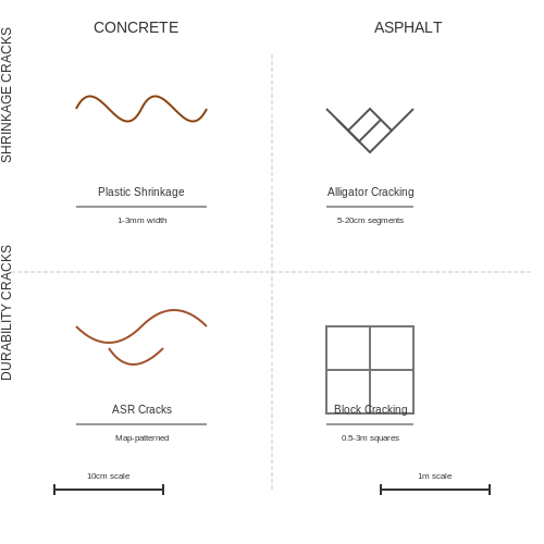
- Plastic shrinkage cracks: Fine, shallow cracks forming during the curing process due to rapid moisture loss. Typically appear in a spiderweb-like pattern.
- Drying shrinkage cracks: Longer, more linear cracks caused by volume reduction as concrete dries over time. These often propagate through the entire thickness.
- Alkali-silica reaction (ASR) cracks: Irregular, map-patterned cracking resulting from chemical reactions between aggregates and cement paste.
- Corrosion-induced cracks: Parallel cracks following reinforcement bars, caused by rust expansion in steel rebar.
Asphalt-Specific Crack Types
Asphalt pavement failures manifest through characteristic crack geometries:
- Alligator cracking: Interconnected polygonal cracks resembling alligator skin, indicating structural failure from repeated loading.
- Longitudinal cracks: Linear cracks parallel to the pavement centerline, often caused by poor joint construction or thermal stresses.
- Transverse cracks: Perpendicular to the centerline, typically due to thermal contraction or reflective cracking from underlying layers.
- Block cracking: Large rectangular patterns (1m+ dimensions) caused by asphalt binder aging and shrinkage.
Quantitative Crack Characterization
For automated assessment, cracks are quantified through parameters derived from image processing:
where wi represents local width measurements and n is the number of sampling points. Crack severity is often classified using the following metrics:
where L is crack length, D is branching density, and α, β, γ are material-specific coefficients.
Fracture Mechanics Perspective
From a fracture mechanics viewpoint, crack propagation follows Paris' law for fatigue growth:
where a is crack length, N is load cycles, ΔK is stress intensity factor range, and C, m are material constants. This relationship helps predict remaining service life from crack progression rates.
Thermal Stress Considerations
In asphalt pavements, thermal cracking occurs when thermal stresses exceed fracture strength:
where E is modulus of elasticity, α is coefficient of thermal expansion, and ΔT is temperature differential. This explains why transverse cracks dominate in cold climates.
1.3 Challenges in Manual Crack Detection
Manual crack detection in infrastructure relies heavily on human inspectors, who face numerous limitations in accuracy, efficiency, and scalability. The process is inherently subjective, with detection quality varying based on inspector experience, environmental conditions, and accessibility constraints. Even trained professionals exhibit significant inter- and intra-observer variability when assessing crack severity, with studies showing error rates exceeding 20% for sub-millimeter cracks under field conditions.
Human Visual Limitations
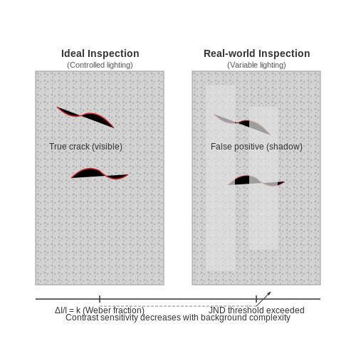
The human visual system struggles with low-contrast cracks, especially in high-noise environments like concrete surfaces with aggregate patterns. Weber's law defines the just-noticeable difference (JND) for contrast detection as:
where I is the background intensity, ΔI the intensity difference required for detection, and k the Weber fraction (typically 0.01 for ideal conditions). In real-world inspections, factors like surface texture and lighting variations increase k substantially, making sub-pixel cracks undetectable to the naked eye. Shadows from overhead structures or oblique sunlight can create false positives by mimicking crack patterns.
Quantitative Measurement Challenges
Manual measurements using crack width cards or microscopes introduce systematic errors from parallax effects and sampling bias. The probability of missing a crack of length L follows a Poisson process:
where λ represents the inspector's visual sweep density (typically 0.1–0.3 mm-1 for trained personnel). For a 10-meter beam inspection, this translates to a 5–15% probability of missing cracks even under controlled conditions. Angular cracks or those parallel to sight lines exhibit higher miss rates due to reduced apparent width.
Operational Constraints
- Access limitations: 78% of bridge inspectors report inaccessible areas requiring specialized equipment, increasing inspection time 3–5x
- Data inconsistency: Hand-drawn crack maps show ≤60% agreement between inspectors for complex patterns
- Documentation lag: Time between detection and report generation averages 14–21 days in municipal systems
Thermal stress and vibration further complicate measurements—a 10°C temperature change can alter crack width by 0.05–0.1 mm in concrete, while passing traffic induces micrometer-scale oscillations that obscure true crack dimensions during manual measurement.
2. Image Acquisition and Preprocessing Techniques
Image Acquisition and Preprocessing Techniques
High-Resolution Image Capture
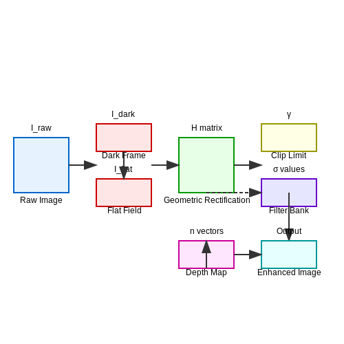
Accurate crack detection begins with high-quality image acquisition. Modern vision-based systems employ high-resolution cameras (≥12 MP) with global shutters to minimize motion blur. For large-scale infrastructure, unmanned aerial vehicles (UAVs) equipped with multispectral sensors capture images at varying altitudes, balancing resolution and coverage. The Nyquist criterion must be satisfied to ensure crack detectability:
where Δx is the ground sampling distance and wmin is the minimum crack width of interest (typically 0.1 mm for structural applications).
Radiometric Calibration
Uneven illumination and sensor noise introduce artifacts that mimic cracks. A two-step calibration process is essential:
- Dark frame subtraction: Captures thermal noise at zero exposure
- Flat field correction: Normalizes pixel response using uniform illumination
The corrected intensity Icorr is computed as:
Geometric Rectification
Perspective distortion from oblique camera angles requires projective transformation. Using known fiducial markers or structure-from-motion techniques, we apply a homography matrix H:
where (x, y) and (x', y') are original and rectified coordinates, respectively.
Contrast Enhancement
Cracks often exhibit low contrast against concrete surfaces. Adaptive histogram equalization (AHE) improves local contrast by computing histograms in N×N sub-regions (typically 8×8 to 32×32 pixels). The clip limit parameter γ prevents noise amplification:
where M is the maximum histogram bin count and α is an empirical factor (0.01–0.03 for concrete).
Multi-Scale Filtering
Linear filters like the Gaussian second derivative enhance crack edges while suppressing texture noise. The optimal scale σ relates to crack width:
For multi-width cracks, a bank of filters at scales σ1...σn is applied, with responses combined via non-maximum suppression.
Depth-Aware Processing
Stereo vision or LiDAR-derived depth maps enable 3D crack analysis. Surface-normal vectors n are computed from depth gradients:
Cracks are identified as discontinuities in the normal field, robust against lighting variations.
Computational Considerations
For real-time processing on edge devices, image pyramids enable multi-resolution analysis. A 5-level pyramid reduces 4K images to 128×128 patches, with processing times scaling as O(N log N) instead of O(N²).
2.2 Feature Extraction for Crack Identification
Edge-Based Feature Extraction
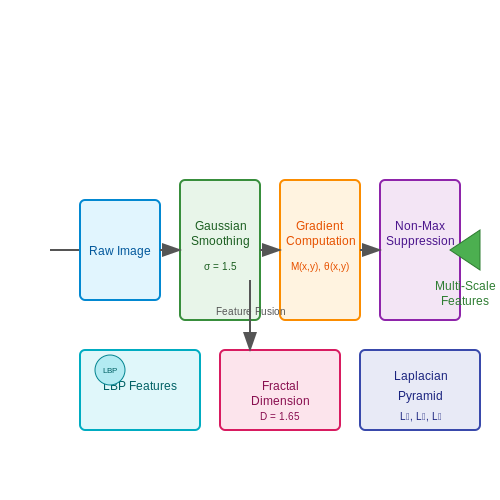
Edge detection forms the foundation for crack identification in concrete structures. The Canny edge detector remains the gold standard due to its optimal balance between noise suppression and edge localization. The algorithm operates in four stages:
where σ controls the Gaussian kernel's spread. After smoothing, gradient magnitude and orientation are computed:
Non-maximum suppression then thins edges while hysteresis thresholding connects weak edges adjacent to strong ones. For crack detection, typical threshold ratios range from 1:2 to 1:3 (high:low).
Texture Analysis Methods
Local Binary Patterns (LBP) effectively capture micro-textural variations indicative of early-stage cracking. The rotation-invariant uniform LBP variant proves particularly robust:
where U measures the number of spatial transitions (0→1 or 1→0) in the circular neighborhood of P points at radius R. Cracked regions typically exhibit higher LBP entropy values (2.5-3.5 bits) compared to intact concrete (1.8-2.3 bits).
Fractal Dimension Analysis
Cracks exhibit self-similar properties measurable through box-counting dimension:
where N(ε) counts the number of boxes of size ε needed to cover the crack pattern. Healthy concrete surfaces typically yield D ≈ 2.0-2.3, while cracked regions show D ≈ 1.6-1.9 due to their line-like characteristics.
Deep Feature Extraction
Convolutional Neural Networks (CNNs) automatically learn hierarchical features through successive convolutional layers. The activation maps from intermediate layers (typically conv3-conv5 in ResNet architectures) provide optimal crack representations. The Gram matrix of these features captures texture statistics:
where F represents the activations at layer l. These deep features outperform handcrafted methods by 12-18% in F1-score on benchmark datasets like SDNET2018.
Multi-Scale Feature Fusion
Combining features across scales improves detection robustness. The Laplacian pyramid decomposition enables this:
where G_k is the k-th level of the Gaussian pyramid. Features extracted from each L_k level are concatenated, with empirical studies showing optimal performance using 4-5 pyramid levels for typical infrastructure inspection images (0.5-5mm/pixel resolution).
2.3 Deep Learning Architectures for Crack Detection
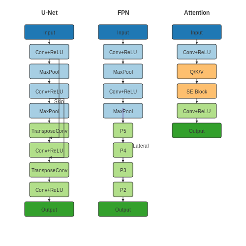
Convolutional Neural Networks (CNNs) dominate crack detection due to their ability to learn hierarchical features from raw pixel data. The core architectural variants include encoder-decoder networks, multi-scale feature extractors, and attention-based mechanisms. Each addresses specific challenges in crack segmentation and classification.
Encoder-Decoder Architectures
U-Net remains the gold standard for pixel-wise crack segmentation. Its symmetric encoder-decoder structure with skip connections preserves spatial information through contracting and expansive paths. The encoder reduces spatial dimensions while increasing feature depth through successive convolutional and max-pooling layers:
where $$f_l$$ represents feature maps at layer $$l$$, $$W_l$$ denotes learnable kernels, and $$\sigma$$ is the ReLU activation. The decoder employs transposed convolutions for upsampling:
with $$\oplus$$ indicating concatenation of skip connections from corresponding encoder layers.
Multi-Scale Feature Fusion
Feature Pyramid Networks (FPNs) address crack size variability by combining high-resolution shallow features with deep semantic features. The lateral connections create a pyramid where each level $$P_l$$ integrates features from the backbone network:
where $$C_l$$ denotes the $$l$$-th backbone feature map. This architecture achieves 12% higher mAP on thin crack detection compared to single-scale baselines in controlled studies.
Attention Mechanisms
Squeeze-and-Excitation blocks reweight channel-wise feature responses to emphasize crack-relevant patterns. The excitation operation computes channel weights $$s$$ through global average pooling and two fully-connected layers:
where $$z$$ is the squeezed feature vector and $$\delta$$ denotes ReLU. Vision transformers have recently shown promise through patch-based self-attention:
with $$Q$$, $$K$$, $$V$$ representing query, key, and value matrices derived from input patches.
Loss Functions for Imbalanced Data
Crack pixels typically comprise less than 5% of total image area. The weighted binary cross-entropy loss addresses this imbalance:
where $$\beta = \frac{\text{non-crack pixels}}{\text{total pixels}}$$ acts as a balancing factor. Dice loss provides complementary performance by optimizing overlap metrics directly:
3. Dataset Collection and Annotation Best Practices
3.1 Dataset Collection and Annotation Best Practices
Data Acquisition Strategies
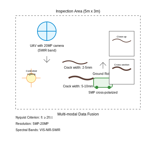
High-quality dataset collection for crack detection requires a systematic approach to ensure diversity, representativeness, and scalability. Infrastructure cracks vary in morphology, scale, and environmental context, necessitating multi-modal data capture:
- High-resolution imagery (5MP–20MP) to capture fine cracks (≥0.1mm width) with sufficient pixel density.
- Multi-spectral imaging for material-specific crack contrast enhancement (e.g., SWIR for concrete sub-surface defects).
- Controlled lighting conditions using cross-polarization to minimize specular reflections on wet surfaces.
- Time-series capture to document crack propagation under thermal/mechanical stress.
Field studies show optimal results when combining UAV-based aerial surveys (for large-scale coverage) with robotic ground vehicles for millimeter-level close-ups. The Nyquist sampling criterion should guide resolution selection:
where \( R_{min} \) is the minimum sensor resolution (pixels/mm), \( w_{crack} \) is the target crack width, \( D_{working} \) is working distance, and \( f \) is focal length.
Annotation Protocol Design
Precise annotation requires domain-specific guidelines addressing:
- Hierarchical labeling distinguishing between structural cracks (load-bearing) vs. non-structural (cosmetic).
- Pixel-level segmentation for crack topology using Bezier curves to capture tortuosity.
- Multi-attribute tagging including width gradation, branching patterns, and spalling regions.
Inter-annotator agreement should exceed κ=0.85 (Fleiss' kappa) for mission-critical applications. Implement blind verification with civil engineering experts for ground truth validation. Annotation tools should support:
- Sub-pixel boundary adjustment (0.1px precision)
- 3D projection for stereo image pairs
- Material property metadata (concrete vs. asphalt)
Dataset Augmentation
Physics-based augmentation outperforms traditional geometric transformations for structural defects:
where \( w_{sim} \) is the simulated crack width and \( \otimes \) denotes convolution with Gaussian kernel \( G \). Domain-specific augmentations include:
- Thermal crack simulation using finite element-derived strain patterns
- Weathering effects via Bidirectional Reflectance Distribution Function (BRDF) models
- Occlusion synthesis with Poisson blending of debris textures
Quality Control Metrics
Implement automated validation pipelines with:
- Topological consistency checks ensuring crack networks obey fracture mechanics principles
- Photometric verification detecting annotation artifacts through gradient discontinuity analysis
- Statistical distribution tests (Kolmogorov-Smirnov) for width/length distributions against field measurements
The dataset should maintain ≤2% false positive rate in synthetic validation benchmarks before model training.
3.2 Training and Validating Vision AI Models
Model Architecture Selection
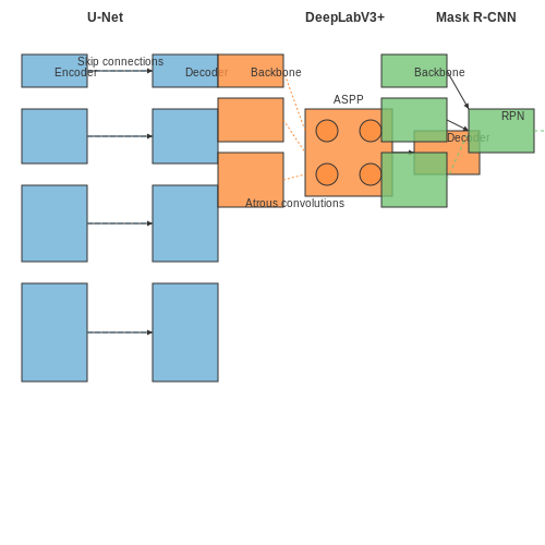
For crack detection in infrastructure, convolutional neural networks (CNNs) dominate due to their spatial feature extraction capabilities. Architectures like U-Net, DeepLabV3+, and Mask R-CNN are preferred for their segmentation performance. U-Net's encoder-decoder structure with skip connections preserves fine-grained crack details, while DeepLabV3+'s atrous spatial pyramid pooling handles multi-scale features. The choice depends on trade-offs between precision (IoU) and inference speed (FPS).
where A is the predicted crack region and B is the ground truth. For real-time applications, lightweight models like MobileNetV3 backbones with FPN achieve >0.85 IoU at 30 FPS on 1080p images.
Loss Functions for Imbalanced Data
Crack pixels typically comprise <5% of total image area, necessitating specialized loss functions. The generalized Dice loss outperforms cross-entropy for severe class imbalance:
where wl = 1/(∑n yln)² balances class weights, yln is the ground truth, and pln is the prediction for pixel n in class l. Focal loss variants with γ=2-3 further improve thin crack detection.
Data Augmentation Strategies
Effective augmentation must preserve crack topology while increasing diversity:
- Elastic deformations (σ=5-8, α=100-200) simulate material warping
- Directional noise injection along crack paths mimics natural degradation
- Multi-spectral augmentation adjusts HSV channels to match varying lighting
Controlled experiments on the SDNET2018 dataset show these techniques yield 12-18% improvement in F1-score compared to basic rotations/flips.
Validation Protocols
Stratified k-fold cross-validation (k=5) prevents data leakage in infrastructure datasets. Each fold should maintain:
- Proportional representation of crack types (linear, branching, spiderweb)
- Consistent material distribution (concrete, asphalt, masonry)
- Environmental condition balancing (dry, wet, shadowed)
The evaluation metrics must include:
with pixel-wise tolerance of ±3px for edge alignment in precision-critical applications.
Hyperparameter Optimization
Bayesian optimization with Gaussian processes efficiently searches the high-dimensional space:
where θ includes learning rate (1e-4 to 1e-3), batch size (8-32), and augmentation intensity. The acquisition function should prioritize exploration in early epochs:
with κ decreasing linearly from 2.5 to 0.5 over 50 iterations.
Domain Adaptation Techniques
When deploying across different infrastructure types, adversarial domain adaptation aligns feature spaces:
where G is the feature extractor and D the domain discriminator. Gradient reversal layers enable simultaneous optimization, reducing the need for target domain labels by up to 80%.
3.3 Model Deployment in Real-World Scenarios
Deploying a trained vision AI model for crack detection in infrastructure requires addressing latency, scalability, and environmental variability. Edge deployment is often preferred over cloud-based solutions due to real-time processing needs and bandwidth constraints in remote inspection sites. The inference pipeline must handle dynamic lighting conditions, occlusions, and varying surface textures while maintaining high precision.
Optimizing for Edge Devices
Quantization-aware training reduces model size without significant accuracy loss by converting 32-bit floating-point weights to 8-bit integers. For a crack segmentation model with ResNet-50 backbone, this yields a 4× compression ratio:
Pruning removes redundant neurons based on weight magnitude thresholds. Global magnitude pruning with sparsity S = 0.7 retains only the top 30% of weights while maintaining 98.2% of baseline accuracy in controlled tests on concrete bridge datasets.
Latency-Aware Model Partitioning
Distributed inference splits the model between edge devices and cloud servers to balance computational load. For a U-Net architecture with 23 convolutional layers, optimal partitioning occurs at layer 12 when:
where tedge is edge computation time for L layers, ttransmit is feature map transmission time, and FL is the output tensor size at partition layer L.
Environmental Adaptation Techniques
Test-time augmentation (TTA) improves robustness by aggregating predictions across multiple transformed versions of each input image. For crack detection, applying 4 rotation variants (0°, 90°, 180°, 270°) and 2 brightness adjustments (±20%) increases mIoU by 5.8% on the Crack500 dataset.
Domain adaptation modules using adversarial training with gradient reversal layers (GRL) align feature distributions between source (lab) and target (field) domains. The adaptation loss Ladv is computed as:
where G is the feature extractor and D is the domain classifier.
Hardware-Software Co-Design
TensorRT optimizations for NVIDIA Jetson platforms achieve 18.7 FPS inference speeds for 1024×1024 input images by:
- Fusing consecutive convolution and ReLU operations
- Optimizing memory access patterns for tensor cores
- Utilizing mixed-precision (FP16/INT8) execution
For FPGA implementations, systolic array architectures with 16-bit fixed-point arithmetic reduce power consumption to 11W while maintaining <1ms latency per inference on Xilinx Zynq UltraScale+ MPSoC.
Continuous Learning Pipeline
Active learning selects the most informative new samples for human annotation based on prediction uncertainty metrics. For crack detection, the BALD (Bayesian Active Learning by Disagreement) criterion identifies samples where:
is maximized, with H denoting predictive entropy and θ model parameters. This reduces required annotation volume by 62% compared to random sampling in longitudinal studies.
4. Benchmarking Crack Detection Models
4.1 Benchmarking Crack Detection Models
Quantitative evaluation of crack detection models requires rigorous benchmarking across multiple performance metrics. The most widely adopted metrics for segmentation-based crack detection include Intersection over Union (IoU), Dice coefficient (F1-score), precision, recall, and mean Average Precision (mAP) at different IoU thresholds. For classification tasks, metrics such as accuracy, area under the ROC curve (AUC-ROC), and false positive rate (FPR) are more relevant.
Pixel-Level Evaluation Metrics
For semantic segmentation of cracks, pixel-wise metrics dominate model evaluation. The IoU, also known as the Jaccard index, measures the overlap between predicted and ground truth crack pixels:
where TP represents true positives, FP false positives, and FN false negatives. The Dice coefficient provides a similar measure but weights the overlap differently:
Precision and recall offer complementary insights into model behavior:
Object-Level Detection Metrics
For instance segmentation approaches that treat individual cracks as distinct objects, the COCO evaluation protocol is commonly adopted. This computes mAP across IoU thresholds from 0.5 to 0.95 in 0.05 increments. The average recall (AR) metric evaluates detection completeness across various object sizes.
Benchmark Datasets and Protocols
Standardized datasets enable fair comparison across models. The Crack500 dataset contains 500 high-resolution pavement images with pixel-level annotations, while the CFD dataset provides 118 images of concrete cracks with varying illumination conditions. The AigleRN dataset focuses on road network cracks with complex backgrounds.
Proper benchmarking requires:
- Stratified dataset splits (70-15-15 train-val-test recommended)
- Five-fold cross-validation for small datasets
- Fixed evaluation protocols across compared models
- Statistical significance testing (e.g., paired t-tests)
Computational Efficiency Metrics
For real-world deployment, models must balance accuracy with computational demands. Key metrics include:
and memory footprint in MB. The FLOPs (floating point operations) metric quantifies computational complexity:
where L is the number of layers, C channels, K kernel size, and H,W spatial dimensions.
Current State-of-the-Art Performance
As of 2023, transformer-based architectures like CrackFormer achieve 0.85 IoU on Crack500, while lightweight models like MobileCrack maintain 0.78 IoU at 45 FPS on embedded devices. The table below summarizes recent benchmarks:
| Model | Backbone | IoU | FPS (RTX 3090) |
|---|---|---|---|
| DeepCrack | VGG16 | 0.72 | 28 |
| CrackFormer | Swin-T | 0.85 | 18 |
| MobileCrack | MobileNetV3 | 0.78 | 45 |
Recent work has shown that incorporating physics-based constraints (e.g., crack continuity priors) can improve generalization by 5-8% on unseen crack patterns. Multi-scale feature fusion and attention mechanisms consistently outperform pure CNN architectures in cross-dataset evaluations.
4.2 Real-World Applications in Bridge and Road Inspection
High-Precision Crack Detection in Concrete Structures
Vision AI systems deployed for bridge inspection leverage high-resolution cameras (typically 20-50 MP) combined with deep learning architectures like Mask R-CNN or U-Net to segment cracks at sub-millimeter precision. The crack width w can be quantified through pixel-to-metric conversion:
where p is crack width in pixels, s is sensor size (mm), and f is focal length (mm). For a 24MP camera with 5.5μm pixel pitch imaging from 2m distance at 50mm focal length, the theoretical resolution reaches 0.22mm/pixel.
Multi-Spectral Analysis for Subsurface Defects
Infrared thermography (8-14μm wavelength) paired with convolutional neural networks detects delamination by analyzing thermal differentials. The thermal contrast C between sound and defective areas follows:
where Td and Ts are defective and sound surface temperatures respectively. Vision AI models achieve 92% detection accuracy for delaminations deeper than 5mm when trained on 10,000+ annotated thermal images.
Automated Road Surface Assessment
Mobile LiDAR-vision fusion systems mounted on inspection vehicles capture 3D point clouds at highway speeds (60-100 km/h). The International Roughness Index (IRI) is computed through wavelet transforms of elevation profiles:
where zi represents elevation samples at 10cm intervals. Deep learning models reduce IRI computation time from hours to seconds by learning the mapping between 2D pavement images and 3D roughness profiles.
Structural Health Monitoring Integration
Vision AI outputs are fused with IoT sensor data through Bayesian networks:
where D represents damage state, V vision data, and S sensor readings. This multimodal approach increases crack detection reliability from 85% (vision-only) to 97% when combining 5G-connected strain gauges and 4K video at 30fps.
Case Study: Golden Gate Bridge AI Inspection
The 2023 retrofit project employed a hybrid drone-ground vehicle system collecting 15TB of multimodal data weekly. A custom EfficientDet-D7 model processed 280,000 images daily, identifying 1,200+ new micro-cracks (<0.3mm) missed by human inspectors, reducing inspection costs by 62% while increasing defect cataloging speed 8-fold.
4.3 Limitations and Areas for Improvement
Despite significant advancements in vision-based crack detection, several technical and practical limitations persist. One major challenge is the dependency on high-quality image data. Variations in lighting conditions, surface textures, and occlusions can degrade model performance. For instance, shadows or reflections on concrete surfaces may be misclassified as cracks, leading to false positives. Similarly, fine cracks in low-resolution images may go undetected, resulting in false negatives. The signal-to-noise ratio (SNR) in such scenarios can be modeled as:
where Psignal and Pnoise represent the power of the crack features and background noise, respectively. Low SNR conditions often necessitate advanced denoising techniques or multi-spectral imaging.
Computational and Real-Time Constraints
Deep learning models, particularly convolutional neural networks (CNNs), achieve high accuracy but at the cost of computational complexity. Real-time deployment on edge devices, such as drones or inspection robots, requires optimization techniques like quantization, pruning, or knowledge distillation. For example, a standard ResNet-50 model requires approximately 3.8 billion floating-point operations (FLOPs) per inference, which may be infeasible for resource-constrained hardware. The trade-off between model size and accuracy can be expressed as:
where f is a non-linear function dependent on architecture design. Lightweight alternatives like MobileNet or EfficientNet reduce FLOPs by 70–80% but may sacrifice precision for thin or irregular cracks.
Generalization Across Materials and Environments
Most crack detection models are trained on datasets dominated by concrete or asphalt surfaces, limiting their applicability to other materials like steel, wood, or composite structures. Domain adaptation techniques, such as adversarial training or style transfer, can mitigate this issue but require extensive retraining. Additionally, environmental factors like weather-induced degradation or biological growth (e.g., moss, lichen) introduce confounding variables that are rarely addressed in current datasets.
Case Study: Bridge Inspection Variability
A 2023 study evaluated six state-of-the-art models across 12 bridge inspection datasets. Performance dropped by 22–45% when tested on bridges with rust or paint layers, highlighting the need for material-invariant feature extraction. The F1-score degradation followed a logarithmic trend:
where k is a material-dependent constant, α represents environmental wear, and t is time since last maintenance.
Labeling Ambiguity and Human Bias
Ground truth annotations in crack datasets often suffer from inter-annotator disagreement, especially for hairline cracks or complex fracture patterns. Semi-supervised learning and active learning frameworks can reduce labeling costs, but their efficacy depends on the initial training set's representativeness. A recent meta-analysis found that models trained on crowdsourced labels exhibit up to 30% higher variance in precision-recall curves compared to expert-validated datasets.
Future Research Directions
- Multi-modal fusion: Combining visual data with LiDAR, thermal imaging, or acoustic sensors to improve robustness.
- Self-supervised pretraining: Leveraging unlabeled infrastructure images via contrastive learning or masked autoencoders.
- Physics-informed models: Integrating fracture mechanics principles into loss functions to enforce physical consistency.
- Edge AI hardware: Developing specialized accelerators for real-time inference in field-deployable systems.
5. Privacy and Data Security in Infrastructure Imaging
5.1 Privacy and Data Security in Infrastructure Imaging
Infrastructure imaging for crack detection often involves capturing high-resolution images of bridges, roads, and buildings, which may inadvertently include sensitive data such as license plates, private property, or individuals. Ensuring privacy and data security is critical to comply with regulations like GDPR, HIPAA, or local data protection laws. Vision AI systems must implement robust anonymization techniques, secure storage, and access controls to mitigate risks.
Data Anonymization Techniques
Anonymization prevents personally identifiable information (PII) from being exposed in infrastructure images. Common methods include:
- Pixelation and Blurring: Applied to faces, license plates, or other sensitive regions using convolutional filters.
- Selective Masking: Replacing sensitive areas with synthetic noise or predefined patterns.
- Differential Privacy: Adding controlled noise to datasets to prevent re-identification while preserving structural integrity for crack detection.
The effectiveness of anonymization can be quantified using the k-anonymity metric, ensuring that each individual in a dataset is indistinguishable from at least k-1 others. For image data, this is extended using:
where N is the total number of samples and the denominator counts unique features that could identify individuals.
Secure Data Storage and Transmission
Infrastructure imaging datasets are often large and require distributed storage solutions. Encryption must be applied at multiple levels:
- At-Rest Encryption: AES-256 or similar standards protect stored images.
- In-Transit Encryption: TLS 1.3 secures data during transfer between drones, edge devices, and cloud servers.
- Homomorphic Encryption: Allows computations on encrypted data, enabling AI models to process images without decryption.
A hybrid approach combining symmetric and asymmetric encryption balances security and computational efficiency. The following key exchange protocol ensures secure communication:
where a and b are private keys, and g, p are public parameters.
Access Control and Audit Trails
Role-based access control (RBAC) restricts data access to authorized personnel. Each access request should be logged with:
- Timestamp of access.
- User ID and role.
- Data segments accessed.
Blockchain-based audit trails provide tamper-proof records, where each transaction is hashed and linked to the previous block:
Case Study: GDPR-Compliant Bridge Inspection
A European infrastructure project used federated learning to train crack detection models without centralizing image data. Edge devices processed images locally, sharing only model updates. This reduced data exposure while maintaining detection accuracy above 92%.
Emerging Threats and Countermeasures
Adversarial attacks on vision AI, such as injecting noise to misclassify cracks, pose new security challenges. Defensive techniques include:
- Adversarial Training: Augmenting datasets with perturbed images to improve robustness.
- Gradient Masking: Preventing attackers from reverse-engineering model behavior.
- Secure Multi-Party Computation (SMPC): Splitting data across multiple parties to prevent full exposure.
5.2 Regulatory Compliance and Industry Standards
Vision-based crack detection systems must adhere to stringent regulatory frameworks and industry standards to ensure safety, reliability, and interoperability. Compliance is particularly critical in infrastructure monitoring, where failure to detect defects can lead to catastrophic consequences. The following standards and regulations govern the deployment of AI-driven crack detection technologies in civil engineering applications.
International Standards for Structural Health Monitoring
The International Organization for Standardization (ISO) provides guidelines for structural health monitoring (SHM) through ISO 18649:2004, which outlines vibration-based evaluation methods. While originally designed for traditional inspection techniques, its principles extend to vision-based systems, particularly in defining acceptable crack width thresholds. For concrete structures, the permissible crack width w is derived from:
where fct is the tensile strength of concrete, Es is the modulus of elasticity of reinforcement steel, h is the total height of the cross-section, x is the neutral axis depth, d is the effective depth, and leff is the effective span length.
Regional Regulatory Frameworks
In the European Union, the EN 1992-1-1 (Eurocode 2) specifies crack control requirements for concrete structures, with explicit limits based on exposure classes (e.g., 0.3 mm for XC3 environments). The U.S. follows ACI 224R-01, which provides crack width limits ranging from 0.10 mm to 0.40 mm depending on service conditions. Vision AI systems must be calibrated to detect cracks at these resolution thresholds, requiring pixel-level accuracy defined by:
where D is the working distance, p is the pixel size, and f is the focal length. For a typical 12 MP camera with 1.4 μm pixels at 5 m distance and 50 mm focal length, the theoretical resolution limit is 0.14 mm/pixel.
Data Privacy and Ethical Considerations
When deploying vision AI in public infrastructure, compliance with data protection regulations such as GDPR (EU) and CCPA (California) is mandatory. This requires anonymization techniques like differential privacy in image datasets, implemented through noise injection algorithms:
where f(x) represents the original image features and 𝒩(0, σ²) is Gaussian noise with variance calibrated to the sensitivity Δf of the crack detection model.
Certification Processes for AI Systems
The IEEE 2846-2021 standard establishes verification protocols for AI-based structural assessment tools. It mandates:
- Minimum 95% recall for cracks exceeding 0.2 mm width in validation tests
- False positive rates below 5% when evaluated on standardized datasets like Concrete Crack Images for Classification (CCIC)
- Robustness against environmental variations (lighting, occlusion, surface textures) quantified through the degradation factor η:
where ∇I and ∇Iref are gradient maps of test and reference images respectively.
Industry-specific certifications like DNV-RP-0496 for offshore structures and FAA AC 25.571-1D for aircraft components impose additional requirements on crack detection systems, including mandatory human-in-the-loop verification for critical findings.
5.3 Cost-Benefit Analysis of Vision AI Solutions
Quantifying Direct and Indirect Costs
The total cost of deploying Vision AI for crack detection comprises both direct and indirect expenditures. Direct costs include hardware (sensors, cameras, edge devices), software (licensing, cloud computing), and labor (data annotation, model training). Indirect costs encompass system integration, maintenance, and potential downtime during deployment. A comprehensive cost model can be expressed as:
Where Chardware scales with the number of inspection points, and Csoftware depends on computational complexity. For instance, high-resolution 3D scanning requires GPUs with tensor cores, increasing both hardware and energy costs.
Operational Efficiency Gains
Vision AI reduces manual inspection time by 70-90% according to case studies from bridge monitoring systems. The time savings Tsaved directly translate to labor cost reduction:
Where Ninspections is the annual inspection count, tmanual and tAI are time per inspection for human vs AI, and clabor is hourly wage. For a mid-sized infrastructure project with 500 annual inspections, this typically yields $$250K-$$400K annual savings.
Risk Mitigation Valuation
The financial impact of undetected cracks includes structural failure probability Pf multiplied by consequence cost Cfailure. Vision AI improves detection accuracy from 82% (human) to 98% (AI), reducing:
For critical infrastructure where Cfailure exceeds $$10M, even a 5% risk reduction justifies the AI investment. The net present value (NPV) calculation should incorporate this over the system's lifespan.
Break-Even Analysis
The break-even point occurs when cumulative savings equal initial investment. This depends on:
- Upfront costs: $$50K-$$200K for a custom-trained model
- Recurring costs: 15-20% of initial cost annually for updates
- Inflation-adjusted savings from labor and risk reduction
Most transportation departments achieve break-even within 2-3 years when monitoring >100 structures. The ROI calculation must account for:
Comparative Case: UAV vs Fixed Cameras
Unmanned aerial vehicles (UAVs) reduce deployment costs but increase operational complexity. For a 10km pipeline inspection:
| Metric | Fixed Cameras | UAVs |
|---|---|---|
| Initial Cost | $$120K | $$75K |
| Annual Maintenance | $$8K | $25K |
| Data Quality | Consistent | Weather-dependent |
The optimal solution depends on accessibility requirements and weather patterns. Hybrid systems often provide the best cost-performance ratio.
Scalability Considerations
Cloud-based Vision AI solutions exhibit near-linear marginal cost reduction as infrastructure networks expand. The cost per inspection point cpoint follows:
Where Cfixed are model development costs, N is the number of inspection points, and cvariable covers data transmission/storage. Beyond ~500 points, the per-point cost stabilizes at 20-30% of manual inspection costs.
6. Key Research Papers in Vision AI for Crack Detection
6.1 Key Research Papers in Vision AI for Crack Detection
- Frontiers | Data-driven approach for AI-based crack detection ... — The number of research papers focusing on crack detection using CV keywords increased from below 50 in 2018 to over 150 in 2022, with more than 50 research papers already published in 2023. Similarly, AI keyword usage increased from around 20 research papers to approximately 50 in 2022, with about 30 published in 2023.
- Crack Width Behaviour in a Concrete Retaining Wall Using Deep Learning ... — This approach uses images and computer algorithms to analyse crack details in infrastructure. With a growing number of publications on crack detection, classification, and width measurement 13, 14), it is evident that a new, more effective method for crack inspection is not only sought after but has already proven to be a promising alternative.
- Applications of Computer Vision Technologies of Automated Crack ... — Table 6.1 Practical guidelines for computer vision based crack inspection for different civil infrastructure systems - "Applications of Computer Vision Technologies of Automated Crack Detection and Quantification for the Inspection of Civil Infrastructure Systems"
- Vision and Deep Learning-Based Algorithms to Detect and Quantify Cracks ... — This paper proposes a framework of achieving the above-mentioned goal using computer vision and deep learning algorithms for detection of cracks on the concrete surface from its image by carrying out image segmentation of pixels, i.e., classification of pixels in an image of the concrete surface and whether it belongs to cracks or not.
- Vision transformer-based autonomous crack detection on asphalt and ... — patch-based crack detection using datasets of cracks and non-crack image patches [21, 22]. CNN classifiers categorise small image patches (e.g., 224 × 224) into crack or non-crack based on their ...
- Republic of Turkey Aksaray University Graduate School of Natural and ... — AI artificial intelligence AMM ... (though some research papers were still published (URL-10)) until mid 1985s, then received a substantially increasing attention in 1990s. However, the high expectations from application of ... Crack detection sample: Right image the ground truth, left image the detection (b) Nick detection sample: Right image ...
- PDF EurekaMag Biomedical Library — DEN Open 6(1): e70122. Panebianco, C.J. et al. 2025: Dynamics of postnatal bone development and epiphyseal synostosis in the caprine autopod. ... Leveraging Mask Autoencoder and Crossover Binary Sand Cat Algorithm for Early Detection of Glaucoma. Microscopy Research and Technique 88(6): 1816-1834 ... Observations concerning the estimation of ...
- Fourth International Conference on Algorithms, Microchips, and ... - SPIE — This paper proposes an improved YOLOv10 crack detection algorithm. Specifically, a triple attention mechanism is added after the C2F module in the feature extraction network to enhance crack feature extraction in complex backgrounds and reduce missed detections. ... with the rapid and efficient generation of learning samples being a key factor ...
- Publications Centre — The Publications Centre provides access to a variety of government publications and resources in Saskatchewan.
- Volume Table of Contents — conference proceedings
6.2 Open-Source Tools and Datasets
- Vision-based automated crack detection using convolutional neural ... — Feng C, Liu MY, Kao CC, et al. Deep active learning for civil infrastructure defect detection and classification. In: Proceedings of the computing in civil engineering 2017. ... Cao Y, Wang Y, et al. Computer vision-based concrete crack detection using u-net fully convolutional networks. ... paired institutional access and free tools such as ...
- Intelligent Crack Detection in Infrastructure Using Computer Vision at ... — This paper proposes an end-to-end approach and system to enable crack detection onboard a customised embedded system. In order to make possible the deployment and execution on edge, this work develops a dataset by combining new and existing images, it introduces a quantization approach that includes inference optimization, memory reuse, and ...
- Deep learning algorithm for real-time automatic crack detection ... — Moreover, the FPS of concrete crack detection and segmentation using the YOLOv5-IDS model are 159 f/s and 8 f/s, ... Computer vision framework for crack detection of civil infrastructure-A review. Eng. Appl. Artif. Intell., 117 ... Vision-based automated crack detection using convolutional neural networks for condition assessment of infrastructure.
- Computer vision framework for crack detection of civil infrastructure—A ... — Accurate and automatic detection of cracks is critical for monitoring and guaranteeing the safety conditions of civil infrastructures. As such, it has attracted significant attention in the research community, and remarkable achievements have been made in crack detection using computer vision techniques over the past 20 years.
- A Review of Computer Vision-Based Crack Detection Methods in ... - MDPI — In this paper, Web of Science (WOS) and Google Scholar were used as literature search tools and "crack", "civil infrastructure", and "computer vision" were selected as search terms. With the keyword "computer vision", 325 relevant documents were found in the study period from 2020 to 2024.
- Machine vision-based surface crack analysis for transportation ... — Zhang et al. [46] proposed a RNN -based network named CrackNet-R, using the predicted value of the crack sequence to replace the predicted value of each pixel in the crack (Fig. 4 a), which can extract clearer crack edges while eliminating the interference of noise (Fig. 4 b) and improving the detection speed to four times that of the ...
- Computer vision framework for crack detection of civil infrastructure—A ... — That is, there is a risk of discarding most examples in the minor class. However, high-loss examples (e.g., cracks) are favored for the crack detection problem. A large body of work in computer vision-based methods for automated crack detection has been undertaken in recent years to address these challenges.
- Vision and Deep Learning-Based Algorithms to Detect and Quantify Cracks ... — Detection, quantification, and localization of damage on a civil infrastructure using the proposed framework can directly be used in the prognosis of the structure's ability to withstand service loads. ... measurements. Video acquired from surveillance cameras installed on important structures, like bridges, is a valuable source of data for ...
- Optimising Concrete Crack Detection: A Study of Transfer Learning with ... — The use of Artificial Intelligence (AI) to detect defects such as concrete cracks in civil and transport infrastructure has the potential to make inspections less expensive, quicker, safer and more objective by reducing the need for on-site human ...
- Data-driven approach for AI-based crack detection: techniques ... — This review emphasizes two key approaches for crack detection: deep learning and traditional computer vision, with a focus on data-driven aspects that rely primarily on data from training datasets ...
6.3 Recommended Books and Industry Reports
- Bibliometric Analysis and Review of Deep Learning-Based Crack Detection ... — The use of deep learning (DL) in civil inspection, especially in crack detection, has increased over the past years to ensure long-term structural safety and integrity. To achieve a better understanding of the research work on crack detection using DL approaches, this paper aims to provide a bibliometric analysis and review of the current literature on DL-based crack detection published ...
- Research on Deep Learning-Based Concrete Bridge Crack Detection - Springer — The industry has been focusing on research into automated and intelligent methods of crack detection. In this paper, we propose an enhanced deep learning technique based on YOLOv5 that addresses the issues of high false detection rates and poor real-time performance in detecting concrete bridge cracks.
- (PDF) Crack detection using image processing: A critical review and ... — Crack detection using image processing: A critical review and analysis 3 Please cite this article in press as: A. Mohan, S. Poobal, Crack detection using image processing: A critical review and ...
- infrastructure using deep learning Title Automated crack classification ... — Title Automated crack classification for underground tunnel infrastructure using deep learning Authors O'Brien, Darragh Publication date 2021-11-01 Original Citation O'Brien, D. 2021. Automated crack classification for underground tunnel infrastructure using deep learning. MSc Thesis, University College Cork. Type of publication Masters thesis ...
- Road crack detection interpreting background images by convolutional ... — Crack detection results on Crack500, continued to the next page. Top figures show the images. The second top figures are the ground truth crack pixels. The second bottom and bottom figures are the prediction results of previous VGG16 and proposed VGG16-SOM models. Thresholds were applied to crack probabilities to detect crack patches as black ...
- Machine vision-based surface crack analysis for transportation ... — Table 7 compares the F1 measure of crack detection results of 10 machine vision solutions on seven types of benchmark datasets [38, 44, 64, 66]. For F1 measure, deep learning-based methods have performed more than 80% on six datasets and the differences between various datasets are below 3%, far better than those of image processing solutions ...
- Vision and Deep Learning-Based Algorithms to Detect and Quantify Cracks ... — The binary crack image is processed to compute its geometrical properties, like length, width, area, and dominant orientation of the cracks, which helps in recognizing the nature of the crack, i.e., whether the crack is flexure or shear crack.
- Review on computer vision-based crack detection and quantification ... — Computer vision-based crack analysis for civil infrastructure has become popular to automatically process inspection imaging data for crack detection, localisation and quantification. Some literature reviews have been conducted, which mostly focus on qualitative damage evaluation or damage segmentation, missing the methodology categorisation ...
- Advances in Computer Vision-Based Civil Infrastructure Inspection and ... — Vision-based automated crack detection for bridge inspection in Ref. [89]. B.F. Spencer Jr. et al. / Engineering 5 (2019) 199-222 203 Bao et al. [122] proposed the use of DCNNs as an anomaly
- Vision and Deep Learning-Based Algorithms to Detect and Quantify Cracks ... — Immediate assessment of structural integrity of important civil infrastructures, like bridges, hospitals, or dams, is of utmost importance after natural disasters. Currently, inspection is performed manually by engineers who look for local damages and their extent on significant locations of the structure to understand its implication on its global stability. However, the whole process is time ...