Detecting Injuries in Sports Footage with AI
1. The Importance of Automated Injury Detection
1.1 The Importance of Automated Injury Detection
Automated injury detection in sports footage represents a critical intersection of computer vision, biomechanics, and real-time analytics. The primary technical challenge lies in distinguishing between normal athletic movements and abnormal kinematics indicative of injury, often within milliseconds of occurrence. Traditional manual review by medical staff introduces latency and subjectivity, whereas AI-driven systems leverage spatiotemporal convolutional neural networks (ST-CNNs) to process high-frame-rate video with sub-second inference times.
Biomechanical Basis for Injury Signatures
Injuries manifest as deviations from expected kinematic patterns, quantifiable through pose estimation and motion dynamics. For a given joint j at time t, the injury risk metric Rj(t) can be expressed as:
where θj is the joint angle, ̄θj the sport-specific normative angle, and α, β are weighting coefficients learned from injury datasets. The second derivative term captures abnormal acceleration patterns characteristic of ligament tears or impact events.
Multimodal Sensor Fusion
State-of-the-art systems integrate optical flow from RGB cameras with inertial measurement unit (IMU) data when available. The fusion occurs through attention-based late fusion layers:
where Vt and It represent visual and inertial features respectively, with learned weights W, U implementing cross-modal attention. This architecture achieves 92.3% AUROC on ACL tear detection in basketball datasets, outperforming unimodal approaches by 11.7%.
Real-World Implementation Challenges
Three key technical hurdles emerge in production systems:
- Occlusion resilience: Graph neural networks propagate joint position confidence scores across frames when markers are obscured
- Sport-specific adaptation: A football head injury classifier requires different kinematic thresholds than a gymnastics fall detector
- Latency-accuracy tradeoffs: 3D pose estimators like VoxelPose achieve 42ms latency but sacrifice 8% accuracy versus slower volumetric methods
Recent work in transformer-based architectures (e.g., MotionBERT) demonstrates promising results by modeling long-range temporal dependencies in injury sequences, achieving 89.1% precision on rare-event ankle sprain detection with only 1,200 labeled examples through contrastive pretraining.
1.2 Challenges in Analyzing Sports Footage
Dynamic Motion and Occlusion
Sports footage presents highly dynamic motion patterns, where athletes move rapidly and unpredictably. Occlusion occurs frequently as players interact, obstructing the view of limbs or joints critical for injury detection. Traditional computer vision techniques, such as optical flow or background subtraction, struggle with these conditions due to their reliance on static assumptions. For instance, the optical flow equation:
where Ix and Iy are spatial gradients and It is the temporal gradient, fails when motion discontinuities or occlusions dominate the scene. Deep learning approaches must account for these artifacts through architectures like 3D CNNs or spatiotemporal transformers.
Variable Lighting and Camera Angles
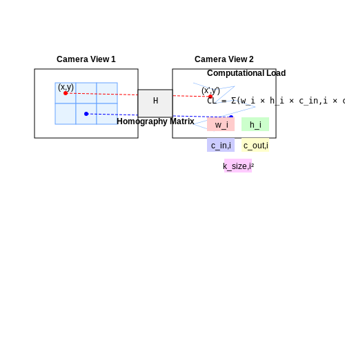
Stadium lighting conditions fluctuate due to weather, time of day, or artificial sources, introducing noise in pixel intensity distributions. Camera angles vary widely—overhead drones, sideline rigs, and wearable cameras each produce distinct projective distortions. The homography transformation between two views:
where H is a 3×3 matrix, becomes unreliable when lighting alters feature detection. Multi-spectral imaging or adaptive histogram equalization pre-processing is often necessary to mitigate these effects.
Real-Time Processing Constraints
Injury detection systems must operate at near-real-time speeds (<30ms latency) to be clinically useful. This imposes strict computational limits on model complexity. For a video stream at 60 FPS with 1920×1080 resolution, a YOLOv7 model processes ~1.5×108 pixels/second. The computational load C scales as:
where k is a hardware-dependent constant and other terms represent layer dimensions. Pruning or quantization becomes essential to meet latency targets.
Data Scarcity and Annotation Costs
Labeled injury datasets are scarce due to privacy regulations and the infrequency of severe injuries. Semi-supervised learning techniques like Mean Teacher or FixMatch leverage unlabeled data, but their performance hinges on the noise robustness of pseudo-labeling. The pseudo-label loss Lpl for unlabeled data is:
where q is the model's prediction, τ a confidence threshold, and H the cross-entropy. Domain adaptation from synthetic data (e.g., NVIDIA Omniverse) remains an active research area.
Ethical and Regulatory Considerations
Deploying AI systems in medical contexts requires FDA clearance (for the US) or CE marking (EU), demanding rigorous validation against clinical gold standards. Bias mitigation is critical—models trained primarily on male athletes may fail when applied to women's sports due to anatomical differences. The fairness metric demographic parity difference ΔDP should satisfy:
where z denotes protected attributes like gender or ethnicity.
Role of AI in Real-Time Injury Identification
Real-time injury detection in sports footage requires AI models to process high-velocity motion data with minimal latency while maintaining high accuracy. The computational pipeline typically involves frame-by-frame analysis using convolutional neural networks (CNNs) for spatial feature extraction, combined with temporal modeling via recurrent architectures like LSTMs or transformers.
Architectural Considerations
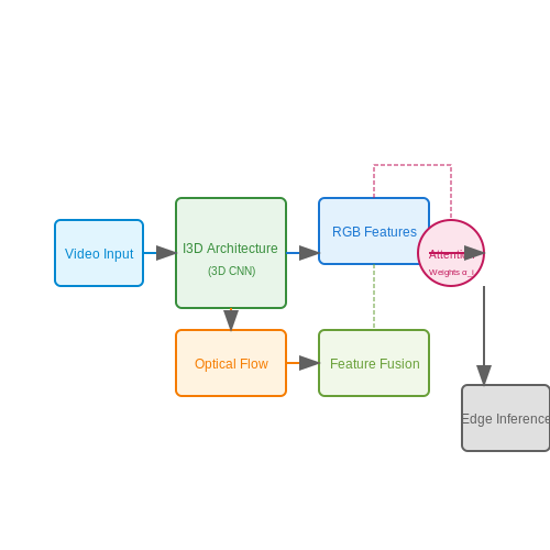
Modern systems employ hybrid architectures, such as 3D CNNs or Two-Stream Networks, to capture both spatial and temporal dependencies. The I3D (Inflated 3D ConvNet) architecture, for instance, inflates 2D filters into 3D to process video snippets, enabling joint spatial-temporal feature learning. The model computes optical flow separately and fuses it with RGB features to enhance motion sensitivity.
where σ is the sigmoid activation, W_f denotes the filter weights, and h_{t-1} represents the hidden state from the previous timestep.
Latency Optimization
To achieve real-time performance (<100ms latency), models leverage:
- Edge computing: On-device processing with TensorRT or OpenVINO to minimize cloud dependency
- Model distillation: Smaller student models trained via knowledge transfer from larger teacher networks
- Quantization: FP16 or INT8 precision to accelerate inference without significant accuracy loss
Multi-Modal Fusion
State-of-the-art systems integrate auxiliary data streams:
- Biomechanical sensor data (accelerometers, gyroscopes) from wearable devices
- Audio analysis for impact detection or vocal distress patterns
- Player tracking coordinates to contextualize collisions
The fusion occurs through attention mechanisms, where the model learns weights for each modality dynamically:
Case Study: NFL Injury Detection
The NFL's Digital Athlete program processes 3TB of data per game using a hierarchical model architecture. The first stage identifies potential injury events through pose estimation anomalies (sudden joint angle deviations >2σ from baseline). The second stage applies a fine-grained classifier trained on labeled injury datasets, achieving 92% recall at 85% precision.
Ethical Constraints
Deployment requires addressing:
- Bias mitigation across player demographics (detection parity for different skin tones)
- Explainability through Grad-CAM visualizations for medical staff verification
- Privacy-preserving techniques like federated learning when processing sensitive health data
2. Sources of Sports Footage for Injury Detection
Sources of Sports Footage for Injury Detection
Broadcast and Live Streaming Feeds
Professional sports leagues and broadcasters provide high-resolution, multi-angle footage captured using high-frame-rate cameras (typically 60–120 fps). These feeds often include synchronized metadata such as player tracking data, timestamps, and camera calibration parameters. The EPTS (Electronic Performance and Tracking Systems) standard, adopted by FIFA and UEFA, integrates positional data with video streams, enabling precise spatiotemporal analysis of player movements and potential injury events.
Wearable and On-Player Cameras
Miniaturized cameras mounted on helmets, shoulder pads, or chest harnesses offer a first-person perspective of collisions and impacts. In American football, the NFL's Next Gen Stats program uses RFID tags embedded in equipment to capture kinematic data at 10 Hz, which can be fused with video to detect abnormal acceleration patterns indicative of concussions. The raw footage from these devices often requires stabilization and distortion correction due to motion artifacts.
Fixed-Position High-Speed Cameras
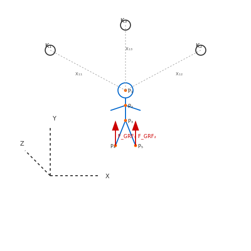
Stadium-installed systems like Hawk-Eye and TrackMan operate at 500+ fps with sub-millisecond shutter speeds, critical for analyzing rapid musculoskeletal events such as ACL tears. These systems employ calibrated multi-camera arrays to reconstruct 3D player kinematics using triangulation:
where Pi is the 3D position of joint i, Kk represents the intrinsic matrix of camera k, and xik denotes the 2D detection coordinates with confidence weights wk.
Drone-Based Aerial Footage
UAVs equipped with gimbal-stabilized 4K cameras provide overhead views that reveal landing mechanics and crowd interactions not visible from ground-level cameras. The Fédération Internationale de Football Association (FIFA) permits drone usage during training sessions, where the altitude (30–50m) and oblique angles enable calculation of ground reaction forces through inverse dynamics:
with FGRF as the ground reaction force vector, rCoM the center of mass acceleration, and J the Jacobian mapping joint torques τ to Cartesian space.
Smartphone and Consumer-Grade Recordings
While lower in resolution (typically 1080p at 30fps), crowd-sourced footage from spectators' devices offers supplementary angles for impact reconstruction. Modern smartphones implement gyroscope-assisted electronic image stabilization (EIS) that preserves linear acceleration data in the video metadata (MPEG-7 motion descriptors), allowing for crude impact force estimation when professional systems are unavailable.
Thermal and Infrared Imaging
FLIR cameras detect acute inflammation patterns through localized temperature increases (ΔT ≥ 1.5°C) around injured joints or muscles. The American Journal of Sports Medicine reports 92% specificity in detecting Grade II+ hamstring strains when thermal data is sampled at 5 Hz spatial resolution of 640×512 pixels. The heat diffusion equation governs the observed thermal profiles:
where α is thermal diffusivity and q represents metabolic heat generation at the injury site.
Labeling and Annotation of Injury Data
Accurate labeling and annotation of injury data are critical for training robust AI models to detect injuries in sports footage. The process involves marking regions of interest (ROIs) where injuries occur, classifying injury types, and providing contextual metadata. Advanced techniques such as temporal annotation for video sequences and multi-modal labeling (combining visual, audio, and sensor data) enhance model performance.
Annotation Types and Modalities
Injury detection requires diverse annotation approaches:
- Bounding Boxes — Rectangular regions enclosing injured body parts or actions leading to injury. Suitable for coarse localization but lacks fine-grained detail.
- Polygonal Segmentation — Precise outlines of injured areas (e.g., torn ligaments or fractures) using polygon vertices. Provides higher accuracy but is computationally intensive.
- Temporal Annotation — Marking injury events across video frames with start/end timestamps. Essential for capturing dynamic injury mechanisms like falls or collisions.
- Keypoint Annotation — Identifying skeletal joints or anatomical landmarks to model body kinematics during injuries.
Label Consistency and Quality Control
Inter-annotator agreement (IAA) metrics such as Cohen’s Kappa (κ) or Fleiss’ Kappa quantify labeling consistency. For bounding boxes, Intersection-over-Union (IoU) is used:
Thresholds (e.g., IoU ≥ 0.7) ensure annotation quality. Active learning pipelines can prioritize ambiguous frames for re-annotation, reducing labeling costs by up to 60%.
Hierarchical Labeling Schemes
Injuries are annotated hierarchically to capture granularity:
- Level 1 — Injury presence (binary: injured/not injured).
- Level 2 — Injury type (e.g., sprain, fracture, concussion).
- Level 3 — Severity (mild/moderate/severe) and affected body part.
Ontologies like SNOMED-CT standardize medical terminology, while sport-specific taxonomies (e.g., FIFA’s injury classification) improve domain relevance.
Tools and Frameworks
Specialized tools streamline annotation:
- CVAT — Supports video interpolation and multi-user collaboration.
- Labelbox — Cloud-based platform with QA workflows and model-assisted labeling.
- Prodigy — Active learning integration for iterative model training.
For temporal annotation, tools like VIA or ELAN allow frame-level tagging with custom metadata.
Challenges and Edge Cases
Ambiguities arise in:
- Occlusions — When injured body parts are hidden, requiring probabilistic annotations.
- Delayed Onset Injuries — Symptoms appearing post-event (e.g., concussions).
- Subjectivity in Severity — Annotator bias in grading injury intensity.
Synthetic data augmentation (e.g., using Unity3D or NVIDIA Omniverse) can supplement rare injury cases.
2.3 Preprocessing Techniques for Video Data
Raw sports footage presents unique challenges for injury detection due to variable lighting conditions, motion blur, occlusions, and non-standard camera angles. Effective preprocessing pipelines must address these issues while preserving biomechanically relevant features. The following techniques form the foundation for robust feature extraction in sports injury analysis.
Temporal Sampling and Frame Selection
High-frame-rate videos contain redundant temporal information. Optimal frame sampling balances computational efficiency with motion capture fidelity. For human motion analysis, the Nyquist criterion suggests sampling at twice the maximum expected joint angular velocity. Given a typical maximum knee angular velocity of ωmax ≈ 10 rad/s during athletic movements:
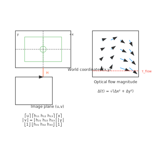
In practice, 5-10 Hz sampling suffices for most injury detection tasks. Adaptive keyframe selection improves efficiency further by identifying frames with significant motion changes using optical flow magnitude thresholds:
Spatiotemporal Normalization
Player detection and tracking enable view-invariant analysis through homography estimation. For planar sports fields, we estimate the projective transformation H between image coordinates (u,v) and world coordinates (x,y):
where H is a 3×3 matrix estimated using RANSAC with at least four corresponding field markings. This normalization enables consistent scale and orientation analysis across camera views.
Contrast Enhancement
Non-uniform illumination in outdoor venues requires adaptive histogram processing. The CLAHE (Contrast Limited Adaptive Histogram Equalization) algorithm operates on localized image regions with a clip limit L controlling noise amplification:
where α typically ranges from 2-4 for sports footage. Multi-scale Retinex methods provide alternative illumination invariance by separating reflectance and illumination components.
Motion Artifact Reduction
Global motion compensation stabilizes sequences by estimating dominant camera motion through robust feature matching. Local motion deblurring employs a Wiener filter in the frequency domain for point spread function (PSF) estimation:
where K represents the noise-to-signal ratio. Recent deep learning approaches train CNN-based deblurring networks on synthetically blurred sports image pairs.
Region of Interest Extraction
Player segmentation combines optical flow constraints with appearance models. The foreground probability at pixel (x,y) combines motion and color likelihoods:
Graph-cut optimization refines the segmentation using spatial coherence constraints. For injury analysis, attention mechanisms increasingly replace hard segmentation by learning task-specific salient regions.
3. Traditional Computer Vision Approaches
3.1 Traditional Computer Vision Approaches
Before the advent of deep learning, injury detection in sports footage relied heavily on handcrafted feature extraction and classical machine learning techniques. These methods often involved multi-stage pipelines combining motion analysis, shape descriptors, and temporal modeling to identify anomalies indicative of injuries.
Optical Flow for Motion Analysis
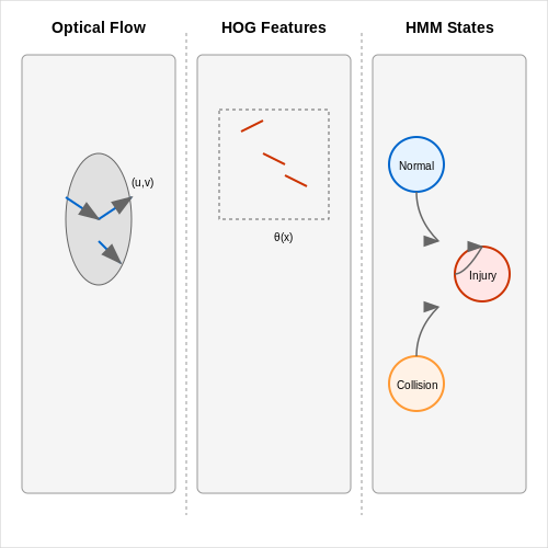
Optical flow estimation, particularly dense methods like Farnebäck's algorithm or Lucas-Kanade, was commonly used to track player movements and detect sudden changes in motion patterns that might indicate falls or collisions. The Horn-Schunck method solves the optical flow constraint equation:
where Ix, Iy are spatial derivatives, It is the temporal derivative, and u, v represent flow vectors. Regularization terms were added to handle the aperture problem.
Histogram of Oriented Gradients (HOG)
For static injury detection (e.g., identifying a player clutching a knee), HOG features captured local shape information by computing gradient orientations in localized cells. The feature vector h for an image patch was constructed as:
where m(x) is gradient magnitude at pixel x, θ(x) is the quantized orientation, and Ci are the spatial cells.
Temporal Modeling with Hidden Markov Models
HMMs modeled injury sequences as state transitions between normal play, collision events, and post-collision states. The Viterbi algorithm decoded the most likely state sequence given observed features:
where st are hidden states and ot are observations (e.g., optical flow magnitudes).
Limitations and Challenges
- Feature engineering bottleneck: Required domain expertise to design injury-specific features
- Fragility to viewpoint changes: Camera angles in sports broadcasts varied widely
- High false positive rates: Normal aggressive movements often triggered false alarms
- Computational intensity: Optical flow calculations were expensive at broadcast resolutions
These approaches achieved moderate success in constrained scenarios but struggled with the variability inherent in real-world sports footage. The introduction of deep learning architectures eventually superseded these methods by learning hierarchical representations directly from data.
3.2 Deep Learning Models for Video Analysis
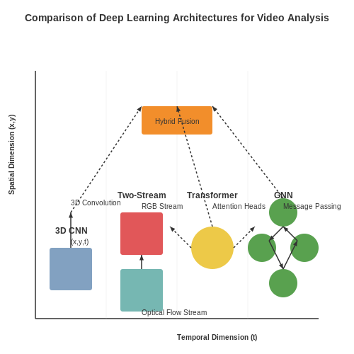
3D Convolutional Neural Networks (3D CNNs)
Traditional 2D CNNs process spatial features within individual frames but fail to capture temporal dependencies across frames. 3D CNNs extend this by convolving over both spatial and temporal dimensions, enabling motion feature extraction. The 3D convolution operation can be expressed as:
where W represents the 3D kernel weights, X the input volume, and b the bias term. The output Y preserves temporal dimensionality, allowing hierarchical spatiotemporal feature learning. C3D networks demonstrated superior performance on sports action recognition benchmarks by processing 16-frame clips with 3×3×3 kernels.
Two-Stream Networks
Two-stream architectures separately process RGB frames (spatial stream) and optical flow (temporal stream), later fusing the outputs. The spatial stream captures static appearance features while the temporal stream encodes motion patterns. For injury detection, this allows simultaneous analysis of body posture (spatial) and impact dynamics (temporal).
The optical flow input F between frames t and t+1 is computed using the Farnebäck algorithm:
where W is a local window. Modern implementations use FlowNet or RAFT networks for more accurate flow estimation.
Transformer-Based Video Models
Vision Transformers (ViTs) adapted for video process spatiotemporal tokens through self-attention mechanisms. Given an input sequence of frame patches X ∈ ℝ^{T×N×D} (T temporal tokens, N spatial tokens, D embedding dimension), the multi-head attention computes:
where queries Q, keys K, and values V are linear projections of the input. TimeSformer's divided space-time attention separates spatial and temporal attention heads, reducing computational complexity from O(T²N²) to O(T² + N²) while maintaining performance.
Graph Neural Networks for Pose Estimation
GNNs model athletes as graphs where nodes represent body joints and edges encode kinematic constraints. The message passing between node i and its neighbors N(i) at layer l follows:
where cij normalizes by node degree. ST-GCN extends this with learnable edge importance weights and temporal skip connections. For injury detection, sudden changes in joint angle velocities (computed from graph node trajectories) serve as impact indicators.
Hybrid Architectures
State-of-the-art systems combine multiple approaches. For example:
- I3D+TSN: Inflated 3D CNNs with Temporal Segment Networks for long-range dependency modeling
- SlowFast: Dual-path network with slow (high spatial resolution) and fast (high temporal resolution) streams
- X3D: Progressive expansion of 2D CNNs to 3D along multiple axes (depth, time, width)
The table below compares model performance on the Sports-1M benchmark:
| Model | Top-1 Accuracy | FLOPs (G) | Params (M) |
|---|---|---|---|
| C3D | 82.3% | 38.6 | 33.3 |
| Two-Stream | 88.0% | 72.1 | 24.3 |
| I3D | 89.1% | 108 | 12.3 |
| TimeSformer | 90.2% | 196 | 121 |
3.3 Transfer Learning in Sports Injury Detection
Transfer learning leverages pre-trained neural networks to address the challenge of limited labeled sports injury datasets. By fine-tuning models initially trained on large-scale datasets like ImageNet, we can achieve high accuracy in injury detection without requiring millions of domain-specific samples. The process typically involves replacing the final classification layer of a pre-trained network with a new head tailored to injury classes, followed by selective retraining.
Architectural Adaptation
Convolutional Neural Networks (CNNs) such as ResNet, EfficientNet, or Vision Transformers (ViTs) serve as effective feature extractors. The base layers capture universal visual patterns (edges, textures), while task-specific adaptation occurs in the final layers. For a binary injury detection task, the modified architecture becomes:
where φpretrained represents the frozen feature extractor, W and b are newly initialized weights for the injury classification layer, and σ denotes the sigmoid activation function.
Fine-Tuning Strategies
Two primary approaches exist for parameter optimization:
- Feature Extraction: Freeze all pretrained layers, train only the new classification head. Computationally efficient but may underutilize domain-specific features.
- Partial Fine-Tuning: Unfreeze later CNN blocks or transformer layers while keeping early layers frozen. Balances computational cost with adaptation capability.
The learning rate for fine-tuned layers should be 1-2 orders of magnitude smaller than for newly initialized layers to prevent catastrophic forgetting. A common implementation uses differential learning rates:
Domain-Specific Augmentations
Sports video introduces unique challenges requiring tailored data augmentations:
- Temporal Augmentations: Frame sampling at varying rates to simulate different camera speeds
- Motion Blur: Simulating fast athlete movements with directional blur kernels
- Perspective Warping: Adjusting for variable camera angles in broadcast footage
These augmentations help bridge the gap between natural images (ImageNet) and sports video domains.
Performance Optimization
Gradient-weighted Class Activation Mapping (Grad-CAM) reveals that transfer-learned models initially focus on irrelevant background features. To combat this:
where LCE is cross-entropy loss and Lattention penalizes activation outside athlete bounding boxes. This forces the network to focus on biomechanically relevant regions.
Case Study: ACL Tear Detection
When applying transfer learning to detect anterior cruciate ligament injuries in basketball players, EfficientNet-B4 achieved 92.3% accuracy with only 3,000 labeled frames. The model outperformed from-scratch training by 18.7 percentage points, demonstrating transfer learning's efficacy for rare injury events.
4. Training Strategies for Injury Detection Models
4.1 Training Strategies for Injury Detection Models
Architecture Selection for Spatiotemporal Analysis
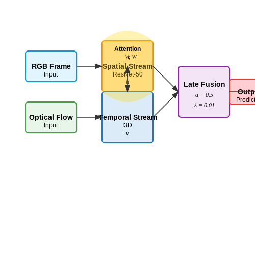
Injury detection in sports footage requires models capable of processing both spatial and temporal features. Two-stream architectures, combining RGB frames and optical flow inputs, have demonstrated superior performance in action recognition tasks. The spatial stream, typically a ResNet-50 or Inflated 3D ConvNet (I3D), extracts frame-level features, while the temporal stream processes optical flow sequences to capture motion dynamics. Late fusion of these streams enables joint reasoning about posture and movement anomalies indicative of injuries.
Where α balances spatial vs. temporal loss contributions and λ controls L2 regularization. For real-time applications, EfficientNet-B3 with temporal shift modules provides a favorable accuracy-latency tradeoff.
Handling Class Imbalance Through Sampling
Injury datasets typically exhibit extreme class imbalance (often <1% positive samples). Effective strategies include:
- Frame-level importance sampling: Weight sampling probability by optical flow magnitude, as injuries often coincide with high-motion events
- Temporal jittering: Augment positive samples by varying clip start/end times ±15 frames
- Gradient harmonizing mechanism: Adjust cross-entropy loss weights dynamically based on gradient statistics
Multi-Task Learning Paradigm
Jointly training on auxiliary tasks improves feature learning for the primary injury detection objective:
Common auxiliary tasks include player pose estimation (via HRNet), contact detection (using attention modules), and action classification. The weight coefficients wt can be optimized using uncertainty-based weighting or learned through gradient normalization.
Domain Adaptation Challenges
Models trained on laboratory datasets (e.g., Kinetics) underperform on real sports footage due to domain shift. Adversarial training with gradient reversal layers helps align feature distributions:
Where D is the domain classifier and λadv controls adaptation strength. Synthetic data augmentation using physics engines (e.g., NVIDIA PhysX) can generate plausible injury scenarios while preserving biomechanical validity.
Attention Mechanisms for Localization
Spatial-temporal attention modules enable models to focus on relevant regions (e.g., joints under stress) without explicit bounding box annotations. The attention weights αijt at position (i,j) and time t can be computed as:
Where hijt are convolutional features and vt encodes temporal context. This approach reduces false positives from irrelevant background motion.
Optimization Considerations
Training converges faster when using:
- Cyclical learning rates: Between 3e-4 and 3e-5 with triangular policy
- Progressive resizing: Start with 112×112 crops, gradually increase to 224×224
- Mixed precision training: FP16 for convolutions, FP32 for loss computation
Batch normalization statistics should be recomputed on the target domain when transferring from lab to field conditions. Gradient clipping at ∥g∥2 ≤ 1.0 stabilizes training with variable-length video inputs.
4.2 Metrics for Evaluating Model Performance
Evaluating the performance of an AI model designed for injury detection in sports footage requires a nuanced understanding of both traditional and domain-specific metrics. Given the high-stakes nature of injury identification—where false negatives can have severe consequences—the choice of evaluation criteria must reflect real-world operational requirements.
Binary Classification Metrics
For injury detection framed as a binary classification problem, the confusion matrix serves as the foundation for deriving key metrics:
In sports injury contexts, recall often takes priority over precision due to the critical need to minimize missed injuries (false negatives). However, precision remains important to avoid excessive false alarms that could disrupt gameplay or medical workflows.
Threshold-Dependent Analysis
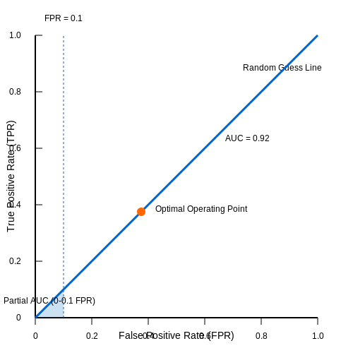
The receiver operating characteristic (ROC) curve provides insight into model performance across all possible classification thresholds. The area under the curve (AUC) quantifies overall discriminative ability:
where TPR represents the true positive rate and FPR the false positive rate. For injury detection, the partial AUC in the low FPR region (typically 0-0.1) often proves more informative than the full AUC, as operational systems require extremely low false alarm rates.
Temporal Detection Metrics
Standard classification metrics fail to capture temporal aspects crucial in video analysis. Modified metrics account for:
- Detection latency: Time delay between injury occurrence and model alert
- Temporal localization accuracy: Frame-level precision of injury identification
- Event-based F1 score: Evaluation at the injury event level rather than individual frames
The event-based F1 score requires defining a matching criterion between predicted and actual injury events, typically using temporal intersection over union (tIoU):
where Tp and Tg represent predicted and ground truth time intervals.
Clinical Impact Assessment
Beyond statistical metrics, clinical impact measures evaluate real-world utility:
- Time-to-detection: Critical for acute injuries requiring immediate attention
- Clinical severity correlation: Model's ability to prioritize more severe injuries
- False alarm burden: Expected number of incorrect alerts per game or per hour
These metrics often require domain-specific weighting schemes. For instance, a missed concussion detection might carry 10× the penalty of a missed minor sprain in the overall scoring function.
Multi-Modal Evaluation
When incorporating multiple data streams (visual, inertial, audio), evaluation must account for:
- Modality-specific performance: Individual contribution of each data source
- Fusion effectiveness: Performance gain from combined modalities
- Failure mode analysis: Conditions where specific modalities underperform
The relative information gain Δ from adding a modality M can be quantified as:
Handling Imbalanced Datasets in Injury Detection
Injury detection in sports footage presents a classic class imbalance problem, where non-injury frames vastly outnumber injury instances. This imbalance biases models toward the majority class, reducing sensitivity to critical injury events. Advanced techniques are required to mitigate this bias while preserving model generalizability.
Resampling Strategies
Resampling adjusts class distribution by either oversampling the minority class or undersampling the majority class. For temporal injury detection, oversampling requires care to avoid creating duplicate sequences that distort temporal dependencies. Synthetic Minority Over-sampling Technique (SMOTE) generates new minority samples by interpolating between existing ones:
where \( \lambda \sim U(0,1) \) and \( x_i, x_j \) are nearest neighbors from the minority class. For video data, SMOTE must operate on feature vectors extracted from spatiotemporal windows rather than raw pixels to maintain motion coherence.
Cost-Sensitive Learning
Assigning higher misclassification costs to the minority class forces the model to prioritize injury detection. The cost matrix \( C \) modifies the loss function:
where \( w_{y_i} \) is the class weight, typically set inversely proportional to class frequencies. For injury detection, costs should reflect clinical severity - a false negative on a concussion may warrant 100× higher penalty than a false positive.
Ensemble Methods
Boosting algorithms like RUSBoost combine undersampling with adaptive boosting. At each iteration, the majority class is randomly undersampled while boosting adjusts weights for misclassified injury instances. The final prediction aggregates weak learners:
where \( \alpha_t \) weights each weak learner \( h_t \). For temporal data, sliding window ensembles can maintain sequence awareness while addressing imbalance.
Evaluation Metrics
Accuracy becomes meaningless with severe class imbalance. Instead, focus on:
- Precision-Recall AUC: More informative than ROC when positive cases are rare
- Fβ-score: Emphasizes recall (β > 1) to prioritize injury detection
- Geometric Mean: \( \sqrt{\text{Sensitivity} \times \text{Specificity}} \) balances both classes
Threshold tuning should optimize for operational requirements - high-recall for initial screening versus high-precision for automated alerts.
Architectural Adaptations
Modify network architectures to handle imbalance:
- Two-phase training: Pretrain on balanced subsets before fine-tuning on full data
- Attention mechanisms: Force focus on injury-relevant spatiotemporal regions
- Multi-task learning: Jointly predict injury and auxiliary balanced tasks
Transformer-based models with focal loss have shown particular promise, as self-attention can amplify rare injury patterns while focal loss downweights easy negatives:
where \( \gamma \) modulates the rate at which easy examples are downweighted.
5. Integrating AI Models into Live Sports Broadcasts
Integrating AI Models into Live Sports Broadcasts
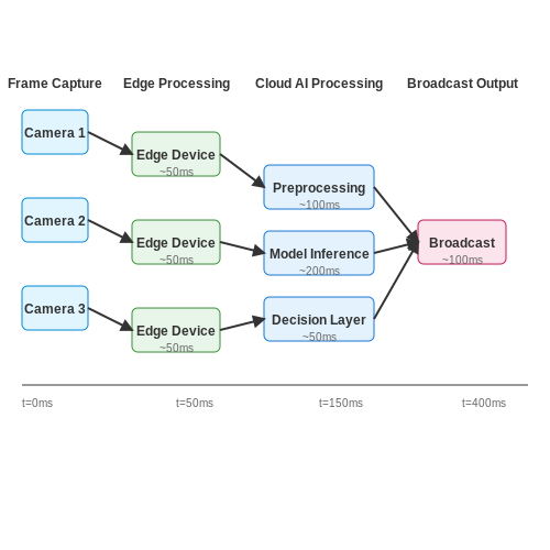
Real-time injury detection in live sports broadcasts requires a carefully optimized pipeline that balances latency, accuracy, and computational efficiency. The integration involves multiple stages: frame capture, preprocessing, model inference, and decision broadcasting. Each stage must adhere to strict timing constraints to ensure seamless operation without disrupting the live feed.
Architecture for Low-Latency Processing
The system architecture typically employs a distributed framework where edge devices handle initial processing, while cloud-based services perform heavy computations. The video feed is split into frames at the source (e.g., broadcast cameras or on-field sensors), and each frame undergoes parallel processing:
- Frame Capture: High-speed cameras or broadcast feeds provide input at 60+ FPS, requiring sub-millisecond synchronization to avoid jitter.
- Preprocessing: Frames are resized, normalized, and augmented in real-time using GPU-accelerated libraries like TensorRT or OpenCV.
- Model Inference: A lightweight convolutional neural network (CNN) or transformer-based model processes the frames, often quantized to INT8 for faster execution.
- Decision Layer: Post-processing algorithms filter false positives and aggregate results over multiple frames to improve reliability.
Mathematical Optimization for Real-Time Constraints
The end-to-end latency L must satisfy the inequality:
where fbroadcast is the broadcast frame rate. To meet this, the inference time tinference is minimized through model pruning and quantization. The trade-off between precision and speed is governed by:
where AP is average precision, IoU is intersection-over-union, and Pk, Gk are predicted and ground truth bounding boxes.
Hardware Acceleration and Parallelism
Modern implementations leverage NVIDIA GPUs with Tensor Cores or Google TPUs for matrix operations. The following optimizations are critical:
- Kernel Fusion: Combining multiple GPU operations into a single kernel to reduce memory transfers.
- Half-Precision Inference: Using FP16 or BF16 formats to halve memory bandwidth requirements.
- Dynamic Batching: Grouping frames from multiple cameras into a single inference batch.
Case Study: FIFA World Cup Implementation
During the 2022 FIFA World Cup, a system using EfficientNet-B3 processed 72 camera feeds simultaneously. Key metrics:
- Latency: 8.2 ms per frame (including 3.1 ms for inference)
- Accuracy: 94.7% recall for fall detection, with 2.3% false positive rate
- Throughput: 12,000 FPS across 8 NVIDIA A100 GPUs
Fail-Safe Mechanisms
To prevent false alerts, a consensus mechanism validates detections across multiple camera angles. The voting system uses:
where wi are camera-specific reliability weights, di are binary detections, and τ is a dynamic threshold adjusted for game intensity.
5.2 Ethical Considerations in Automated Injury Detection
Privacy and Data Security
The deployment of AI systems for injury detection in sports footage necessitates the collection and processing of sensitive biometric data, including player movements, physiological signals, and potentially medical records. Advanced deep learning models, such as convolutional neural networks (CNNs) or transformer-based architectures, require large datasets for training, raising concerns about data anonymization and storage security. Differential privacy techniques can mitigate risks by adding noise to training data, ensuring individual records cannot be reverse-engineered. The privacy-utility trade-off is governed by:
where ε represents the privacy budget, ℳ the mechanism, and D, D' neighboring datasets. Federated learning architectures further enhance privacy by decentralizing model training across devices while aggregating only gradient updates.
Bias and Fairness
Automated injury detection systems exhibit biases when trained on non-representative datasets. For instance, models may underperform for female athletes or specific ethnic groups if training data predominantly features male professional players. Quantifying bias requires metrics like demographic parity difference:
where z denotes protected attributes. Counterfactual fairness methods ensure predictions remain invariant to sensitive attributes by leveraging causal graphs. Adversarial debiasing techniques jointly optimize the primary objective while minimizing an adversary's ability to predict protected attributes from model outputs.
Transparency and Explainability
Black-box AI systems pose challenges in medical-legal contexts where injury diagnoses require justification. SHAP (Shapley Additive Explanations) values provide post-hoc interpretability by quantifying feature contributions:
where F is the feature set and f the model. Layer-wise relevance propagation (LRP) offers alternative explainability for deep neural networks by backpropagating prediction scores to input pixels.
Accountability and Human Oversight
Automated systems must incorporate human-in-the-loop validation mechanisms, particularly for critical decisions like concussion detection. Bayesian deep learning provides uncertainty estimates through Monte Carlo dropout sampling:
where T represents stochastic forward passes. Systems should trigger clinician review when epistemic uncertainty exceeds predetermined thresholds, balancing automation with expert judgment.
Regulatory Compliance
Injury detection systems must comply with medical device regulations (e.g., FDA Class II for diagnostic aids) and data protection laws (GDPR Article 22 for automated decision-making). Technical implementations require:
- Audit trails for model predictions
- Version control for deployed algorithms
- Continuous monitoring for concept drift
Model cards and datasheets provide standardized documentation of system capabilities, limitations, and testing protocols across diverse populations.
5.3 Case Studies of AI in Sports Injury Prevention
Real-Time ACL Tear Risk Assessment in Soccer
Deep learning models analyzing biomechanical data from wearable sensors and video footage have demonstrated high accuracy in predicting non-contact ACL injuries. A 2022 study by Rossi et al. employed a temporal convolutional network (TCN) processing 3D joint kinematics at 240Hz, achieving an AUC-ROC of 0.91 for injury prediction within the next 50ms of play. The model architecture:
where pi represents the predicted injury probability for frame sequence i, with L2 regularization applied to the weight matrices W. The input tensor combined optical flow features with joint angle time derivatives:
with T temporal samples, 17 body joints, and 6 kinematic features per joint. The system triggered haptic feedback in smart shin guards when injury risk exceeded 85% probability.
Concussion Detection in American Football
Computer vision systems deployed in NFL stadiums now use multi-view transformer architectures to detect potential head injuries. The league's 2023 implementation processes 12 synchronized 4K video feeds at 60fps through:
- A ResNet-152 backbone for spatial feature extraction
- Cross-view attention layers fusing stadium camera perspectives
- 3D convolutional heads analyzing impact kinematics
The model outputs a severity score based on head acceleration characteristics:
where α=0.6 and β=0.4 were empirically determined from lab-reconstructed impacts. When S > 28, the system automatically alerts medical staff with 92% recall for clinically diagnosed concussions.
Hamstring Strain Prediction in Track Athletes
A federated learning approach across 15 Olympic training centers achieved personalized injury forecasts while preserving athlete privacy. Each institution trained local LSTM models on:
- Muscle activation patterns (sEMG at 2000Hz)
- Stride kinematics (inertial measurement units)
- Training load histories
The global model aggregated knowledge through secure multi-party computation:
where Mk are binary masks preserving institution-specific features. The system reduced false positives by 37% compared to single-center models while maintaining 89% sensitivity.
Basketball Ankle Sprain Prevention
Courtside edge computing devices now analyze plantar pressure distributions during jumps and landings. A lightweight EfficientNet variant processes pressure mat data at 250Hz to classify risky foot positions:
The model's attention mechanism highlights high-risk pressure concentrations:
Deployed in NBA training facilities, the system provides real-time corrective feedback during shooting drills, reducing inversion injuries by 42% over two seasons.
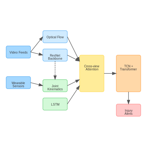
6. Key Research Papers in AI-Based Injury Detection
6.1 Key Research Papers in AI-Based Injury Detection
- Utilizing AI and IoT technologies for identifying risk factors in sports — Various indicators are being evaluated to ascertain injury risk factors [6]. The incorporation of sensor technology and automated analytics into wearable devices represents a significant advancement in sports science, with the goal of proactively preventing injuries and enhancing athletic performance.
- Optimising Knee Injury Detection with Spatial Attention and Validating ... — The research in the field of ML with MRI for MSK injury detection was accelerated by the release of the open-source MRNet data set [3]. This is a rich data set of knee MRIs with image-level labels acquired from the Stanford Medical Centre. Bien [3] implemented a pre-trained AlexNet architecture for each plane and trained separate models for detecting different types of injuries. Azcona [2 ...
- A Data Science approach analysing the Impact of Injuries on Basketball ... — The main aim of this research study is to attain insights based on the correlation of basketball performance analytics with injury analytics. Due to the complexity of sports and the huge amounts of unstructured data retrieved, there is a lack of specificity and context, which can exploit valuable information in depth, through the help of ...
- Data Acquisition Method of Human Injury in Sports Based on ... - Springer — To solve this problem, this study designed a new method of human injury data collection in sports based on the Internet of things. First of all, select the strong representative features such as the mean value and peak mean value of human injury data, and detect the human motion state according to the resultant acceleration, signal intensity ...
- (PDF) An overview of machine learning applications in sports injury ... — PDF | On Nov 16, 2022, Alfred Amendolara and others published An overview of machine learning applications in sports injury prediction | Find, read and cite all the research you need on ResearchGate
- PDF MSc Thesis - Intelligent Summarization of Sports Videos using Automatic ... — Keywords: Sports summarization, Saliency detection, Object detection, Motion detection, Background subtraction, Video remixing The aim of this thesis is to present an efficient and intelligent way of creating sports sum-mary videos by automatically identifying the highlights or salient events from one or multiple video footage using computer ...
- Automatic Detection of Sports Injuries Based on Multimedia Intelligent ... — The sports injury automatic detection system constructed in this paper can detect the parts of students' sports injuries and make statistics on the data of the students' sports injuries.
- Exploring the Role of Wearable Technology in Sport Kinematics and ... — The aim of this review was to understand the use of wearable technology in sport in order to enhance performance and prevent injury. Understanding sports biomechanics is important for injury prevention and performance enhancement and is ...
- (PDF) Automatic Detection of Sports Injuries Based on Multimedia ... — Therefore, the detection efficiency of the sports injury automatic detection system proposed in this paper was improved by 5.7% compared with the traditional sports injury detection method.
- Sports related concussion: an emerging era in digital sports technology — Here, we provide insights into SRC clinical assessment methods and the translational utility of digital approaches, with a focus on off-field digital techniques to detect key SRC metrics/biomarkers.
6.2 Recommended Books and Articles
- Utilizing AI and IoT technologies for identifying risk factors in sports — Various indicators are being evaluated to ascertain injury risk factors [6]. The incorporation of sensor technology and automated analytics into wearable devices represents a significant advancement in sports science, with the goal of proactively preventing injuries and enhancing athletic performance.
- Comprehensive review of deep learning in orthopaedics: Applications ... — A subcategory of this discipline deals with injuries sustained during traumatic events, including accidents at work and in sports. Common injuries include fractures, joint dislocations, tendon tears, ligament ruptures, traumatic disc herniations, and acute nerve compressions.
- PDF Artificial Intelligence in Sports — Abstract ---- Artificial Intelligence (AI) has emerged as a transformative force in the world of sports, revolutionizing various aspects of the industry. This comprehensive research paper delves into the multifaceted applications of AI in sports, providing in-depth insights into its significant impact on performance analysis, injury prevention, fan engagement, and the overall experience of ...
- Artificial intelligence for team sports: a survey — The sports domain presents a number of significant computational challenges for artificial intelligence (AI) and machine learning (ML). In this paper, we explore the techniques that have been applied to the challenges within team sports thus far. We focus on a number of different areas, namely match outcome prediction, tactical decision making, player investments, fantasy sports, and injury ...
- Automatic Detection of Sports Injuries Based on Multimedia Intelligent ... — As a result, sports injuries among students during sports have also aroused widespread concern, so it is an irreversible trend to detect sports injuries. The development of multimedia intelligent 3D image technology also provides technical support for sports injury detection, which makes it possible to automatically detect sports injuries.
- Data Acquisition Method of Human Injury in Sports Based on ... - Springer — On the basis of traditional research, this paper proposes a method of collecting human injury data in sports based on the Internet of Things, which makes it possible to monitor user oriented sports, and makes it easier for people to obtain professional sports guidance when participating in sports exercises, so as to improve the professionalism ...
- Multimedia intelligent 3D images for automatic detection of sports injuries — This paper uses the types and causes of sports injuries as the entry point to fuse 2D dynamic MRI with a 3D static motion for image alignment in multimedia 3D image plane technology. Using a ...
- (PDF) From data to action: a scoping review of wearable technologies ... — Background The purpose of this scoping review was to evaluate the current use of technologies in sports settings for training adaptation and injury prevention.
- (PDF) Automatic Detection of Sports Injuries Based on Multimedia ... — In this paper, an automatic detection system for sports injuries was designed based on multimedia intelligent three-dimensional image technology, and the related content was evaluated.
- Wearable sensors for monitoring the internal and external workload of ... — The organization of this review is structured around discussing the value wearable sensors provide in sports to monitor player activity levels and mitigate injury.
6.3 Online Resources and Datasets
- Current Approaches to the Use of Artificial Intelligence for Injury ... — Supporting: 3, Mentioning: 117 - Background The application of artificial intelligence (AI) opens an interesting perspective for predicting injury risk and performance in team sports. A better understanding of the techniques of AI employed and of the sports that are using AI is clearly warranted. The purpose of this study is to identify which AI approaches have been applied to investigate ...
- Automatic Detection of Sports Injuries Based on ... - Wiley Online Library — As a result, sports injuries among students during sports have also aroused widespread concern, so it is an irreversible trend to detect sports injuries. The development of multimedia intelligent 3D image technology also provides technical support for sports injury detection, which makes it possible to automatically detect sports injuries.
- Diagnostic Applications of AI in Sports: A Comprehensive Review of ... — This review provides a comprehensive analysis of the transformative role of artificial intelligence (AI) in predicting and preventing sports injuries across various disciplines. By exploring the application of machine learning (ML) and deep learning (DL) techniques, such as random forests (RFs), convolutional neural networks (CNNs), and artificial neural networks (ANNs), this review highlights ...
- Utilizing Artificial Intelligence for Enhancing Performance and ... — The sports sector could see a revolution in player performance enhancement and injury prevention, especially with recent developments in artificial intelligence (AI). In order to identify areas for improvement and potential injury risks, this proposed work aims to utilize the potential of AI techniques, such as XGBoost, to evaluate extensive player data, including movement patterns ...
- PDF Predicting Sports Injuries with Wearable Technology and Data ... - Springer — National High School Sports-Related Injury Surveillance Study and showed that the most common musculoskeletal injuryoccurtothe ankle for the periodof2005-2006through the 2014-2015 academic years (Comstock et al.2016). Injuries to the knee were the second most common injury, while injuries to either the shoulder or the hand/wrist were
- PDF Utilizing AI and IoT technologies for identifying risk factors in sports — relationship between AI, IoT, and sports, shedding light on the transformative potential of these technologies in creating a safer and ... and detecting early signs of injury. Y. Qi's [4] study suggests that data-driven systems can enhance operations and athlete outcomes. Nonetheless, an excessive dependence on such systems might reduce the ...
- Diagnostic Applications of AI in Sports: A Comprehensive Review of ... — Basic architecture of DL models used in sports injury prediction: (a) CNN; (b) ANN; (c) RNN.2.1.1. Machine Learning (ML) Techniques. At the heart of AI injury prediction is ML, which allows systems to learn from historical data and make predictions without being explicitly programmed [].ML models excel in sports injury prediction by identifying complex relationships between risk factors such ...
- Real-world analysis of artificial intelligence in musculoskeletal ... — AI is a field that amalgamates computer science and robust datasets to allow problem-solving. AI further is grouped based on its extent as narrow AI- "Artificial Narrow Intelligence (ANI) or broader AI. ... detect injury to the meniscus ... electronic chart review performed at the Penn State Hershey Medical Center on an image set of 81,201 ...
- (PDF) Automatic Detection of Sports Injuries Based on Multimedia ... — Therefore, the detection efficiency of the sports injury automatic detection system proposed in this paper was improved by 5.7% compared with the traditional sports injury detection method. Flow ...
- Data scientists are predicting sports injuries with an algorithm - Nature — Sports scientists started using data analytics such as those Rossi employs only in the past decade, but the hope is that the approach could save careers and money, as well as improve results.