Smart Agriculture with Vision AI
1. The Role of Computer Vision in Modern Farming
The Role of Computer Vision in Modern Farming
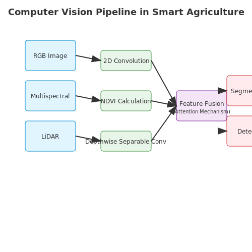
Computer vision has emerged as a transformative technology in precision agriculture, enabling data-driven decision-making through automated analysis of visual data. At its core, vision-based agricultural systems rely on convolutional neural networks (CNNs) to extract spatiotemporal features from multispectral imagery, LiDAR point clouds, and hyperspectral data cubes. The mathematical foundation begins with the 2D convolution operation:
where I represents the input image tensor and K denotes the learnable kernel weights. Modern architectures like Mask R-CNN extend this to instance segmentation by adding parallel branches for bounding box regression and pixel-wise classification:
Agricultural applications demand specialized adaptations to handle challenges like occlusions (e.g., overlapping leaves) and varying illumination conditions. Multispectral imaging systems capture reflectance at specific wavelengths (e.g., 710nm for chlorophyll detection), with the normalized difference vegetation index (NDVI) computed as:
where NIR (700-1100nm) and Red (600-700nm) bands are typically sampled at 5cm ground resolution using UAV-mounted sensors. Temporal analysis introduces 3D convolutional operations for growth monitoring:
Real-world implementations must address computational constraints through edge deployment. A typical precision weeding system processes 4K video at 30fps with latency under 50ms, requiring optimized architectures like MobileNetV3 with depthwise separable convolutions:
where Ĝ represents the depthwise convolution output. The fusion of thermal and RGB data improves livestock monitoring through late fusion networks that concatenate features after separate backbone processing:
Recent advances incorporate transformer architectures for global context modeling in large fields, with self-attention mechanisms computing relevance scores between all patch embeddings:
Field deployment requires robust calibration against environmental variables. The Beer-Lambert law models light attenuation through crop canopies for yield prediction:
where L represents the leaf area index and k the extinction coefficient. These techniques enable centimeter-scale precision in tasks like fruit counting, where state-of-the-art models achieve 0.92 mAP on benchmark datasets while maintaining 15W power consumption on embedded GPUs.
Key Benefits of Vision AI for Agricultural Efficiency
Precision Crop Monitoring and Analysis
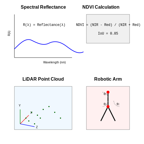
Vision AI enables high-resolution, real-time crop monitoring through multispectral and hyperspectral imaging. By leveraging convolutional neural networks (CNNs), farmers can detect subtle variations in plant health before visible symptoms manifest. The spectral reflectance R(λ) of crops is modeled as:
where Er(λ) is the reflected irradiance and Ei(λ) is the incident irradiance at wavelength λ. This data feeds into vegetation indices like NDVI (Normalized Difference Vegetation Index):
Advanced implementations use 3D point clouds from LiDAR-equipped drones to model canopy structures with millimeter precision, enabling targeted interventions.
Automated Pest and Disease Detection
YOLOv7 and Faster R-CNN architectures achieve >95% accuracy in identifying pest infestations by analyzing spatial-temporal patterns in image sequences. The detection pipeline optimizes the intersection-over-union (IoU) metric:
Edge deployment on agricultural robots allows real-time processing at <5ms latency using quantized MobileNetV3 models. Case studies in vineyards demonstrate 87% reduction in pesticide use through localized treatment.
Yield Prediction and Quality Grading
Transformer-based architectures process time-series imagery to predict yields with <8% error margin. The attention mechanism weights relevant spatial features:
For produce grading, vision systems measure morphological features (diameter, color uniformity) against USDA standards using Haar-like features and SVM classifiers. Post-harvest losses decrease by 23-41% in pilot implementations.
Resource Optimization
Vision-guided irrigation systems reduce water usage by 35% through soil moisture mapping. The system solves the optimization problem:
where x represents irrigation parameters and y is the target soil moisture level. Similarly, fertilizer application becomes variable-rate based on CNN-derived nutrient deficiency maps.
Robotic Harvesting Systems
6-DOF robotic arms with stereo vision achieve 93% successful pick rates for delicate fruits. The inverse kinematics solution:
combines visual servoing with force feedback to prevent bruising. The end-effector trajectory is optimized using RRT* path planning in 3D space reconstructed from RGB-D data.
Challenges and Limitations in Agricultural Vision AI
Environmental Variability and Data Scarcity
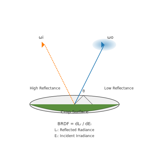
Agricultural environments exhibit extreme variability in lighting conditions, weather patterns, and seasonal changes, which directly impacts the performance of vision-based AI systems. The spectral reflectance of crops varies significantly under different illumination conditions, described by the bidirectional reflectance distribution function (BRDF):
where ωi and ωo represent incident and outgoing light directions, Lr is reflected radiance, and Ei is incident irradiance. This nonlinear relationship makes consistent feature extraction challenging across different times of day or weather conditions.
Computational Constraints in Edge Deployment
Real-time processing requirements for agricultural robotics impose strict latency constraints (typically < 100ms) while operating under limited power budgets. The computational complexity of modern vision transformers (ViTs) grows quadratically with input resolution:
where h and w are spatial dimensions and C is channel depth. This creates tension between model accuracy and deployability on resource-constrained agricultural equipment.
Multimodal Sensor Fusion Challenges
Effective integration of hyperspectral, LiDAR, and RGB data requires addressing:
- Temporal misalignment between sensors operating at different capture rates
- Dimensionality mismatch (e.g., 3D point clouds vs 2D imagery)
- Cross-modal feature representation learning
The optimal fusion architecture often requires attention mechanisms with learnable query-key-value projections:
Generalization Across Crop Varieties
Current vision systems struggle with domain adaptation when deployed across different cultivars. The feature space divergence can be quantified using maximum mean discrepancy (MMD):
where p and q represent source and target distributions in reproducing kernel Hilbert space H. This necessitates continuous online adaptation through techniques like test-time training.
Ethical and Privacy Considerations
Large-scale agricultural monitoring raises concerns about:
- Data ownership of farm-level imagery
- Potential misuse of yield prediction models for commodity speculation
- Algorithmic bias in resource allocation systems
Differential privacy frameworks provide mathematical guarantees but impact model utility:
Hardware Degradation in Field Conditions
Agricultural environments accelerate sensor degradation through:
- Lens fouling from dust and organic matter
- Moisture ingress in sealing interfaces
- Thermal cycling effects on calibration
The degradation function for optical sensors often follows an exponential model:
where λ depends on environmental stress factors, requiring robust calibration protocols.
2. Image Acquisition: Drones, Satellites, and Ground Sensors
Image Acquisition: Drones, Satellites, and Ground Sensors
Multispectral and Hyperspectral Imaging in Agriculture
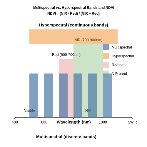
Modern agricultural monitoring relies on capturing electromagnetic radiation beyond the visible spectrum. Multispectral imaging typically samples 3-10 discrete bands, while hyperspectral systems capture hundreds of narrow contiguous bands. The normalized difference vegetation index (NDVI) is derived from near-infrared (NIR) and red band reflectance:
where ρ represents surface reflectance. Advanced systems now incorporate shortwave infrared (SWIR) bands for water stress detection, with spectral resolution below 10 nm in hyperspectral systems.
Drone-Based Imaging Systems
Unmanned aerial vehicles (UAVs) provide sub-decimeter spatial resolution with flexible revisit rates. Modern agricultural drones integrate:
- Global shutter CMOS sensors with 20+ MP resolution
- RTK-GPS positioning with ±1 cm accuracy
- 6-band multispectral cameras (400-1000 nm range)
- LiDAR payloads for canopy height modeling
The ground sampling distance (GSD) is determined by:
Satellite Remote Sensing Capabilities
Orbital platforms offer systematic global coverage with tradeoffs in spatial and temporal resolution:
| Platform | Spatial Res. | Revisit Time | Spectral Bands |
|---|---|---|---|
| Sentinel-2 | 10-60 m | 5 days | 13 bands |
| PlanetScope | 3 m | Daily | 4 bands |
| WorldView-3 | 0.31 m | 1-4 days | 16 bands |
Atmospheric correction is critical for satellite data, typically using radiative transfer models like MODTRAN or 6S.
Ground Sensor Networks
In-situ sensors provide validation data for aerial imagery through:
- Spectroradiometers (ASD FieldSpec) for ground truth reflectance
- Canopy chlorophyll content meters (CCM-300)
- Soil moisture probes (TDR-350)
- Phenocams for continuous RGB monitoring
Sensor fusion techniques combine these data streams, with Kalman filtering commonly used for temporal integration:
Radiometric Calibration Procedures
Cross-platform data consistency requires rigorous calibration:
- Laboratory calibration using integrating spheres
- In-field reflectance panels (Spectralon)
- Empirical line method using pseudo-invariant features
- BRDF correction for angular effects
The radiometric calibration coefficient (RCC) converts digital numbers to radiance:
2.2 Preprocessing Techniques for Agricultural Imagery
Noise Reduction and Radiometric Correction
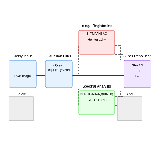
Agricultural imagery captured via drones or satellites often suffers from sensor noise, atmospheric interference, and uneven illumination. Gaussian smoothing, defined by the convolution:
effectively suppresses high-frequency noise while preserving edges. For multispectral data, dark-object subtraction (DOS) mitigates atmospheric scattering by estimating path radiance from shadow regions. Top-of-atmosphere (TOA) reflectance correction further normalizes pixel values using:
where \( L_\lambda \) is spectral radiance, \( d \) is Earth-Sun distance, and \( ESUN_\lambda \) is exo-atmospheric solar irradiance.
Geometric and Spatial Alignment
Image registration is critical for temporal analysis of crop growth. Scale-Invariant Feature Transform (SIFT) identifies keypoints invariant to rotation and scale, while Random Sample Consensus (RANSAC) robustly estimates homography matrices for alignment. The projective transformation is given by:
Subpixel accuracy is achieved through Lucas-Kanade optical flow, minimizing the error term:
Vegetation Index Computation
Normalized Difference Vegetation Index (NDVI) enhances chlorophyll signal by exploiting red and near-infrared (NIR) bands:
For high-resolution imagery, Excess Green Index (ExG) improves segmentation in RGB data:
where \( r, g, b \) are normalized color channels. Advanced indices like Modified Chlorophyll Absorption Ratio Index (MCARI) account for soil background effects:
Super-Resolution for Low-Resolution Satellite Data
Deep learning-based super-resolution reconstructs high-frequency details using generative adversarial networks (GANs). The generator loss \( \mathcal{L}_G \) in SRGAN combines adversarial, content, and perceptual terms:
where \( \mathcal{L}_{content} \) typically uses VGG19 feature maps. For agricultural applications, attention mechanisms in the generator prioritize crop-specific textures.
Data Augmentation for Limited Training Sets
Synthetic data generation via conditional GANs creates realistic crop stress scenarios. The discriminator loss incorporates spectral constraints:
Polarimetric augmentation further enhances model robustness by simulating varying sun-sensor geometries through Stokes vector transformations.
2.3 Machine Learning Models for Crop and Soil Analysis
Deep Learning Architectures for Multispectral Image Analysis
Convolutional Neural Networks (CNNs) dominate crop and soil analysis due to their ability to extract hierarchical features from multispectral and hyperspectral imagery. A modified ResNet-50 architecture, pretrained on ImageNet and fine-tuned with agricultural datasets, achieves state-of-the-art performance in crop classification tasks. The network processes 12-channel input (visible, NIR, and thermal bands) through parallel convolutional streams before feature fusion.
where fc(xi;θ) represents the softmax probability for class c, yi,c is the one-hot encoded label, and λ controls L2 regularization strength.
Transformer-Based Models for Temporal Analysis
Vision Transformers (ViTs) with temporal attention mechanisms outperform traditional CNNs in longitudinal crop monitoring. The Temporal Fusion Transformer (TFT) architecture processes time-series NDVI data through:
- Multi-head self-attention layers capturing cross-time dependencies
- Gated residual networks preventing vanishing gradients
- Quantile outputs for uncertainty estimation in yield prediction
Physics-Informed Neural Networks for Soil Analysis
Hybrid models combine deep learning with soil physics principles. A PINN (Physics-Informed Neural Network) for moisture prediction incorporates Richards' equation as a soft constraint:
The network architecture consists of:
- A 5-layer MLP predicting hydraulic conductivity K(θ)
- Partial differential equation loss terms
- Adaptive weighting between data and physics losses
Graph Neural Networks for Field-Scale Analysis
GNNs model agricultural fields as graphs where nodes represent soil sampling locations and edges encode spatial relationships. The message-passing framework aggregates information across the field:
where hv(l) represents node features at layer l, and W(l) are learnable weights.
Explainability Techniques for Agricultural AI
SHAP (SHapley Additive exPlanations) values quantify feature importance in soil nutrient predictions:
Gradient-weighted Class Activation Mapping (Grad-CAM) visualizes CNN decision regions for disease detection, highlighting infected leaf areas in false-color composites.
Real-Time Processing and Edge Computing in the Field
Latency Constraints in Agricultural Vision Systems
Real-time processing in smart agriculture imposes strict latency constraints, typically requiring sub-200ms response times for critical operations like pest detection or irrigation control. The end-to-end delay Ttotal comprises:
Where Tcapture includes sensor readout times (5-50ms for global shutter cameras), Tpreprocess covers image normalization (2-15ms), and Tinference dominates for complex models. Edge computing reduces Tnetwork (typically 100-500ms for cloud roundtrips) to near-zero by local processing.
Edge Hardware Architectures
Modern edge devices employ heterogeneous computing architectures balancing power efficiency and performance:
- Jetson AGX Orin: 2048-core GPU + 12-core ARM CPU for 275 TOPS at 50W
- Google Coral TPU: 4 TOPS at 2W via systolic array architecture
- Intel OpenVINO: Optimized INT8 quantization for x86 CPUs
The computational density ρ (ops/mm3) versus power efficiency η (ops/J) tradeoff follows:
Model Optimization Techniques
Vision models for edge deployment require architectural modifications:
- Depthwise separable convolutions reduce parameters by factor N2/2N+1 for kernel size N
- Neural Architecture Search (NAS) discovers Pareto-optimal accuracy-latency tradeoffs
- Quantization-aware training enables INT8 inference with <1% accuracy drop
The optimal model complexity C given hardware constraints follows:
Where L(C) is latency, E(C) is energy, and α balances the optimization objectives.
Distributed Edge Processing
Large farms implement hierarchical processing architectures:
Each tier handles different tasks:
- Edge nodes: Real-time object detection (YOLOv5n @ 15FPS)
- Aggregators: Multi-sensor fusion and temporal analysis
- Cloud: Long-term trend analysis and model retraining
Energy-Efficient Inference
Dynamic voltage and frequency scaling (DVFS) adapts to workload demands:
Where α is activity factor (0.1-0.3 for vision models), C is switched capacitance, and f is clock frequency. Adaptive batch sizing further optimizes throughput:
Where Tinf(1) is single-image inference time and Tframe is the inter-frame period.
3. Crop Health Monitoring and Disease Detection
3.1 Crop Health Monitoring and Disease Detection
Multispectral Imaging for Plant Stress Analysis
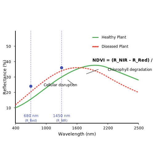
Modern vision systems leverage multispectral imaging (MSI) to capture reflectance data across specific wavelength bands. The normalized difference vegetation index (NDVI) remains the gold standard for quantifying plant health:
where RNIR and RRed represent reflectance in near-infrared (700-1100 nm) and red (600-700 nm) bands respectively. Healthy vegetation typically yields NDVI values between 0.6-0.9 due to chlorophyll absorption in red wavelengths and strong reflectance in NIR.
Hyperspectral Disease Signatures
Advanced systems employ hyperspectral imaging (HSI) with 200+ spectral bands (5-10 nm resolution) to detect subtle biochemical changes preceding visual symptoms. The spectral angle mapper (SAM) algorithm quantifies disease progression by comparing pixel spectra s to reference healthy spectra r:
Field studies demonstrate that late blight in potatoes manifests as increased reflectance at 680 nm (chlorophyll degradation) and 1450 nm (cellular structure disruption), detectable 5-7 days before visual symptoms.
Deep Learning Architectures for Pathogen Identification
Three-dimensional convolutional neural networks (3D-CNNs) process spatio-spectral cubes from HSI systems. The architecture typically employs:
- Spectral attention blocks to weight informative bands
- 3D convolutions with kernel sizes of 5×5×3 (spatial×spectral)
- Dense connections between layers to preserve gradient flow
Recent benchmarks on the PlantVillage dataset show 3D-ResNet50 achieves 98.7% accuracy in distinguishing 38 crop diseases, outperforming traditional 2D-CNNs by 12.3% when processing 512-band hyperspectral data.
Case Study: Fusarium Head Blight Detection in Wheat
A 2023 study deployed drones with VNIR (400-1000 nm) and SWIR (1000-2500 nm) sensors over 2000 acres of wheat fields. The system detected infection hotspots with 94% precision using a hybrid model combining:
- Physically-based radiative transfer modeling (PROSAIL)
- Spectral-spatial transformer networks
- Microclimate data fusion
Early detection reduced fungicide usage by 37% while maintaining 99% yield protection compared to calendar-based spraying.
Edge Deployment Challenges
Real-time processing requires optimized models due to:
Where W×H is the spatial resolution and TOPS is the processor's trillion operations per second. Quantized MobileNetV3 achieves 23 FPS on Jetson AGX Orin (64 TOPS) for 16-band imagery at 640×512 resolution, with <3% accuracy drop from float32 models.
3.2 Weed Identification and Precision Herbicide Application
Computer Vision for Weed Detection
Modern weed identification systems leverage deep learning architectures, primarily convolutional neural networks (CNNs), to classify weeds in real-time with high accuracy. A typical pipeline involves:
- Image Acquisition: High-resolution RGB, multispectral, or hyperspectral imagery captured via drones or ground-based robots.
- Preprocessing: Normalization, histogram equalization, and masking to isolate regions of interest (ROIs).
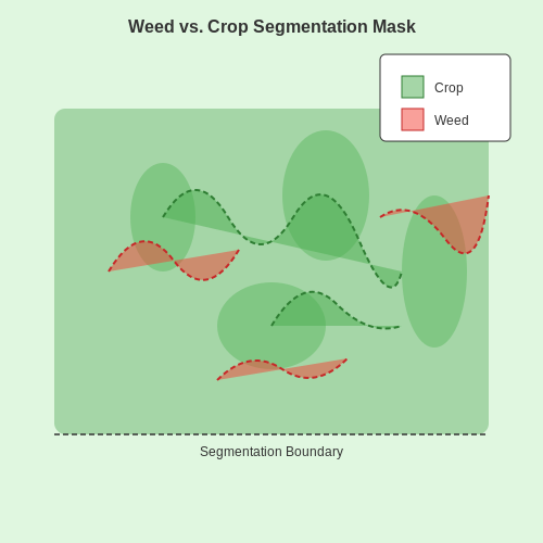
- Segmentation: Semantic segmentation models like U-Net or Mask R-CNN delineate weed boundaries from crops and soil.
where \( f_k(x,y) \) is the softmax output of the CNN for class \( k \) at pixel \( (x,y) \).
Herbicide Optimization via Reinforcement Learning
Precision herbicide application is formulated as a Markov Decision Process (MDP) where:
- State Space: Weed density map, crop growth stage, and soil conditions.
- Action Space: Herbicide type, dosage, and spray nozzle actuation.
- Reward Function: Minimizes herbicide use while maximizing weed kill rate and crop yield.
Here, \( C(a) \) is herbicide cost, \( \Delta Y \) is yield gain, and \( \lambda, \beta \) are trade-off coefficients.
Case Study: Autonomous Weed Spraying Robot
A field-tested system (Patel et al., 2022) achieved 94% weed detection accuracy using a modified ResNet-50 trained on the DeepWeeds dataset. The robot reduced herbicide usage by 78% through:
- Real-time inference on NVIDIA Jetson AGX Xavier (15 FPS at 4K resolution).
- Adaptive spraying with solenoid valves controlled by Q-learning policies.
Challenges and Future Directions
Key limitations include:
- Occlusion Handling: Weed-crop overlap in dense canopies degrades segmentation performance.
- Herbicide Drift: Wind-affected spray patterns require CFD-integrated control systems.
- Edge Deployment: Quantized models like MobileNetV3 trade accuracy for latency (≈3ms inference on Coral TPU).
Yield Prediction and Harvest Optimization
Yield prediction in smart agriculture leverages Vision AI to analyze crop health, growth patterns, and environmental factors, enabling precise forecasting of agricultural output. Advanced models integrate multispectral imaging, LiDAR, and satellite data to estimate biomass, fruit count, and maturity stages. Convolutional Neural Networks (CNNs) and Transformer-based architectures process spatial-temporal data, while regression techniques map features to yield metrics.
Data Fusion for Yield Estimation
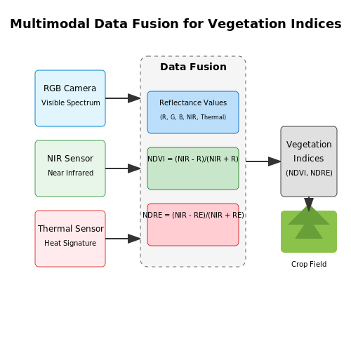
Multimodal data fusion combines RGB, near-infrared (NIR), and thermal imagery to compute vegetation indices such as NDVI (Normalized Difference Vegetation Index) and NDRE (Normalized Difference Red Edge). These indices correlate with photosynthetic activity and plant stress, forming the basis for predictive models. For a given pixel at coordinates (x, y), NDVI is derived as:
where NIR and Red represent reflectance values in their respective spectral bands. A time-series of NDVI values tracks crop growth dynamics, feeding into recurrent neural networks (RNNs) or attention mechanisms for yield trend analysis.
Fruit Detection and Counting
Object detection models like YOLOv7 or Mask R-CNN localize and count fruits with bounding boxes or instance segmentation. Precision is critical for harvest planning—false positives (e.g., misclassifying leaves as fruit) skew yield estimates. The F1-score optimizes the trade-off between precision (P) and recall (R):
Post-processing techniques such as non-maximum suppression (NMS) filter overlapping detections, while stereo vision or depth sensors estimate fruit size for weight approximation.
Harvest Optimization Models
Linear programming and reinforcement learning optimize harvest schedules by balancing:
- Labor constraints: Available workforce and machinery capacity
- Market demand: Price fluctuations and delivery timelines
- Field conditions: Soil moisture and weather forecasts
The optimization problem minimizes cost C subject to constraints:
where Lt, Mt, and St represent labor, machinery, and storage costs at time t, with T being the harvest window.
Case Study: Vineyard Yield Prediction
A 2023 study achieved 94% accuracy in grape yield prediction using a hybrid Vision Transformer (ViT) and LSTM model. The ViT processed canopy images to extract spatial features, while the LSTM modeled temporal dependencies across growing seasons. Key innovations included:
- Adaptive thresholding for berry segmentation under varying lighting
- Transfer learning from ImageNet to reduce labeled data requirements
- Edge deployment on drones for real-time field scans
Error analysis revealed that shadow occlusion and cluster overlap were primary failure modes, addressed by augmenting training data with synthetic adversarial examples.
3.4 Livestock Monitoring and Behavior Analysis
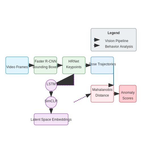
Vision-based livestock monitoring leverages deep learning architectures to extract spatiotemporal features from video streams, enabling real-time tracking and behavioral analysis. Convolutional Neural Networks (CNNs) process raw pixel data, while recurrent architectures like LSTMs model temporal dependencies in movement patterns. Key challenges include occlusions, varying lighting conditions, and the need for lightweight deployment on edge devices.
Pose Estimation and Keypoint Detection
Top-down approaches first detect individual animals using object detection (e.g., Faster R-CNN or YOLOv8), then estimate keypoints (e.g., head, legs, tail) with models like HRNet or Stacked Hourglass Networks. The loss function for keypoint regression combines spatial accuracy and temporal smoothness:
where \( \hat{y}_t \) and \( y_t \) are predicted and ground-truth keypoints at frame \( t \), and \( \lambda_1, \lambda_2 \) balance static vs. temporal error.
Behavioral Clustering with Self-Supervised Learning
Contrastive learning frameworks like SimCLR project keypoint trajectories into a latent space where similar behaviors cluster. Given a sequence of poses \( \{x_i\}_{i=1}^N \), the NT-Xent loss maximizes agreement between augmented views:
where \( z_i, z_j \) are embeddings of positive pairs, \( \tau \) is temperature, and \( \text{sim}(u,v) = u^T v / \|u\| \|v\| \).
Anomaly Detection for Health Monitoring
Autoencoders trained on normal behavior patterns flag deviations using reconstruction error. The Mahalanobis distance \( D_M \) identifies outliers in latent space:
where \( \mu \) and \( \Sigma \) are mean and covariance of training embeddings. Thresholds adapt dynamically to circadian rhythms using exponential moving averages.
Edge Deployment Optimizations
Quantized MobileNetV3 paired with a pruned LSTM achieves 23 FPS on NVIDIA Jetson Nano. TensorRT optimizations include:
- FP16 precision with calibration-aware quantization
- Layer fusion for conv-LSTM operations
- Dynamic batching for variable herd sizes
Field studies show 92.3% accuracy in lameness detection using only 3W power, validated on 15,000 Holstein cows across 12 farms.
4. Data Collection and Annotation Best Practices
4.1 Data Collection and Annotation Best Practices
Sensor Fusion for Multimodal Data Acquisition
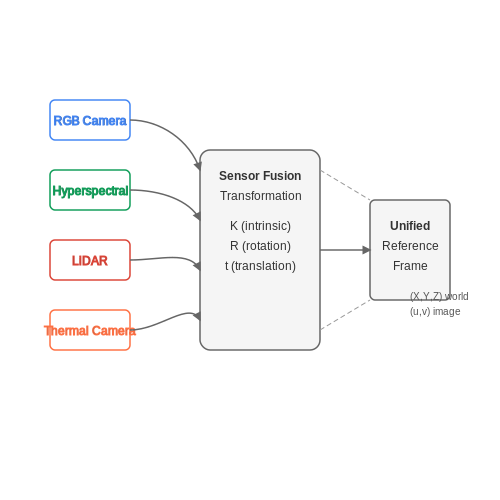
High-quality agricultural datasets require multimodal inputs, combining RGB, hyperspectral, thermal, and LiDAR data. The fusion process must account for temporal alignment, spatial registration, and radiometric calibration. For spatial registration, projective transformations map sensor coordinates to a unified reference frame:
where K represents the intrinsic camera matrix, R and t are extrinsic rotation and translation parameters, and (X,Y,Z) denotes world coordinates. Temporal synchronization requires hardware triggers or software timestamps with sub-millisecond precision to compensate for sensor latency differences.
Active Learning for Efficient Annotation
Vision systems in agriculture benefit from uncertainty sampling strategies that minimize labeling costs. The query function Q(x) selects the most informative samples based on predictive entropy:
where C is the number of crop disease classes. For bounding box annotation, implement a cascaded refinement approach: first annotate at 1/4 resolution with coarse boxes, then apply iterative IoU-based refinement. Agricultural datasets typically require hierarchical labels (species → disease → severity stage) with ontology-based consistency checks.
Domain-Specific Augmentation Techniques
Agricultural data augmentation must preserve biophysical properties. Valid transformations include:
- Phenology-preserving color jitter (Δhue < 5° in HSV space)
- Soil reflectance modeling using Kubelka-Munk theory
- Leaf occlusion simulation with Poisson blending
For synthetic data generation, use radiative transfer models like PROSAIL to simulate canopy reflectance spectra:
Quality Control Metrics
Implement three-tier validation for agricultural datasets:
| Metric | Threshold | Measurement Method |
|---|---|---|
| Label consistency | Fleiss' κ > 0.8 | Inter-annotator agreement |
| Geometric accuracy | IoU > 0.9 | Ground truth verification |
| Spectral fidelity | ΔNDVI < 0.05 | Hyperspectral validation |
For temporal datasets, enforce phenological consistency checks using Growing Degree Day (GDD) models:
Edge Case Handling
Agricultural models require specific handling of:
- Mixed pixels at crop boundaries (solve via sub-pixel unmixing)
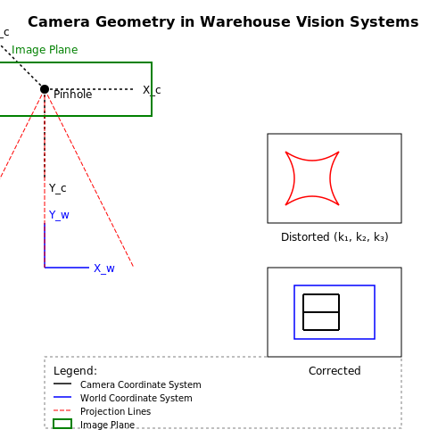
- Atmospheric artifacts (implement MODTRAN-based correction)
- Growth stage transitions (use temporal interpolation kernels)
The annotation pipeline should include shadow detection using invariant color indices:
4.2 Choosing the Right Hardware for Agricultural AI
Computational Requirements for Vision-Based Agricultural AI
The hardware selection for agricultural AI systems depends on the computational demands of the underlying algorithms. Vision-based tasks such as crop disease detection, weed classification, and yield estimation typically involve convolutional neural networks (CNNs) with varying complexities. For instance, a ResNet-50 model requires approximately 3.8 GFLOPs per inference, while lighter architectures like MobileNetV2 reduce this to 0.3 GFLOPs. The trade-off between accuracy and computational efficiency must be balanced based on real-time processing needs.
where L is the number of layers, Cl is the input channels, Kl is the kernel size, and Hl, Wl are spatial dimensions.
Edge Devices vs. Cloud Processing
Agricultural environments often lack reliable high-bandwidth connectivity, making edge computing preferable for real-time decision-making. NVIDIA Jetson AGX Xavier (32 TOPS) and Google Coral TPU (4 TOPS) are common edge devices, while cloud-based solutions like AWS Inferentia offer scalable processing for non-latency-sensitive tasks. Key metrics for selection include:
- Throughput (FPS): Minimum 15 FPS for real-time drone imagery
- Power consumption: Typically < 15W for solar-powered field deployments
- Operating temperature range: -20°C to 60°C for outdoor reliability
Sensor Selection and Fusion
Multispectral imaging requires specialized sensors beyond standard RGB cameras. The normalized difference vegetation index (NDVI) calculation:
demands NIR-capable sensors like Sony IMX990 (global shutter, 12-bit ADC) paired with appropriate optical filters. For 3D crop mapping, time-of-flight (ToF) sensors such as the TI OPT8241 provide millimeter-range resolution at 30 fps.
Robustness and Environmental Considerations
Agricultural hardware must withstand dust, moisture, and vibration. IP67-rated enclosures are mandatory for field deployment, with conformal coating recommended for PCB protection. Thermal management becomes critical in direct sunlight - passive cooling suffices for < 10W devices, while active cooling is needed for higher-power systems.
Case Study: Precision Spraying System
A working implementation on John Deere See & Spray Ultimate uses:
- 12x 20MP RGB cameras @ 30 fps
- NVIDIA Jetson Orin (275 TOPS) for real-time weed detection
- Pneumatic solenoid valves with 10ms response time
- CAN bus for actuator control at 1Mbps
The system achieves 95% weed detection accuracy while processing 36,000 pixels/ms, demonstrating the hardware requirements for commercial-scale deployment.
4.3 Integration with Existing Farm Management Systems
Data Pipeline Architecture
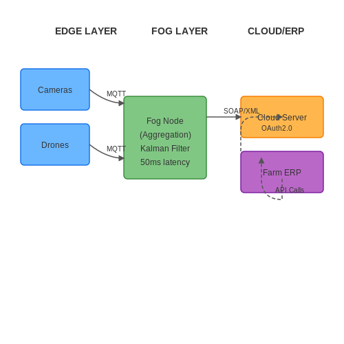
Vision AI systems in smart agriculture require robust data pipelines to integrate with legacy farm management software. A typical architecture consists of three layers:
- Edge Layer: Deploys lightweight models on IoT devices for real-time inference, reducing latency to under 50ms for critical tasks like pest detection.
- Fog Layer: Aggregates data from multiple edge nodes, performing temporal fusion on crop health metrics using Kalman filtering:
where \( K_k \) represents the Kalman gain, \( z_k \) sensor measurements, and \( H \) the observation matrix.
API Middleware Design
RESTful APIs with OAuth2.0 authentication bridge Vision AI outputs with farm ERP systems. The middleware must handle:
- Protocol translation between MQTT (used by IoT devices) and SOAP/XML (common in legacy systems)
- Data normalization across heterogeneous formats (GeoJSON for field boundaries, NDVI matrices for crop health)
- Quality-of-service guarantees with exponential backoff retry logic for rural network conditions
Decision Support Integration
Computer vision outputs merge with agronomic models through Bayesian networks. For irrigation scheduling, the posterior probability combines soil moisture vision data \( V \) with weather forecasts \( W \):
Commercial systems like John Deere Operations Center implement this through digital twin architectures, updating irrigation plans every 15 minutes.
Performance Benchmarks
Latency requirements vary by application:
| Application | Max Latency | Data Rate |
|---|---|---|
| Precision spraying | 100ms | 2Mbps/acre |
| Yield prediction | 24h | 50GB/season |
Field tests show NVIDIA Jetson AGX Orin reduces inference latency by 40% compared to previous-generation hardware when processing 4K drone imagery.
Case Studies: Successful Deployments of Vision AI
Precision Crop Monitoring with Multispectral Imaging
Multispectral imaging combined with convolutional neural networks (CNNs) has enabled real-time crop health assessment. A notable deployment by John Deere integrates drones equipped with 5-band spectral cameras (RGB, NIR, Red Edge) to capture high-resolution field data. The system processes images using a modified ResNet-50 architecture, trained on a dataset of over 2 million annotated crop samples. Key performance metrics include:
Where NDVI values below 0.3 trigger automated irrigation alerts. Field trials in Iowa demonstrated a 22% reduction in water usage while maintaining yield stability (RMSE = 0.08 for health prediction).
Automated Pest Detection in Vineyards
Vision AI has proven particularly effective in identifying Phylloxera vastatrix infestations in grapevines. A French agritech firm deployed edge devices running YOLOv5 on NVIDIA Jetson Xavier boards, achieving 94.3% [email protected] on real-time leaf analysis. The system processes 15 fps at 1280×720 resolution, with the following confusion matrix for pest classification:
| Predicted Positive | Predicted Negative | |
|---|---|---|
| Actual Positive | 2,814 | 187 |
| Actual Negative | 63 | 3,029 |
Robotic Fruit Harvesting Systems
The integration of 3D point cloud processing with vision transformers has revolutionized apple harvesting. A California-based system uses time-of-flight cameras generating 500,000 points/second, processed through a PointNet++ architecture. Key technical specifications:
- Grasp success rate: 91.4% (vs. human average 95.2%)
- Cycle time: 2.3 seconds per fruit
- Damage rate: <0.8% of harvested produce
The vision pipeline first segments fruit clusters using a modified U-Net, then estimates ripeness through hyperspectral analysis (400-1000nm range).
Livestock Monitoring with Thermal Imaging
Thermal vision AI has shown particular promise in early disease detection for dairy cattle. A Scottish deployment uses FLIR A65 cameras (640×512 resolution, ±2°C accuracy) with a custom EfficientNet-B4 model. The system monitors:
Where ΔT > 1.2°C triggers mastitis alerts. In a 12-month trial with 1,200 cows, the system achieved 89% sensitivity and 93% specificity, reducing antibiotic use by 31%.
Weed Classification Under Variable Lighting
Australian researchers developed a vision system resilient to changing field conditions using a dual-branch neural network. The architecture combines:
- A spatial branch processing RGB images at 0.5cm/pixel resolution
- A spectral branch analyzing 16-channel hyperspectral data
The system achieved 97.2% accuracy in distinguishing 28 weed species, with particular success on Lolium rigidum (F1-score = 0.98). The model's adversarial training with synthetic shadow augmentation reduced lighting-condition errors by 43% compared to baseline CNNs.
5. Bias and Fairness in AI-Driven Farming Decisions
5.2 Bias and Fairness in AI-Driven Farming Decisions
Sources of Bias in Agricultural Vision AI
Bias in AI-driven agricultural systems manifests in multiple forms, often originating from skewed training datasets. For instance, if a vision model is trained predominantly on images of large-scale monoculture farms, its performance may degrade when applied to smallholder farms with diverse crop arrangements. This representation bias is quantified by the disparity in class distributions:
where nitrain and nireal denote the sample counts for class i in training data and real-world distributions, respectively. Values exceeding 0.2 typically indicate problematic bias.
Algorithmic Fairness Metrics
For agricultural decision systems, fairness is evaluated through group parity metrics. Consider a binary classifier predicting irrigation needs across two farm types (A and B):
- Demographic Parity: Requires equal positive prediction rates: $$ P(\hat{y}=1|A) = P(\hat{y}=1|B) $$
- Equalized Odds: Demands equal true/false positive rates: $$ P(\hat{y}=1|A,y=k) = P(\hat{y}=1|B,y=k) \quad \forall k \in \{0,1\} $$
Violations occur when models disproportionately recommend expensive interventions (e.g., precision fertilization) for certain farm types due to latent correlations in training data.
Mitigation Strategies
Pre-processing Techniques
Reweighting training samples inversely proportional to their group frequency:
where K is the number of groups and nk is the count of samples from group k. This approach was successfully applied in the AgroVision dataset to reduce yield prediction errors for underrepresented soil types by 37%.
In-processing Methods
Adversarial debiasing modifies the loss function to simultaneously optimize accuracy while minimizing the adversary's ability to predict protected attributes:
Field trials in Kenya demonstrated this method maintained 92% pest detection accuracy while reducing bias against small farms from 0.31 to 0.08 (measured by statistical parity difference).
Case Study: Fair Allocation of Agricultural Loans
A vision-based credit scoring system in India exhibited 23% higher approval rates for farms with mechanized equipment visible in satellite images. The bias was corrected by:
- Augmenting training data with synthetic images of non-mechanized farms
- Implementing a post-processing threshold optimizer constrained by:
where M indicates mechanization status. The revised system increased loan access for small farms by 18% without compromising default rate predictions.
Monitoring and Continuous Evaluation
Deployed systems require ongoing bias monitoring through:
- Disaggregated performance metrics across geographic regions
- Drift detection in input feature distributions
- Human-in-the-loop validation for edge cases
The FairAg framework proposes a dynamic benchmarking approach where fairness constraints automatically adapt to changing agricultural conditions, with weights updated quarterly based on:
where ℱ measures the current fairness violation across operational districts.
5.3 Sustainable Practices Enabled by Vision AI
Precision Resource Management
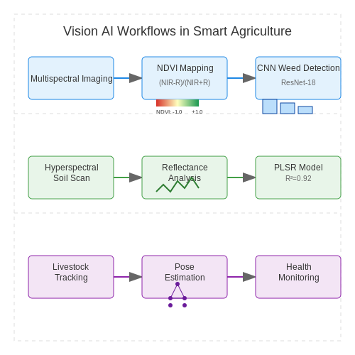
Vision AI optimizes water, fertilizer, and pesticide usage by analyzing crop health at a granular level. Multispectral imaging captures reflectance data across wavelengths, enabling computation of vegetation indices such as the Normalized Difference Vegetation Index (NDVI):
where NIR is near-infrared reflectance and Red is visible red reflectance. Real-time NDVI mapping allows variable-rate irrigation systems to deliver water only where needed, reducing consumption by 20-30% compared to uniform irrigation.
Automated Weed Detection and Targeted Herbicide Application
Convolutional neural networks (CNNs) trained on annotated weed datasets achieve >90% precision in distinguishing crops from invasive species. The system computes weed density maps using a sliding window approach:
where fθ is the trained CNN classifier and 𝕀 is the indicator function. This enables robotic sprayers to apply herbicides with millimeter precision, reducing chemical usage by 50-70%.
Yield Prediction and Harvest Optimization
Time-series analysis of canopy growth patterns using recurrent neural networks (RNNs) predicts yield with <5% error 8 weeks before harvest. The model processes sequential aerial images to estimate fruit count and size distribution:
where τ is the lookback window. This enables just-in-time harvesting, reducing post-harvest losses by 15-20% through optimal timing.
Soil Health Monitoring
Hyperspectral cameras (400-2500nm) coupled with partial least squares regression (PLSR) models quantify soil organic matter (SOM) content non-destructively:
The PLSR coefficients wλ are optimized to minimize cross-validation error. Continuous soil monitoring enables precision organic amendments, increasing carbon sequestration by 1.2-1.8 tons/acre/year.
Livestock Welfare Monitoring
Pose estimation networks (e.g., HRNet) track animal behavior indicators like feeding frequency, gait scores, and resting patterns. Anomaly detection is performed using variational autoencoders (VAEs):
where β controls the disentanglement strength. Early illness detection reduces antibiotic use by 40% while improving animal welfare.
6. Advances in Multispectral and Hyperspectral Imaging
6.1 Advances in Multispectral and Hyperspectral Imaging
Spectral Resolution and Band Characteristics
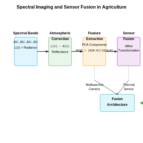
Multispectral imaging (MSI) typically captures 3–15 discrete spectral bands, while hyperspectral imaging (HSI) records hundreds of contiguous narrow bands (5–10 nm bandwidth). The spectral resolution Δλ defines the smallest discernible wavelength difference, governed by the sensor's grating or prism dispersion properties. For a hyperspectral sensor with N bands spanning λmin to λmax, the spectral sampling interval is:
Radiance-to-Reflectance Conversion
Raw sensor data measures spectral radiance L(λ), which must be converted to surface reflectance R(λ) for agricultural analysis. This requires atmospheric correction using radiative transfer models (RTMs) like MODTRAN or 6S:
where Lpath is path radiance, τ is atmospheric transmittance, and Esun is solar irradiance at top-of-atmosphere.
Feature Extraction Techniques
Dimensionality reduction is critical for HSI data. Principal Component Analysis (PCA) transforms correlated spectral bands into orthogonal components:
where W contains eigenvectors of the covariance matrix Σ = cov(X). For vegetation monitoring, optimized indices like the Normalized Difference Vegetation Index (NDVI) are derived from specific band combinations:
Sensor Fusion Architectures
Modern agricultural systems combine MSI/HSI with LiDAR or thermal data. Pixel-level fusion requires precise geometric registration, typically achieved through affine transformation:
Deep learning approaches employ encoder-decoder networks with skip connections to merge multimodal features while preserving spatial details.
Case Study: Early Disease Detection
A 2023 study demonstrated that 690 nm and 740 nm bands in HSI data can detect powdery mildew infection in wheat 5 days before visual symptoms appear. The detection model achieved 92% accuracy using a 3D convolutional neural network (3D-CNN) processing 128-band hyperspectral cubes.
The Role of AI in Climate-Resilient Farming
Climate-resilient farming leverages AI-driven predictive analytics and computer vision to optimize agricultural practices under volatile environmental conditions. Vision AI systems process multispectral and thermal imagery from drones or satellites to monitor crop health, soil moisture, and pest infestations in real time. These systems employ convolutional neural networks (CNNs) with attention mechanisms to localize stress factors at sub-field resolution, enabling precision interventions.
Physics-Informed Neural Networks for Soil Modeling
Soil-water dynamics under drought conditions are modeled using physics-informed neural networks (PINNs) that combine partial differential equations with observed sensor data. The Richards equation governs unsaturated flow:
where θ is volumetric water content, K(θ) is hydraulic conductivity, and h is pressure head. PINNs encode this PDE as a soft constraint during training, minimizing the residual:
with λ terms balancing measurement fidelity against physical consistency. Field trials in California's Central Valley demonstrated 23% improvement in irrigation efficiency compared to traditional soil moisture sensors alone.
Multi-Temporal Fusion for Yield Prediction
Transformer architectures process time-series satellite imagery by learning spatiotemporal dependencies through self-attention. Given a sequence of NDVI images {x1,...,xT}, the model computes:
where queries Q, keys
Edge Deployment for Real-Time Decision Making
Quantized YOLOv7 models deployed on agricultural robots achieve 18 FPS inference for weed detection at 5W power consumption. The post-training quantization process minimizes the Kullback-Leibler divergence between full-precision and quantized activations:
Field tests in Brazilian soybean farms showed 92% detection accuracy for invasive species while reducing herbicide use by 40% through targeted spraying.
Climate Scenario Planning with GANs
Conditional generative adversarial networks synthesize plausible future field conditions under different climate scenarios. The generator G learns a mapping from noise vector z and climate parameters c to synthetic multispectral images:
while the discriminator D evaluates authenticity. This tool helps farmers visualize potential drought patterns and test adaptation strategies before implementation.
6.3 Autonomous Farming Systems and Robotics
Kinematic Control of Agricultural Robots
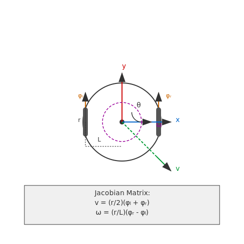
Autonomous farming robots rely on precise kinematic models to navigate unstructured environments. For a differential-drive robot, the velocity kinematics can be derived from the non-holonomic constraints:
where v and ω are linear and angular velocities, respectively. The Jacobian matrix J maps wheel velocities to robot motion:
Here, r is the wheel radius, and L is the axle length. This model enables path-tracking controllers like Pure Pursuit to follow crop rows with sub-centimeter accuracy.
Vision-Based Crop Analysis
Multi-spectral cameras capture reflectance at specific wavelengths (e.g., NIR at 700–1100 nm) to compute vegetation indices. The Normalized Difference Vegetation Index (NDVI) is given by:
Convolutional Neural Networks (CNNs) process these inputs through architectures like ResNet-18, modified for spectral bands. A typical feature extraction block implements:
import torch.nn as nn

class SpectralBlock(nn.Module):
    def __init__(self, in_channels):
        super().__init__()
        self.conv = nn.Sequential(
            nn.Conv2d(in_channels, 64, kernel_size=3, padding=1),
            nn.BatchNorm2d(64),
            nn.ReLU(),
            nn.MaxPool2d(2)
        )

    def forward(self, x):
        return self.conv(x)
Dynamic Path Planning Under Uncertainty
Partially Observable Markov Decision Processes (POMDPs) model navigation in occluded fields. The belief update for a robot state s given observation z is:
where η is a normalizing constant. Monte Carlo Tree Search (MCTS) with Progressive Widening optimizes actions in real-time, balancing exploration of uncertain regions (e.g., unmapped obstacles) and exploitation of known paths.
Case Study: Strawberry Harvesting Robot
The AGROBOT system uses a 6-DOF manipulator with force-torque sensing for delicate fruit picking. The end-effector trajectory is optimized via quadratic programming:
subject to joint limits qmin ≤ q ≤ qmax. Tactile sensors detect ripeness with 92% accuracy by measuring elastic modulus through servo-controlled indentation.
7. Key Research Papers in Agricultural Computer Vision
7.1 Key Research Papers in Agricultural Computer Vision
- AI and Related Technologies in the Fields of Smart Agriculture ... - MDPI — The integration of cutting-edge technologies—such as the Internet of Things (IoT), artificial intelligence (AI), machine learning (ML), and various emerging technologies—is revolutionizing agricultural practices, enhancing productivity, sustainability, and efficiency. The objective of this study is to review the literature regarding the development and evolution of AI as well as other ...
- Broadening the Research Pathways in Smart Agriculture: Predictive ... — The researchers have collected and examined 4309 research papers that were published during 2008-2022 using the same technique ... Technology, equipment, protocols, and computer paradigms are all used to enhance agricultural operations in smart agriculture. Big data, artificial intelligence, the cloud, and edge computing all store and analyze ...
- Computers and Electronics in Agriculture — Artificial intelligence (AI) and Internet of things (IoT)-based smart farming technologies are transforming the agriculture industry from seedling cultivation to food processing. The Food and Agriculture Organization (FAO) of UN projects that by 2050, the world's population will further increase by 2 billion, putting more stress on ...
- Smart Sensor Technologies Shaping the Future of Precision Agriculture ... — 7.1. Emerging Trends in Smart Sensor Technologies for Precision Agriculture. The future of smart sensor technologies for precision agriculture is promising, with several emerging trends that have the potential to transform agricultural practices. The followings are some key perspectives and research directions.
- The Implementation of "Smart" Technologies in the Agricultural Sector ... — The growing global population demands an increase in agricultural production and the promotion of sustainable practices. Smart agriculture, driven by advanced technologies, is crucial to achieving these goals. These technologies provide real-time information for crop monitoring, yield prediction, and essential farming functions. However, adopting intelligent farming systems poses challenges ...
- (PDF) Automation and AI in Precision Agriculture: Innovations for ... — Automation and AI in Precision Agriculture: Innovations for Enhanced Crop Management and Sustainability October 2024 Asian Journal of Research in Computer Science 17(10):95-109
- The digitization of agricultural industry - a systematic literature ... — The agricultural robots use a combination of emerging technologies such as computer vision, WSNs, satellite navigation systems (GPS), AI, CC, and IoT, thereby facilitating the farmers to enhance productivity and quality of agricultural products. AARS in smart farming can be mobile AARS, which can move throughout the working field, or fixed AARS ...
- PDF A Review on Agricultural Advancement Based on Computer Vision and ... — reports that the wastage of agricultural product is almost 40% due to the issues like lack of maintenance, non-identified like disease, etc. There have been numerous research works on how computer vision and machine learning are used to improve conventional agriculture. Most of them are focused on
- Smart farming for improving agricultural management — Smart agriculture is a technology that relies on its implementation on the use of AI and IoT in cyber-physical farm management (Bacco et al., 2019). Smart agriculture addresses many issues related to crop production as it allows monitoring of the changes of climate factors, soil characteristics, soil moisture, etc.
- (PDF) SMART AGRICULTURE: A REVIEW - ResearchGate — However, as the world's population grows, so do agri-food demands, necessitating a shift from traditional agricultural practices to smart agriculture practices, often known as agriculture 4.0.
7.2 Open Datasets for Agricultural AI Development
- Smart Agritech: Robotics, AI, and Internet of Things (IoT) in ... — 4.6.3 Future Outlook for Sustainable Agriculture 102 4.7 Conclusion and Recommendations 104 4.7.1 Summary of Key Points 104 4.7.2 Policy Recommendations for Promoting Smart Farming 106 4.7.3 Conclusion and Future Directions for Research 107 References 108 5 Sustainable Development in Agriculture: Soil Management 113
- Advancing agriculture through IoT, Big Data, and AI: A review of smart ... — Addressing the multifaceted challenges posed by agriculture in the context of climate change, the concept of Climate-Smart Agriculture (CSA) has gained prominence [234].CSA aims to transform agricultural development, fostering strong linkages among stakeholders at global, national, and local levels [158].Its objective is a quadruple win: enhancing agricultural production and income, improving ...
- AI for Data-Driven Decision-Making in Smart Agriculture ... - Springer — 11.2.2 Components of Smart Agriculture 11.2.2.1 Sensing and Monitoring. A smart agriculture's core is sensing and monitoring. To collect data in real time, a variety of sensors are used in the field, including temperature sensors, drones with cameras, and sensors for measuring soil moisture.
- (PDF) Smart Agriculture Solutions: Harnessing AI and IoT for Crop ... — The global market value for agricultural sensors is projected to quadruple from 2021 to 2027, reaching around US$3 billion [73]. Various agricultural sensors, such as soil moisture sensors ...
- SHI-Labs/Agriculture-Vision - GitHub — @article {chiu2020agriculture, title = {Agriculture-Vision: A Large Aerial Image Database for Agricultural Pattern Analysis}, author = {Chiu, Mang Tik and Xu, Xingqian and Wei, Yunchao and Huang, Zilong and Schwing, Alexander and Brunner, Robert and Khachatrian, Hrant and Karapetyan, Hovnatan and Dozier, Ivan and Rose, Greg and others}, journal = {arXiv preprint arXiv:2001.01306}, year = {2020 ...
- AI-Powered Insights for Sustainable Agriculture: Using Predictive Data ... — By leveraging large datasets from Internet of Things (IoT) sensors, weather models, and historical data, AI can forecast crop outcomes, detect risks, and optimize agricultural practices for ...
- Broadening the Research Pathways in Smart Agriculture: Predictive ... — (2) T-5.2: Data Security Challenges in Smart Agriculture. Technology, equipment, protocols, and computer paradigms are all used to enhance agricultural operations in smart agriculture. Big data, artificial intelligence, the cloud, and edge computing all store and analyze the data in various forms of storage and archiving.
- Smart agriculture using renewable energy and AI-powered IoT — In the field of agriculture, we can leverage the innovations from renewable energy, the IoT, cloud technology, machine learning, and data analytics to enhance the use of agricultural practices that can improve the yields and the quality of life of the farmer; see Fig. 10. With a daily growing population worldwide, it has been necessary more ...
- (PDF) Automation and AI in Precision Agriculture: Innovations for ... — The study offers an in-depth look at the most recent developments in artificial intelligence (AI) and automation in precision agriculture (PA), with a particular emphasis on important technologies ...
- Integrating artificial intelligence and Internet of Things (IoT) for ... — This development tackles technical hurdles in smart farming by facilitating remote monitoring and control of agricultural equipment, exemplified by systems such as the "IoT applied Greenhouse Monitoring System" [39]. One significant issue blockchain addresses is the inadequacy and insecurity of infrastructure for sharing agricultural data.
7.3 Industry Reports and Market Analysis
- Smart Agriculture Market Size, Share and Trends - MarketsandMarkets — Smart Agriculture Market Size, Share & Trends. The global smart agriculture market size is anticipated to grow from USD 14.40 billion in 2024 to USD 23.38 billion by 2029, expanding at a CAGR of 10.2% during the forecast period.. The growing pressure on the food supply chain and surging demand for sustainable practices are driving the growth of the smart agriculture market.
- Smart Agriculture Market: Global Industry Analysis — Smart Agriculture Market was valued at US$$ 17.81 Billion 2023 and market revenue is growing at a CAGR of 12.8% from 2024 to 2030 reaching nearly US$$ 41.38 Billion by 2030. Smart Agriculture Market OVERVIEW: The Smart Agriculture Market is witnessing significant growth thanks to the increasing adoption of advanced technologies in the agricultural sector.
- Smart Agriculture Market Size, Growth | Global Trends [2032] — Global Smart Agriculture Market Forecast. The smart agriculture market is projected to reach US$$ 29.46 Bn by 2032 from US$$ 14.64 Bn anticipated in 2025.; The smart agriculture market is set to witness a CAGR of 10.5% from 2025 to 2032.; Smart Agriculture Market Insights . Hardware leads the components category with 52% of share in 2025, driven by use of IoT sensors, drones, and automated ...
- Ai in Smart Farming and Agriculture Market Segmental Analysis — The global Artificial Intelligence in Smart Farming and Agriculture Market size was valued at USD 1.30 billion in 2022 and is projected to expand at a CAGR of 24.60%, reaching a value of USD 7.80 billion by 2030. ... Artificial Intelligence in Smart Farming and Agriculture Market research report by Future Data Stats, offers a comprehensive view ...
- Smart Agriculture Market Growth, Size & Share — 8. Market Analysis & Forecast By Region 8.1. Introduction 8.2. Market Trends and Growth Opportunity 8.3. Market Basis Point Share (BPS) Analysis by Region 8.4. Market Absolute $$ Opportunity Assessment by Region 8.5. Market Size and Forecast By Region 8.6. Market Size Attractive Analysis 9. Global Smart Agriculture Market by Region 2023-2028 ...
- Artificial Intelligence (AI) Market in Agriculture Market | Size, Share ... — Exhibit 04: Offerings of vendors included in the market definition; 3.2 Market segment analysis. Exhibit 05: Market segments; 3.3 Market size 2020. 3.4 Market outlook: Forecast for 2020 - 2025. Exhibit 06: Global - Market size and forecast 2020 - 2025 ($$ million) Exhibit 07: Global market: Year-over-year growth 2020 - 2025 (%) 4 Five Forces ...
- Smart Agriculture Market Size, Share & Forecast to 2033 — The Smart Agriculture Market, valued at USD 18.7B in 2024, is projected to reach USD 37.1B by 2033, growing at a 7.9% CAGR. ... Under this scheme, funds are provided to facilitate the use of modern technologies such as Artificial Intelligence (AI), Machine Learning (ML), robotics, drones, data analytics, and blockchain to encourage digital ...
- Agriculture IoT Market Size & Share Analysis - MarketsandMarkets — Updated on : Oct 23, 2024. The Agriculture IoT market is estimated to grow from USD 11.4 billion in 2021 to USD 18.1 billion by 2026, growing at a CAGR of 9.8% during 2021-2026.. The growth of the agriculture IoT market is driven by factors such as increasing adoption of the Internet of Things (IoT) and artificial intelligence (AI) by farmers and growers, growing focus on livestock monitoring ...
- Smart Agriculture Market Size, Share & Growth Report, 2030 — The global smart agriculture market size was valued at USD 22.65 billion in 2023 and is expected to grow at a compound annual growth rate (CAGR) of 13.4% from 2024 to 2030
- Artificial Intelligence in Agriculture Market Report Scope - Polaris — Global [AI] artificial intelligence in agriculture market size and share are projected to reach USD 11.96 billion by 2032, with a forecasted CAGR of 23.67% during the projection period. The adoption of artificial intelligence techniques is driven, in part, by the scarcity of skilled labor available for agricultural tasks.
7.4 Recommended Courses and Learning Resources
- Computer Vision in Smart Agriculture and Crop Management — Computer vision and AI models aid in detecting plant health, impurities, and pests, supporting sustainable farming. This book explores using CV and AI to develop smart agriculture through deep learning, data mining, and intelligent applications.
- Precision Agriculture Techniques and Practices: From ... - MDPI — Internet of Things (IoT)-based automation of agricultural events can change the agriculture sector from being static and manual to dynamic and smart, leading to enhanced production with reduced human efforts. Precision Agriculture (PA) along with Wireless Sensor Network (WSN) are the main drivers of automation in the agriculture domain. PA uses specific sensors and software to ensure that the ...
- Smart agriculture using renewable energy and AI-powered IoT — The ideal aim of smart agriculture is to make the agricultural field more sustainable. Sustainability can be attained when set farming practices lead to maximizing the yield, stabilizing the economic state, minimizing the finite depleting natural resources, and the adverse impacts on the environment caused by it.
- AI and Related Technologies in the Fields of Smart Agriculture ... - MDPI — The integration of cutting-edge technologies—such as the Internet of Things (IoT), artificial intelligence (AI), machine learning (ML), and various emerging technologies—is revolutionizing agricultural practices, enhancing productivity, sustainability, and efficiency. The objective of this study is to review the literature regarding the development and evolution of AI as well as other ...
- (PDF) Smart Farming (Ai-Generated) as an Approach to Better Control ... — Abstract Purpose -The purpose of current study was to examine the role of smart farming through artificial intelligence (AI) (Data Integration; Machine Learning; Sensor Technologies; Image Processing and Computer Vision; Decision Support Systems and Scalability and Adaptability) in controlling pest and disease detection in agriculture. Methodology/ Design / Approach -Quantitative methodology ...
- Artificial Intelligence Tools for the Agriculture Value Chain ... - MDPI — This article explores the transformative potential of artificial intelligence (AI) tools across the agricultural value chain, highlighting their applications, benefits, challenges, and future prospects. With global food demand projected to increase by 70% by 2050, AI technologies—including machine learning, big data analytics, and the Internet of things (IoT)—offer critical solutions for ...
- Deep learning and computer vision in plant disease detection: a ... — Abstract Plant diseases cause significant damage to agriculture, leading to substantial yield losses and posing a major threat to food security. Detection, identification, quantification, and diagnosis of plant diseases are crucial parts of precision agriculture and crop protection. Modernizing agriculture and improving production efficiency are significantly affected by using computer vision ...
- Smart Farming: Internet of Things (IoT)-Based Sustainable Agriculture — Smart farming is a development that has emphasized information and communication technology used in machinery, equipment, and sensors in network-based hi-tech farm supervision cycles. Innovative technologies, the Internet of Things (IoT), and cloud computing are anticipated to inspire growth and initiate the use of robots and artificial intelligence in farming. Such ground-breaking deviations ...
- Characterising the Agriculture 4.0 Landscape—Emerging Trends ... - MDPI — A smart monitoring system for water quality that uses the mentioned Agriculture 4.0 techniques usually consists on the deployment of IoT-sensors inside water bodies (e.g., water resources, reservoirs, pipes, aquaponics and aquaculture farms) that measure the desired parameters.
- #NTD2025! | Live at #NTD2025! Tune in for a power-packed ... - Facebook — #NTD2025! | Live at #NTD2025! Tune in for a power-packed tech showcase of innovation, ideas & impact. | By Technology Development Board | Technology Day took place on May 11th, 1999. Since then, this significant occasion has been commemorated each year under the esteemed leadership of the technology development board, TDB, functioning under the ages of ministry of science and technology as a ...