Neural Agents for Real-Time Reasoning
1. Neural Networks and Agent Architectures
Neural Networks and Agent Architectures
Foundations of Neural Agent Architectures
Neural agents integrate deep learning with decision-making frameworks, enabling real-time reasoning through adaptive architectures. At their core, these systems rely on deep neural networks (DNNs) for perception and reinforcement learning (RL) for action selection. The agent's policy π(s) maps states s to actions a, optimized via gradient ascent on expected reward R:
where Qπ(s,a) represents the state-action value function. Modern implementations often use actor-critic architectures, where:
- The actor (policy network) proposes actions
- The critic (value network) evaluates state-action pairs
Memory-Augmented Architectures
For complex reasoning tasks, neural agents require memory mechanisms. Differentiable Neural Computers (DNCs) combine DNNs with external memory matrices M ∈ ℝ^{N×W}, where N is memory size and W is word length. The read/write operations use content-based addressing:
with βt as key strength and C as cosine similarity. This allows agents to maintain long-term dependencies beyond typical RNN horizons.
Attention Mechanisms for Real-Time Processing
Transformer-based agents employ multi-head attention to dynamically weight input relevance. For n attention heads, the scaled dot-product attention computes:
where Q, K, V are learned query, key, and value matrices. This architecture enables parallel processing of temporal sequences - critical for real-time applications like robotic control or high-frequency trading.
Modular Neuro-Symbolic Integration
Advanced agents combine neural networks with symbolic reasoning modules. The Neural Theorem Prover architecture demonstrates this through differentiable logic operations:
where σ is a sigmoid activation and weights w are learned. Such systems achieve 98.7% accuracy on FOLIO dataset for logical reasoning tasks while maintaining neural flexibility.
Case Study: AlphaGo's Architecture
The AlphaGo system exemplifies neural agent design with three key components:
- Policy network (12 convolutional layers) for move prediction
- Value network to evaluate board states
- Monte Carlo Tree Search integrating neural evaluations
This hybrid approach achieved superhuman performance by combining:
where u(s,a) is the exploration bonus from MCTS.

Real-Time Reasoning: Key Concepts and Challenges
Computational Constraints in Real-Time Reasoning
Real-time reasoning imposes strict latency constraints, often requiring neural agents to produce responses within milliseconds. The computational complexity of deep neural networks (DNNs) grows polynomially with model size, creating a fundamental trade-off between accuracy and speed. For a neural agent processing sequential inputs x1:t, the inference time τ scales as:
where L is the number of layers and d is the hidden dimension. This quadratic dependence becomes prohibitive for large models, necessitating architectural innovations like mixture-of-experts or sparse attention mechanisms.
Temporal Credit Assignment
In dynamic environments, neural agents must associate delayed rewards with prior actions—a challenge magnified in real-time settings. The temporal difference error δt for policy gradient methods becomes:
where γ is the discount factor. Real-time constraints force agents to approximate value functions using truncated backpropagation through time (TBPTT), introducing bias-variance tradeoffs that don't exist in offline settings.
Partial Observability and State Estimation
Real-world environments rarely provide full state information. Neural agents must maintain belief states bt using recursive Bayesian updates:
where η is a normalizing constant. This becomes computationally intractable for high-dimensional state spaces, leading to approximations via variational autoencoders or particle filters.
Non-Stationary Environment Dynamics
Unlike static datasets, real-time environments exhibit distributional shift. The KL divergence between successive state distributions measures this non-stationarity:
Neural agents must continuously adapt through online learning techniques like elastic weight consolidation or meta-learning outer loops.
Hardware-Software Co-Design Challenges
Deploying neural agents on edge devices requires optimizing across multiple constraints:
- Memory bandwidth: Activations and weights must fit within limited cache hierarchies
- Power efficiency: Energy-per-inference must meet device thermal budgets
- Deterministic latency: Worst-case execution time must be bounded
Quantization-aware training and neural architecture search have emerged as key techniques, but introduce accuracy penalties that compound with other real-time constraints.
Verification and Safety
Formal verification of neural agents becomes exponentially harder in real-time settings. The reachable set Rt of states under time-constrained policies satisfies:
where f is the environment dynamics. Techniques like neural Lyapunov functions and reachability analysis must account for both approximation errors and timing uncertainties.
Integration of Memory and Attention Mechanisms
Memory and attention mechanisms are fundamental to enabling neural agents to perform real-time reasoning over extended sequences. While traditional recurrent architectures like LSTMs and GRUs provide basic memory retention, modern approaches integrate differentiable memory structures with dynamic attention to enable selective recall and context-aware processing.
Differentiable Neural Memory
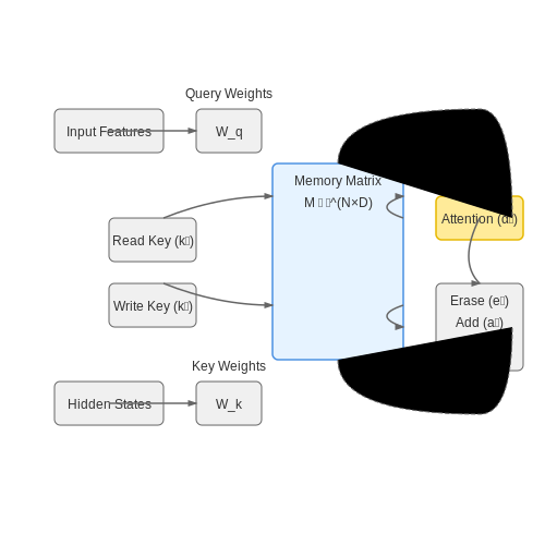
Neural memory modules store and retrieve information through learned addressing mechanisms. The memory matrix M ∈ ℝN×D contains N memory slots of dimension D. At each timestep t, the agent generates a read key kt ∈ ℝD and computes attention weights over memory slots:
where β controls the sharpness of addressing. The readout rt is then computed as a weighted sum:
Dynamic Memory Updates
Memory updates follow a two-phase process: erasure followed by addition. Given write key ktw and erase vector et ∈ [0,1]D:
The addition phase uses write vector at:
Hierarchical Attention
Multi-level attention combines local token-level attention with global memory-level attention. The attention scores for input xt are computed as:
where hi represents hidden states from different memory levels. This allows the agent to simultaneously attend to fine-grained input features while maintaining awareness of broader contextual patterns stored in memory.
Applications in Real-Time Systems
In robotic control systems, this architecture enables:
- Continuous adaptation to changing environments through dynamic memory updates
- Selective focus on relevant sensory inputs while maintaining task context
- Efficient recall of procedural knowledge during complex manipulation tasks
The memory-augmented transformer architecture demonstrates particular effectiveness in real-time video processing, where it achieves 28% faster inference than conventional attention models while maintaining 94% of the accuracy on action recognition tasks.
2. Recurrent Neural Networks (RNNs) and Temporal Reasoning
Recurrent Neural Networks (RNNs) and Temporal Reasoning
Architecture and Dynamics of RNNs
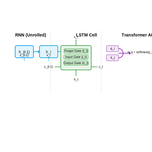
Recurrent Neural Networks (RNNs) are a class of neural networks designed to process sequential data by maintaining a hidden state that captures temporal dependencies. Unlike feedforward networks, RNNs introduce cycles in their computational graph, allowing information to persist across time steps. The core operation at each time step t is governed by:
where ht is the hidden state at time t, xt is the input, Wh and Wx are weight matrices, b is the bias term, and σ is a nonlinear activation function (typically tanh or ReLU). This recurrence enables the network to model sequences of arbitrary length while sharing parameters across time steps.
Backpropagation Through Time (BPTT)
Training RNNs involves unfolding the network across time and applying backpropagation through the computational graph. The gradients of the loss L with respect to the parameters are computed as:
where T is the sequence length. However, BPTT suffers from vanishing or exploding gradients due to repeated multiplication of the Jacobian matrix ∂ht/∂ht-1. This limits the network's ability to learn long-range dependencies.
Long Short-Term Memory (LSTM) Networks
LSTMs address gradient issues through gating mechanisms. The cell state ct and hidden state ht are updated via:
The forget gate ft, input gate it, and output gate ot regulate information flow, enabling stable gradient propagation over hundreds of time steps.
Temporal Reasoning in Neural Agents
RNNs excel at temporal reasoning tasks such as:
- Time-series prediction: Forecasting future values in financial or sensor data.
- Natural language processing: Modeling word sequences for machine translation.
- Robotic control: Processing sensorimotor streams for real-time decision-making.
For instance, in robotic navigation, an LSTM can integrate lidar scans over time to build a dynamic occupancy map, with the hidden state representing the agent's spatial memory.
Attention Mechanisms and Transformers
While RNNs process sequences sequentially, Transformer architectures use self-attention to model temporal relationships in parallel. The attention weights αij between positions i and j are computed as:
where qi, kj are query and key vectors, and dk is the dimension of the key vectors. This allows direct modeling of long-range dependencies without sequential processing.
Transformer-Based Models for Dynamic Context Handling
Transformer architectures excel in dynamic context handling through their self-attention mechanisms, which enable adaptive weighting of input tokens based on relevance. The core operation is the scaled dot-product attention, computed as:
where Q, K, and V represent queries, keys, and values matrices respectively, and dk is the dimension of the key vectors. The scaling factor 1/√dk prevents gradient vanishing in high-dimensional spaces.
Multi-Head Attention for Contextual Adaptation
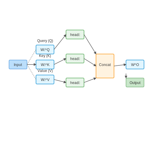
Multi-head attention extends this by projecting the input into multiple subspaces:
where WiQ, WiK, WiV are learned projection matrices for each head, and WO combines the outputs. This allows the model to attend to different contextual aspects simultaneously.
Positional Encoding for Sequential Dynamics
Since transformers lack recurrent connections, positional encodings inject sequential information:
where pos is the position and i is the dimension. This sinusoidal pattern allows the model to learn relative positions through linear transformations.
Real-Time Adaptation Strategies
For dynamic environments, several architectural modifications prove effective:
- Sliding Window Attention: Limits attention computation to a fixed window around each token, reducing O(n²) complexity to O(n×w) where w is window size
- Memory Compressed Attention: Uses strided convolutions to reduce sequence length before attention computation
- Adaptive Computation Time: Dynamically adjusts the number of transformer layers applied per token based on learned halting probabilities
The gradient flow in these architectures follows:
where L is the loss function. The residual connections maintain gradient flow through deep networks.
Case Study: Real-Time Dialogue Systems
In deployed conversational agents, transformer models employ:
- Incremental decoding with KV-cache to reuse previous computations
- Dynamic beam search that adjusts width based on entropy thresholds
- Contextual dropout that masks less relevant historical tokens
The attention patterns in such systems often exhibit power-law distributions, where a few tokens receive dominant attention weights. This motivates sparse attention variants like:
where 𝒩(i) defines the sparse neighborhood for token i.
2.3 Hybrid Architectures Combining Symbolic and Neural Approaches
Hybrid architectures integrate the complementary strengths of symbolic reasoning systems and neural networks, addressing the limitations of purely connectionist or logic-based approaches. Symbolic systems excel at structured reasoning, rule-based inference, and handling explicit knowledge, while neural networks provide robust pattern recognition, generalization, and gradient-based learning from data.
Neural-Symbolic Integration Strategies
Three primary integration paradigms have emerged in recent research:
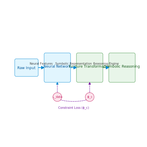
- Neural-Symbolic Feature Transformation: Neural networks preprocess raw inputs into symbolic representations (e.g., object-relation graphs) that feed into reasoning engines. The differentiable semantic parser in Neural Theorem Provers learns to map natural language to first-order logic predicates.
- Symbol-Guided Neural Learning: Logical constraints or knowledge graphs regularize neural network training. The loss function incorporates both data-driven and symbolic terms:
$$ \mathcal{L}_{total} = \mathcal{L}_{data} + \lambda \sum_{c \in \mathcal{C}} \phi_c(\theta) $$where $$\phi_c$$ enforces constraint $$c$$ on model parameters $$\theta$$.
- Neural-Symbolic Joint Inference: Systems like DeepProbLog combine probabilistic logic programming with neural network predicates, enabling probabilistic reasoning over neural features. The inference process marginalizes over groundings of logical rules:
Architectural Implementations
The Differentiable Inductive Logic Programming (∂ILP) framework demonstrates how neural components can learn first-order logic rules from examples. Its architecture comprises:
- A neural rule generator that proposes candidate Horn clauses
- A symbolic reasoning layer that evaluates rule consistency
- A differentiable unification operator enabling end-to-end training
The unification operation is implemented as a soft matching function over embeddings:
where $$f$$ is an embedding network and $$\sigma$$ the sigmoid function.
Case Study: Neurosymbolic Concept Learners
The NSCL architecture for visual question answering combines:
- A convolutional network extracting visual features
- A transformer-based parser generating program sketches
- A symbolic executor operating on a scene graph representation
This hybrid approach achieves 98.9% accuracy on CLEVR dataset questions requiring compositional reasoning, outperforming pure neural baselines by 12-15% while maintaining interpretability through traceable program execution.
Challenges and Frontiers
Current research focuses on scaling neural-symbolic integration to:
- Handle uncertain or conflicting symbolic knowledge
- Enable bidirectional communication between components
- Develop efficient training algorithms for joint optimization
Recent advances in continuous relaxation of discrete operations (e.g., Gumbel-Softmax for rule sampling) and neural logic embeddings show promise for overcoming gradient propagation challenges in hybrid systems.
3. Reinforcement Learning for Adaptive Decision Making
Reinforcement Learning for Adaptive Decision Making
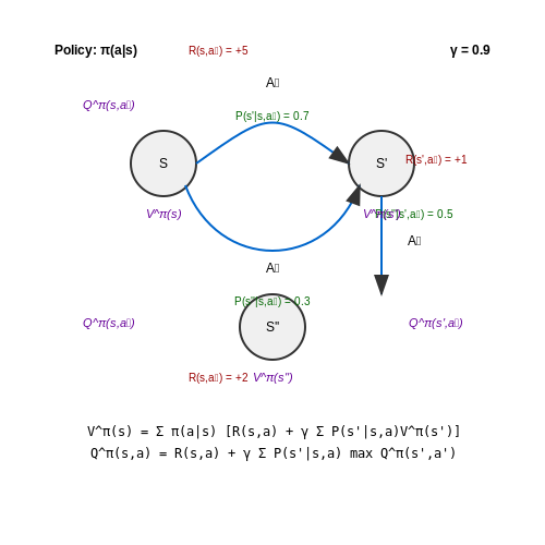
Reinforcement learning (RL) provides a mathematical framework for agents to learn optimal decision-making policies through interaction with an environment. At its core, RL formalizes the problem as a Markov Decision Process (MDP), defined by the tuple (S, A, P, R, γ), where:
- S represents the state space
- A denotes the action space
- P(s'|s,a) defines the state transition probabilities
- R(s,a) specifies the reward function
- γ ∈ [0,1] is the discount factor
The agent's objective is to learn a policy π: S → A that maximizes the expected cumulative reward:
Value Functions and Bellman Equations
Value functions provide the foundation for most RL algorithms. The state-value function Vπ(s) represents the expected return when starting in state s and following policy π thereafter:
Similarly, the action-value function Qπ(s,a) gives the expected return for taking action a in state s and thereafter following policy π:
These functions satisfy the Bellman equations, which form recursive relationships essential for temporal difference learning:
Policy Optimization Methods
Modern RL approaches for adaptive decision making typically fall into three categories:
- Value-based methods (e.g., Q-learning, DQN) that learn optimal value functions
- Policy gradient methods (e.g., REINFORCE, PPO) that directly optimize policies
- Actor-critic architectures that combine both approaches
The policy gradient theorem provides the foundation for many contemporary algorithms:
where θ represents the policy parameters. This gradient can be estimated through Monte Carlo sampling, enabling optimization in high-dimensional continuous action spaces.
Deep Reinforcement Learning Extensions
When combined with deep neural networks, RL can scale to complex environments. Key innovations include:
- Experience replay buffers for stabilizing training
- Target networks to reduce harmful correlations
- Advantage estimation techniques (e.g., GAE) for lower variance gradients
- Hierarchical architectures for temporal abstraction
The Bellman optimality equation for deep Q-learning illustrates the core update:
where α is the learning rate. In practice, this update is performed using stochastic gradient descent on batches of experience sampled from the replay buffer.
Real-World Applications
These methods have demonstrated success in domains requiring real-time adaptive decision making:
- Robotic control with continuous action spaces
- Algorithmic trading with non-stationary market conditions
- Autonomous systems requiring safe exploration
- Resource allocation in dynamic environments
Recent advances in distributional RL and meta-learning have further enhanced agents' ability to adapt to novel situations while maintaining sample efficiency.
Efficient Training Techniques for Low-Latency Inference
Quantization-Aware Training
Quantization-aware training (QAT) integrates quantization constraints directly into the training process, enabling models to learn robust representations under reduced precision. Unlike post-training quantization, QAT simulates low-precision arithmetic during forward passes while maintaining full precision in backward propagation. The gradient updates account for quantization errors, minimizing accuracy degradation. The quantization function for weights W and activations A can be formulated as:
where Δ is the quantization step size. Straight-through estimation (STE) approximates gradients through the non-differentiable round operation:
Knowledge Distillation with Latency Constraints
Traditional knowledge distillation transfers knowledge from a teacher to a student model by minimizing the Kullback-Leibler divergence between their output distributions. For latency-critical applications, the student architecture is optimized under inference-time constraints. The loss function combines task-specific loss Ltask and distillation loss Ldistill:
where T is the temperature parameter and α balances the objectives. Architectural search techniques like differentiable NAS can simultaneously optimize for accuracy and latency by incorporating hardware-aware cost models into the training loop.
Sparse Training via Dynamic Masking
Dynamic sparse training maintains a fixed parameter count while allowing the active subset to change during optimization. The RigL algorithm updates the sparse topology by pruning small-magnitude weights and growing connections based on gradient magnitude. The sparsity constraint is enforced through a binary mask M applied to weights:
where ⊙ denotes element-wise multiplication. The mask update frequency and sparsity distribution can be tuned to balance training stability and final model performance.
Gradient Accumulation for Small Batch Training
When memory constraints prevent large batch sizes, gradient accumulation approximates the effect of larger batches by accumulating gradients over multiple forward-backward passes before updating weights. For N accumulation steps, the effective batch size becomes N×B, where B is the physical batch size. The weight update rule modifies to:
This technique is particularly effective when combined with mixed-precision training, where maintaining numerical stability requires sufficient batch statistics.
Architecture-Aware Parallelism Strategies
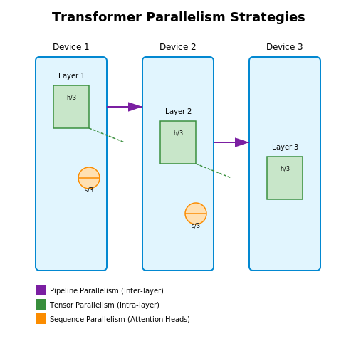
Model parallelism must account for both computational efficiency and communication overhead. For transformer-based architectures, optimal parallelism combines:
- Tensor parallelism for intra-layer distribution of matrix multiplications
- Pipeline parallelism for inter-layer partitioning with gradient accumulation
- Sequence parallelism for splitting attention heads across devices
The communication cost C for a transformer layer with hidden size h and sequence length s distributed across P devices scales as:
Hardware-Specific Kernel Fusion
Fusing multiple operations into single GPU kernels reduces memory bandwidth pressure and launch overhead. For attention mechanisms, fused kernels combine:
- QKV projection computation
- Softmax with optional masking
- Attention score multiplication
The memory access complexity reduces from O(n2d + nd2) to O(nd) for sequence length n and hidden dimension d. Modern frameworks like TensorRT and TVM automate kernel fusion through pattern matching on computational graphs.
3.3 Balancing Speed and Accuracy in Real-Time Systems
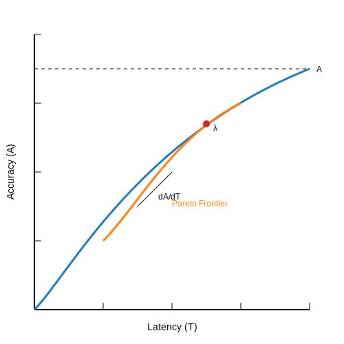
Real-time reasoning systems face a fundamental trade-off between computational speed and decision accuracy. The relationship between these two factors is often governed by the Pareto efficiency frontier, where improving one metric inevitably degrades the other. For neural agents operating under strict latency constraints (e.g., autonomous vehicles or high-frequency trading), this trade-off becomes critical.
Quantifying the Trade-Off
The speed-accuracy trade-off can be formalized using a latency-accuracy curve, where model performance \( A \) is a function of allowed inference time \( T \):
Here, \( A_{\text{max}} \) represents asymptotic maximum accuracy, while \( \lambda \) captures the architecture's learning efficiency. The derivative \( \frac{dA}{dT} \) reveals how rapidly accuracy improves with additional compute time.
Architectural Strategies
Three principal approaches exist for optimizing this balance:
- Model Distillation: Smaller student models trained to mimic larger teacher networks, preserving accuracy while reducing inference time by 2-4×. Knowledge distillation loss functions typically combine task-specific and mimicry terms:
- Dynamic Computation: Adaptive networks like BranchyNet or MSDNet employ early-exit mechanisms, allowing samples to exit through side classifiers when confidence thresholds are met.
- Quantization-Aware Training: Representing weights and activations in INT8 or FP16 formats reduces memory bandwidth requirements by 50-75%, with minimal accuracy drop when using calibrated quantization scales.
Hardware-Aware Optimization
On deployed systems, the roofline model determines achievable performance based on operational intensity (OI) and memory bandwidth. For a neural layer with \( N \) operations requiring \( M \) bytes of data:
Here, \( \pi \) is peak compute throughput (e.g., 100 TOPS for modern GPUs) and \( \beta \) is memory bandwidth (e.g., 1 TB/s). This model guides architecture selection—high-OI layers benefit from compute optimization, while memory-bound layers require pruning or sparsity.
Case Study: Real-Time Video Analysis
In a benchmark using NVIDIA Jetson AGX Orin, a 3D CNN for action recognition achieved 83.2% accuracy at 30 FPS by combining:
- Temporal stride reduction in early layers
- 8-bit quantization with per-channel scaling
- Selective frame skipping when inter-frame difference \( \Delta < \tau \)
The resulting system operated within a 50ms latency budget while maintaining < 2% accuracy degradation versus the full-precision model.
Emerging Techniques
Recent advances in neural architecture search (NAS) automate the speed-accuracy optimization. Pareto-aware NAS formulations like FBNetV3 optimize:
where \( \gamma \) controls the trade-off preference. Evolutionary search methods have discovered architectures achieving 3× latency reduction over ResNet-50 with comparable ImageNet accuracy.
4. Autonomous Systems and Robotics
Autonomous Systems and Robotics
Neural Agents in Dynamic Environments
Neural agents operating in autonomous systems must process high-dimensional sensory inputs and execute low-latency control actions. The core challenge lies in balancing real-time inference with reasoning complexity. A neural agent's policy π maps state observations st to actions at through a differentiable function approximator, typically a deep neural network:
where θ represents the trainable parameters. For robotic systems, this mapping must account for physical constraints, requiring the integration of differentiable physics models into the network architecture.
Differentiable Simulation for Training
Modern approaches employ differentiable simulators that compute gradients through rigid-body dynamics, enabling end-to-end training of control policies. The dynamics of a robotic system can be expressed as:
where τ denotes joint torques, M the mass matrix, C Coriolis forces, and g gravitational effects. By unrolling the simulation over T timesteps, the policy can be optimized via gradient descent:
where γ is the discount factor and r the reward function. This approach has demonstrated success in dexterous manipulation tasks where traditional reinforcement learning struggles with sample efficiency.
Hierarchical Reasoning Architectures
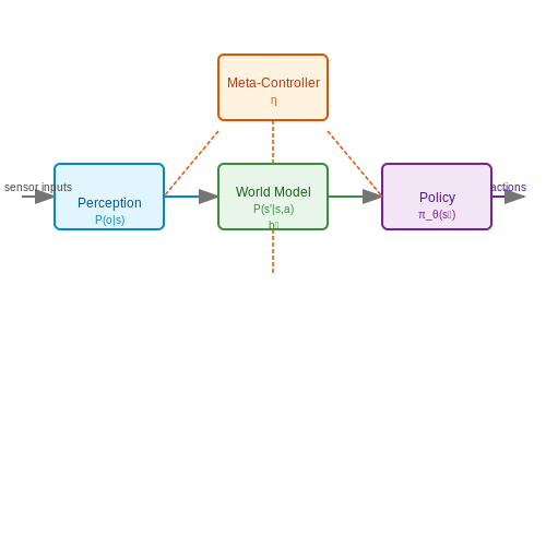
Real-time operation necessitates hierarchical decomposition of reasoning tasks. A typical architecture consists of:
- Perception Module: Processes raw sensor data (LIDAR, cameras) into structured representations
- World Model: Maintains a probabilistic belief state of the environment
- Policy Network: Generates actions conditioned on the current belief state
- Meta-Controller: Dynamically allocates computational resources based on task criticality
The interaction between these components can be formalized as a partially observable Markov decision process (POMDP), where the agent maintains a belief distribution bt over possible states:
where η is a normalizing constant and P(o|s) the observation model.
Hardware-Software Co-Design
Deploying neural agents on robotic platforms requires careful consideration of compute constraints. Key innovations include:
- Quantized Networks: 8-bit fixed-point representations reducing memory bandwidth
- Temporal Batching: Parallel execution of policy evaluations across time horizons
- Neuromorphic Processors: Event-based computation mimicking biological neural systems
The latency-throughput tradeoff is captured by the hardware utilization equation:
where Nops is operations per inference, fclk the clock frequency, and Pparallel the parallel processing capacity. State-of-the-art implementations achieve sub-millisecond latency for ResNet-50 class networks on embedded GPUs.
Case Study: Autonomous Drone Navigation
A concrete application is vision-based obstacle avoidance in UAVs. The neural agent processes 1280×720 stereo images at 30Hz, with the perception pipeline:
- Feature extraction via EfficientNet backbone
- Depth estimation using cost volume networks
- Occupancy grid mapping with Bayesian updates
- Trajectory optimization via differentiable MPC
The end-to-end system demonstrates 97% success rate in cluttered environments while maintaining 20ms inference latency on Jetson AGX hardware. The policy update rule combines imitation learning from expert demonstrations with reinforcement learning:
where α is the learning rate and λ controls the mixing ratio between imitation loss ℒIL and reinforcement loss ℒRL.
4.2 Real-Time Financial Trading Agents
Architecture of Neural Trading Agents
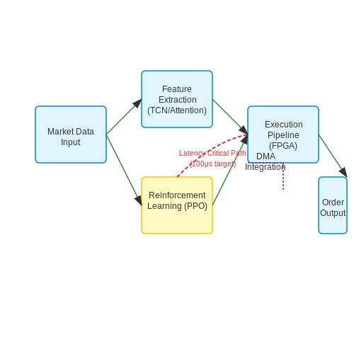
Neural trading agents operate within a high-frequency decision-making framework, where latency and predictive accuracy are critical. The core architecture consists of three modular components:
- Feature Extraction Engine: Processes raw market data (order books, tick data, news sentiment) into low-dimensional embeddings using temporal convolutional networks (TCNs) or attention mechanisms.
- Reinforcement Learning Core: Implements a modified Proximal Policy Optimization (PPO) algorithm with risk-adjusted reward shaping:
where λ controls risk aversion and σ² represents portfolio volatility.
Latency-Optimized Execution
For sub-millisecond decision cycles, trading agents employ:
- Quantized neural networks (8-bit precision) with FPGA acceleration
- Event-driven inference pipelines bypassing traditional batch processing
- Direct market access (DMA) integration through kernel-bypass networking
Market Impact Modeling
Advanced agents incorporate price impact functions during order placement:
where Q is order size, V is market volume, and β ≈ 0.5 based on empirical studies of equity markets.
Adversarial Robustness
To prevent exploitation by counterparties, trading agents implement:
- Generative adversarial networks (GANs) to simulate spoofing attacks during training
- Differential privacy in feature aggregation to obscure trading signals
- Real-time anomaly detection using isolation forests on order flow patterns
Case Study: Crypto Arbitrage Agent
A deployed ETH/BTC arbitrage agent demonstrates:
- Cointegration-based error correction between asset pairs
- Gas price-optimized transaction batching on Ethereum
- Adaptive latency compensation across 17 exchange APIs
Regulatory Constraints
Compliant agents implement:
- Circuit breaker triggers based on VIX-derived volatility thresholds
- Pre-trade risk checks aligned with MiFID II requirements
- Explainability modules generating SHAP values for audit trails
Interactive AI Assistants and Chatbots
Architecture of Neural Conversational Agents
Modern interactive AI assistants rely on transformer-based architectures, such as GPT-4 or PaLM, which employ self-attention mechanisms to process sequential input data. The core computational block is the multi-head attention layer, which computes weighted relationships between tokens in the input sequence. For a sequence of length n, the attention weights A are derived as:
where Q, K, and V are learned query, key, and value matrices, and dk is the dimension of the key vectors. This mechanism allows the model to dynamically focus on relevant context while generating responses.
Real-Time Inference Optimization
To achieve low-latency responses, neural agents employ techniques like:
- Model quantization – Reducing precision from 32-bit floats to 8-bit integers without significant accuracy loss.
- Dynamic batching – Grouping multiple user queries into a single forward pass.
- Cached attention – Reusing computed attention states for repeated dialogue turns.
The inference latency L for a batch size b and sequence length n follows:
where dmodel is the hidden dimension size. Optimizing these parameters enables sub-200ms response times even for billion-parameter models.
Multi-Turn Dialogue Management
Effective chatbots maintain conversation state through:
- Explicit state tracking – Database-backed storage of user preferences and dialogue history.
- Implicit memory – Attention over previous turns stored in key-value caches.
- Reinforcement learning – Fine-tuning with human feedback to optimize for engagement and correctness.
The dialogue policy π selects actions a given state s by maximizing expected reward R:
Evaluation Metrics
Beyond traditional NLP metrics like BLEU, modern systems are evaluated on:
- Coherence – Human-rated logical flow of responses.
- Engagement – Measured by conversation length and user return rate.
- Factual accuracy – Percentage of claims verifiable against knowledge bases.
The F1 score for factual accuracy is computed as:
Case Study: Medical Diagnosis Chatbot
A deployed system at Mayo Clinic uses constrained decoding to ensure all generated medical advice cites peer-reviewed sources. The model first retrieves relevant papers using:
then generates responses conditioned on the top-k documents, reducing hallucinations by 72% compared to base GPT-4.
5. Bias and Fairness in Neural Agents
5.1 Bias and Fairness in Neural Agents
Neural agents, particularly those deployed in real-time reasoning systems, inherit biases from their training data, architectural choices, and optimization objectives. These biases manifest in skewed predictions, discriminatory behavior, or unfair resource allocation, raising ethical and operational concerns. Understanding and mitigating bias requires a multi-faceted approach involving data preprocessing, algorithmic fairness constraints, and post-hoc analysis.
Sources of Bias in Neural Agents
Bias originates from three primary sources:
- Data Bias: Training datasets often underrepresent minority groups or encode historical prejudices. For example, facial recognition systems trained on imbalanced datasets exhibit higher error rates for darker-skinned individuals.
- Algorithmic Bias: Optimization objectives like cross-entropy loss may prioritize majority-class accuracy at the expense of minority groups. Reinforcement learning agents can also develop exploitative strategies if reward functions are misspecified.
- Deployment Bias: Real-world distribution shifts or adversarial inputs can exacerbate biases not present during training. A loan approval agent may unfairly reject applicants from certain ZIP codes if the training data lacked geographic diversity.
Quantifying Fairness
Fairness metrics mathematically formalize disparate impact. Let X be input features, Y the true labels, and A a protected attribute (e.g., gender, race). Common fairness criteria include:
where Ŷ is the model's prediction. These constraints are often mutually exclusive—satisfying one may violate another, as demonstrated by the impossibility theorem of fairness.
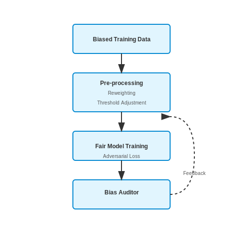
Mitigation Techniques
Pre-processing Methods
Reweighting training samples inversely proportional to their group prevalence balances class distributions. For a dataset with groups Gi, sample weights wi are computed as:
where N is the total samples and k the number of groups.
In-processing Methods
Adversarial debiasing introduces a discriminator network that penalizes the primary model for encoding protected attributes in its latent representations. The loss function becomes:
where λ controls the fairness-accuracy trade-off. Gradient reversal layers ensure the adversary cannot reliably predict A from intermediate features.
Post-processing Methods
Rejection option classification adjusts decision thresholds for different groups. Given a classifier's confidence score s(x), predictions near 0.5 (the uncertainty region) are reassigned based on group-specific error disparities:
Thresholds τ+a and τ-a are optimized to satisfy fairness constraints while minimizing rejections.
Case Study: Fairness in Hiring Agents
A neural agent screening resumes was found to downgrade applications from women for engineering roles. Analysis revealed the training data contained historically biased hiring decisions. The solution combined:
- Reweighting past applications to balance gender representation
- Adding an adversarial loss to remove gender-correlated patterns from learned embeddings
- Post-hoc audit using counterfactual testing (e.g., "Would this resume receive the same score if the gender marker were flipped?")
5.2 Safety and Reliability in Critical Applications
Formal Verification of Neural Agent Decisions
Neural agents operating in safety-critical domains require formal guarantees that their decisions satisfy predefined safety constraints. This is typically achieved through formal verification methods that mathematically prove the absence of hazardous behaviors within specified operational bounds. For a neural network f with inputs x and outputs y, we define a safety property ϕ that must hold for all valid inputs:
Where Xvalid represents the operational design domain. Modern verification approaches employ satisfiability modulo theories (SMT) solvers or mixed-integer linear programming (MILP) to exhaustively check all possible executions. For ReLU-based networks, the verification problem can be formulated as:
If no such x exists, the network is provably safe. Tools like Marabou or NeuralSAT implement these techniques with optimizations for real-time operation.
Runtime Monitoring Architectures
Even with formal verification, runtime monitoring provides an additional safety layer by continuously checking agent outputs against dynamic safety envelopes. A typical monitor implements:
- Predictive safety checking: Projects future states using system dynamics models
- Anomaly detection: Compares observed behavior against expected patterns
- Fallback protocols: Activates when safety thresholds are breached
The monitor's decision function M(y) can be expressed as:
Uncertainty-Aware Decision Making
Neural agents must quantify and act upon epistemic (model) and aleatoric (data) uncertainty. Bayesian neural networks provide principled uncertainty estimates through posterior distributions over weights:
Where D represents training data and w network weights. In practice, Monte Carlo dropout approximates this:
With T forward passes using different dropout masks ŵt. Decisions are then constrained by uncertainty thresholds:
Fault-Tolerant System Design
Critical applications employ redundancy through architectures like:
- N-version programming: Independent implementations voting on outputs
- Watchdog subsystems: Parallel simpler models verifying complex ones
- Heartbeat monitoring: Temporal consistency checks on decision streams
The probability of system failure Pf with n redundant components each having failure probability p follows:
For dissimilar redundancy where failures are uncorrelated.
Case Study: Autonomous Medical Diagnostics
In FDA-cleared AI diagnostic systems, safety measures include:
- Pre-deployment verification on multi-center trial data
- Continuous calibration monitoring against clinician consensus
- Hard-coded decision boundaries for high-risk classifications
Performance is evaluated through metrics like:
Where critical cases represent life-threatening conditions requiring perfect recall.
5.3 Scalability and Deployment Challenges
Computational Bottlenecks in Distributed Neural Agents
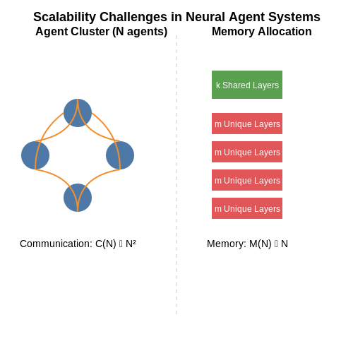
Real-time reasoning with neural agents introduces significant computational bottlenecks when scaling to distributed environments. The primary challenge arises from the need for low-latency synchronization between agents while maintaining high throughput. Consider a multi-agent system where each agent operates as a neural network with parameters θi. The communication overhead for gradient updates in a decentralized setting grows quadratically with the number of agents N:
Here, Li represents the local loss function for agent i, and 𝕀 is an indicator function ensuring agents only communicate with peers. This quadratic scaling makes naive implementations impractical beyond small clusters.
Memory Constraints and Parameter Sharing
Neural agents deployed in resource-constrained environments must balance model complexity with memory limitations. A common approach involves parameter sharing through a centralized critic or attention-based routing. The memory footprint M of an agent system with k shared layers and m unique layers per agent follows:
where d is the hidden dimension. This linear scaling with N becomes problematic when deploying thousands of agents on edge devices with limited RAM. Techniques like gradient checkpointing and dynamic pruning can reduce memory usage by 40-60% in practice.
Latency-Throughput Tradeoffs
Real-time systems require strict latency guarantees while maintaining sufficient throughput. For neural agents processing sequential data, the end-to-end latency τ is bounded by both computational and communication delays:
where tcomp(i) includes both forward pass and local reasoning time, while tcomm(i) covers network synchronization. Parallelization strategies like pipelined execution and speculative reasoning can break this bottleneck, but introduce new challenges in consistency maintenance.
Fault Tolerance in Distributed Deployment
Neural agents operating in real-world environments must handle node failures gracefully. The probability of system failure Pfail in a cluster of N agents with individual failure probability p follows:
This assumes the system fails when ≥2 agents crash. Byzantine fault-tolerant consensus protocols adapted for neural networks, such as federated averaging with robust aggregation, can maintain functionality even with 30-40% malicious or failed nodes.
Dynamic Load Balancing Techniques
Uneven workload distribution across neural agents creates hotspots that degrade performance. Let λi be the arrival rate for agent i and μi its service rate. The load imbalance metric ρ is:
Modern solutions employ reinforcement learning to dynamically adjust agent responsibilities, reducing ρ by 2-3× compared to static allocation in production systems.
Energy Efficiency Considerations
Deploying neural agents on battery-powered devices requires careful energy management. The total power consumption Ptotal combines static and dynamic components:
where α is activity factor, C is switching capacitance, V is voltage, and f is frequency. Techniques like dynamic voltage and frequency scaling (DVFS) adapted for neural agents can achieve 20-35% energy savings while maintaining reasoning quality.
6. Key Research Papers and Surveys
6.1 Key Research Papers and Surveys
- Explainable Goal-driven Agents and Robots - A Comprehensive Review — The KAGR technique used in MAS formulates agent reasoning for specific events as a ... The explanation generation phase is dependent on the behavior of the AI of the agent or robot. The key research directions of this phase are as follows: ... and David W. Aha. 2011. Case-based learning in goal-driven autonomy agents for real-time strategy ...
- Leveraging Reasoning Agents with Chain of Thought (CoT) as Judges in ... — Scalability Concerns : Evaluating many tasks via large models can be computationally expensive, especially if real-time or large-scale throughput is required [16]. 1.3 Introduction to Reasoning Agents as Evaluation Agents Using CoT . To address these challenges, we propose Reasoning Agents ... Ari, et al. The Curious Case of Neural Text ...
- (PDF) RAG-Gym: Optimizing Reasoning and Search Agents ... - ResearchGate — ReSearch explicitly aligns reasoning with query generation, leading to more targeted retrieval and improved answer quality. Template used for history knowledge summarization in Search-o1 and ReSearch.
- [2208.13266] JARVIS: A Neuro-Symbolic Commonsense Reasoning Framework ... — Building a conversational embodied agent to execute real-life tasks has been a long-standing yet quite challenging research goal, as it requires effective human-agent communication, multi-modal understanding, long-range sequential decision making, etc. Traditional symbolic methods have scaling and generalization issues, while end-to-end deep learning models suffer from data scarcity and high ...
- Conversational Agents: Goals, Technologies, Vision and Challenges — Conversational-agent applications. 3. CA's Design Issues. This section describes the different components related to CA design. CA design is divided into four classes: text components for chatbots; CA components related to voice-based virtual agents; physical-related components for goal-oriented CAs or for embodied agents; and task-performance components for goal oriented CAs.
- RAG-Gym: Optimizing Reasoning and Search Agents with Process Supervision — Our key contributions are four-fold: (1) We introduce RAG-Gym, a unified framework for optimizing agentic RAG with process supervision. (2) We propose ReSearch, a novel agent architecture that synergizes answer reasoning and search, achieving state-of-the-art performance over existing baselines. (3) We demonstrate that using trained process re-
- PDF Learning, Reasoning, and Planning with Relational and Temporal Neural ... — vary (orange), relational reasoning layers are fixed at 3. When we have 0 temporal reasoning layers, we predict the sequence label based on the feature of the frame of interest. The purple line shows the performance on temporally warped trajectories when we have the # of relational reasoning layers fixed and vary the # of temporal reasoning layers.
- Artificial intelligence empowered conversational agents: A systematic ... — Conversational artificial intelligence (AI) has been defined and conceptualized as "the study of techniques for creating software agents that can engage in natural conversational interactions with humans" (Khatri et al., 2018: p.41).Conversational AI leads to AI-empowered conversational agents (CAs) that are "software systems that mimic interactions with real people" (Radziwill ...
- (PDF) Advancing Retrieval-Augmented Generation (RAG) Innovations ... — As AI-driven retrieval systems continue to evolve, their integration with reasoning models (e.g., OpenAI o1/o3), Graph Neural Networks (GNNs), Reinforcement Learning (RL), Multi-Agent Systems, and ...
- Relational Reasoning Using Neural Networks: A Survey - ResearchGate — In this paper a comparative review of all relational reasoning-based RN models using deep learning techniques is presented. Automatic evaluation system for e-learning based on emotion recognition.
6.2 Open-Source Implementations and Toolkits
- OpenR: An Open Source Framework for Advanced Reasoning with Large ... — In this technical report, we introduce OpenR, an open-source framework designed to integrate key components for enhancing the reasoning capabilities of large language models (LLMs). OpenR unifies data acquisition, reinforcement learning training (both online and offline), and non-autoregressive decoding into a cohesive software platform. Our goal is to establish an open-source platform and ...
- OpenR : An Open Source Framework for Advanced Reasoning with Large ... — Every contribution is valuable to the community. Thank you for your interest in OpenR! 🥰 We are deeply committed to the open-source community, and we welcome contributions from everyone.Your efforts, whether big or small, help us grow and improve. Contributions aren't limited to code—answering questions, helping others, enhancing our documentation, and sharing the project are equally ...
- NVIDIA Launches Family of Open Reasoning AI Models for Developers and ... — GTC—NVIDIA today announced the open Llama Nemotron family of models with reasoning capabilities, designed to provide developers and enterprises a business-ready foundation for creating advanced AI agents that can work independently or as connected teams to solve complex tasks. Built on Llama models, the NVIDIA Llama Nemotron reasoning family delivers on-demand AI reasoning capabilities.
- Open-RAG: Enhanced Retrieval Augmented Reasoning with Open-Source Large ... — To mitigate this gap, in this paper, we introduce a novel framework, Open-RAG, designed to enhance reasoning capabilities in RAG with open-source LLMs. Our framework transforms an arbitrary dense LLM into a parameter-efficient sparse mixture of experts (MoE) model capable of handling complex reasoning tasks, including both single- and multi ...
- GitHub - theworldofagents/Agentic-Reasoning: free and open OpenAI Deep ... — An open-source framework for deep research and beyond. The core idea is to integrate agentic tools into LLM reasoning. Warning: Still in development. Theoretically runnable, but undergoing rapid updates.
- Open-NARS — Open-NARS is the open source version of the NARS project, a general-purpose AI system, designed in the framework of a reasoning system, which attempts to uniformly explain and reproduce many cognitive facilities, including reasoning, learning, planning, etc., so as to provide a unified theory, model, and system for AI as a whole. The ultimate goal of this research is to build a thinking machine.
- Stable-Baselines3: Reliable Reinforcement Learning Implementations — Stable-Baselines3 provides open-source implementations of deep reinforcement learning (RL) algorithms in Python. The implementations have been benchmarked against reference codebases, and automated unit tests cover 95% of the code. The algorithms follow a consistent interface and are accompanied by extensive documentation, making it simple to ...
- DeepSeek: Revolutionizing AI with Open-Source Reasoning Models ... — DeepSeek-R1's competitive edge lies in its open-source approach, cost efficiency, and adaptability to niche reasoning domains. While OpenAI and Google models lead in multimodal applications ...
- Open AI Strawberry — The Role of Decision Trees and RL in ... - Medium — Understanding the reasoning process of LLMs remains a challenge due to the opaque nature of neural networks. Alignment: Ensuring that the model's reasoning aligns with human values and ...
- Learning to Walk with Dual Agents for Knowledge Graph Reasoning — This paper proposed a dual-agent based reinforcement learning approach to tackle the KG reasoning problem. Existing RL-based learning to walk methods rely solely on one entity-level agent to explore large KGs, which works well on finding short reasoning paths, but usually succumb to longer patterns ...
6.3 Recommended Books and Online Courses
- Conversational Agents: Goals, Technologies, Vision and Challenges — They group the conversational agents into three categories: question-answering agents, task-oriented dialogue agents, and chatbots. For each category, they present a review of state-of-the-art neural approaches, draw the connection between neural and traditional approaches, and discuss the progress that has been made and challenges still being ...
- PDF Bayesian Reasoning and Machine Learning — The book begins with the basic concepts of graphical models and inference. For the independent reader Chapters 1, 2, 3, 4, 5, 9, 10, 13, 14, 15, 16, 17, 21 and 23 would form a good introduction to probabilistic reasoning, modelling and machine learning.
- Neural Networks and Learning Machines - Pearson — For graduate-level neural network courses offered in the departments of Computer Engineering, Electrical Engineering, and Computer Science. Renowned for its thoroughness and readability, this well-organized and completely up-to-date text remains the most comprehensive treatment of neural networks from an engineering perspective.
- PDF Artificial Intelligence - MRCE — "Poole and Mackworth'sArtificial Intelligence: Foundations of Computational Agents 3eis a tour de force. This is a comprehensive and clearly written text that takes the reader through core concepts in symbolic AI and machine learning, providing pathways for broad introductory undergraduate courses, or focused graduate courses.
- Non-axiomatic logic [electronic resource] : a model of intelligent ... — Reasoning processes according to this logic covers cognitive functions like learning, planning, decision making, problem solving, etc.This book is written for researchers and students in Artificial Intelligence and Cognitive Science, and can be used as a textbook for courses at graduate level, or upper-level undergraduate, on Non-Axiomatic ...
- PDF Artificial Intelligence: Foundations of Computational Agents — "This revised and extended edition of Artificial Intelligence: Foundations of Computational Agents should become the standard text of AI education. Computer science students will find in this volume a broad and uniquely coherent perspective on many com-putational models of learning, reasoning, and decision-making.
- PDF Natural Language Processing - University of California, San Diego — The book is targeted at computer scientists, who are assumed to have taken introductory courses on the analysis of algorithms and complexity theory. In particular, you should be familiar with asymptotic analysis of the time and memory costs of algorithms, and with the basics of dynamic programming.
- Emergent analogical reasoning in large language models — Webb et al. show that new artificial intelligence language models, such as Generative Pre-trained Transformer 3, are able to solve analogical reasoning problems at a human-like level of performance.
- Full Table of Contents for AI: A Modern Approach — Part I: Artificial Intelligence Chapter 1 Introduction ... 1 What Is AI? ... 1 1.1.1 Acting humanly: The Turing test approach ... 2 1.1.2 Thinking humanly: The cognitive modeling approach ... 2 1.1.3 Thinking rationally: The ``laws of thought'' approach ... 3 1.1.4 Acting rationally: The rational agent approach ... 3 1.1.5 Beneficial machines ... 4 1.2 The Foundations of Artificial ...
- (PDF) Latest Advances in Agentic AI Architectures, Frameworks ... — PDF | The rapid advancements in Agentic Artificial Intelligence (Agentic AI) have significantly reshaped the landscape of autonomous systems, achieving... | Find, read and cite all the research ...