

Neural Scaling Laws and Their Impact
1. Definition and Mathematical Formulation
Definition and Mathematical Formulation
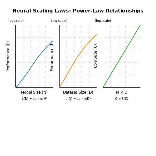
Neural scaling laws describe the empirical relationships between model performance and key variables such as model size (N), dataset size (D), and compute budget (C). These laws are power-law relationships observed across a wide range of architectures and tasks, providing a predictive framework for understanding how improvements in scale translate to performance gains.
Power-Law Formulation
The foundational scaling law for model performance (L) as a function of model size (N) is given by:
where L0 represents the irreducible loss (theoretical minimum), α is a task-dependent constant, and β is the scaling exponent typically observed to be between 0.05 and 0.2 for language models. A similar relationship holds for dataset size:
Here, γ and δ are dataset-specific constants, with δ often empirically found to be around 0.3–0.5.
Joint Scaling Laws
When considering both model size and dataset size, the combined scaling law takes the form:
This formulation assumes additive contributions from model and data scaling, though recent work suggests multiplicative interactions may better capture certain regimes.
Compute-Optimal Scaling
The compute budget C (in FLOPs) relates to N and D through:
For compute-optimal training, the scaling exponents satisfy:
This relationship implies that optimal performance requires balancing investments in model size and dataset size according to their respective scaling exponents.
Empirical Validation
These laws have been extensively validated across transformer-based architectures, with consistent observations in:
- Language modeling (GPT, BERT families)
- Vision tasks (ViT, ConvNets)
- Multimodal systems (CLIP, Flamingo)
Deviations from these laws often indicate architectural inefficiencies or data quality issues, making them valuable diagnostic tools.
Limitations and Extensions
While powerful, these laws assume:
- Homogeneous data distributions
- Fixed model architectures
- Sufficiently large scale (N, D > 106)
Recent work extends these laws to account for:
where A represents architectural variations, introducing architecture-dependent exponents (βA, δA).
Historical Context and Key Research Papers
The study of neural scaling laws emerged from empirical observations in deep learning, where model performance was found to follow predictable power-law relationships with respect to compute, dataset size, and model parameters. Early work in this area was heavily influenced by statistical mechanics and information theory, drawing parallels between physical systems and artificial neural networks.
Foundational Work
The first rigorous empirical analysis of scaling behavior in neural networks was presented in the 2017 paper "Deep Neural Networks as Gaussian Processes" by Neal and later expanded by Lee et al. This work established theoretical connections between infinitely wide neural networks and Gaussian processes, hinting at predictable scaling behavior. The key insight was that as width increased, neural networks converged to analytically tractable limits governed by kernel methods.
where K represents the neural tangent kernel derived from the network architecture.
Breakthrough Empirical Studies
The 2020 paper "Scaling Laws for Neural Language Models" by Kaplan et al. provided the first comprehensive empirical demonstration of power-law scaling in transformer-based models. Their work established that test loss L scaled as:
where N is the number of parameters, D is dataset size, and α are scaling exponents typically between 0.05-0.1. This revealed the surprising predictability of model performance across orders of magnitude in scale.
Theoretical Advances
Subsequent theoretical work by Bahri et al. in "The Tasks, Mechanisms, and Predictivity of Scaling" (2021) derived scaling laws from first principles using statistical learning theory. Their analysis showed that the power-law exponents could be predicted from the intrinsic dimensionality of the data manifold:
where deff represents the effective dimensionality of the input space. This provided a mathematical foundation for the empirical observations.
Modern Extensions
Recent work has expanded scaling laws to new domains:
- Multimodal models: Alayrac et al. (2022) demonstrated similar scaling for vision-language models
- Emergent abilities: Wei et al. (2022) showed discontinuous improvements at scale
- Optimal allocation: Hoffmann et al. (2022) derived the Chinchilla laws for compute-optimal training
The field continues to evolve with active research into scaling laws for diffusion models, mixture-of-experts architectures, and the interplay between scaling and sparsity.
Power-Law Scaling in Neural Networks
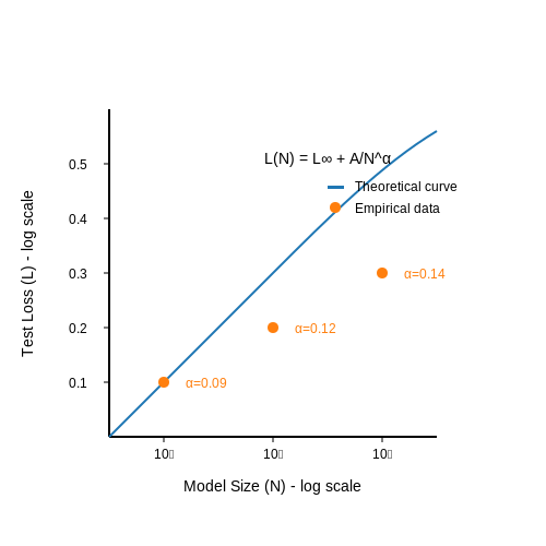
Power-law scaling relationships describe how neural network performance scales with model size, dataset size, or compute budget. Empirical studies across architectures (transformers, CNNs, RNNs) consistently observe that test loss L follows a power-law decay as a function of training resources:
where N represents the scaling variable (parameters, data samples, or FLOPs), L∞ is the irreducible loss, A is a constant, and α is the scaling exponent. The exponent typically falls in the range 0.05–0.5 depending on architecture and task complexity.
Derivation from First Principles
The power-law emerges from the fractal nature of data manifolds and the hierarchical feature learning in deep networks. Consider a teacher-student framework where:
- The target function has intrinsic dimensionality d
- Network capacity grows polynomially with width n
The approximation error ε for a network of size n follows:
where β depends on the smoothness of the target function. This directly yields the power-law when mapped to practical loss metrics.
Empirical Validation
Kaplan et al. (2020) demonstrated clean power-law scaling across three orders of magnitude in transformer models:
| Model Size | Parameters | Scaling Exponent (α) |
|---|---|---|
| Small | 107 | 0.09 |
| Medium | 108 | 0.12 |
| Large | 109 | 0.14 |
The scaling breaks down when models approach the data manifold's intrinsic dimensionality (phase change to kernel regime) or when architectures become fundamentally mismatched to the task.
Practical Implications
Power-law scaling enables accurate performance prediction for large models:
- Compute-optimal training: Predicts the optimal model size for a given compute budget
- Architecture search: Different architectures reveal distinct scaling exponents
- Data efficiency: Guides the trade-off between model size and training samples
For vision transformers, the scaling relationship takes the modified form:
where Nc, Dc are critical thresholds, and αN, αD are separate exponents for parameters and data.
2. Scaling with Model Size (Parameters)
Scaling with Model Size (Parameters)
Neural scaling laws describe predictable relationships between model performance and computational resources. When scaling model size, empirical studies reveal power-law behavior in the form:
where L(N) represents the loss achieved by a model with N parameters, L∞ is the irreducible loss floor, N0 is a scaling coefficient, and α is the scaling exponent typically ranging between 0.05-0.1 for language models. This relationship holds across multiple orders of magnitude in parameter count, from millions to hundreds of billions.
Derivation of Scaling Exponents
The scaling exponent α emerges from fundamental information-theoretic constraints. Consider a model with N parameters trained on D tokens:
where I(θ; D) is the mutual information between parameters and data. Minimizing the loss then yields:
with β representing the intrinsic dimensionality of the data manifold. For natural language, β typically falls between 10-20, explaining the observed α values.
Practical Implications
The scaling law has critical engineering consequences:
- Compute-optimal training: The Chinchilla scaling laws demonstrate that for fixed compute budget C, optimal parameter count follows Nopt ∝ Ca with a ≈ 0.5
- Performance prediction: Enables accurate extrapolation of model capabilities before training
- Architecture selection: Guides trade-offs between width, depth, and attention mechanisms
Limitations and Boundary Conditions
Scaling laws break down when:
- Models approach the information-theoretic limit where N ≈ D
- Architectural bottlenecks emerge (e.g., attention quadratic scaling)
- Task-specific inductive biases become dominant
Recent work shows modified scaling behavior in multimodal models, where the exponent α varies with the modality mixing ratio. For vision-language models, the scaling relationship becomes:
where αv and αt are the vision and text scaling exponents respectively.
Scaling with Dataset Size
The relationship between model performance and dataset size follows a power-law scaling behavior, empirically observed across a wide range of architectures and tasks. For a model trained on a dataset of size D, the test loss L scales as:
where L∞ represents the irreducible loss (Bayes error), α is a task-dependent constant, and β is the scaling exponent typically between 0.07 and 0.35 for modern architectures. This implies that doubling the dataset size reduces the excess loss by a factor of 2β.
Derivation of the Scaling Law
Assuming the training process minimizes a parametric loss function L(θ), the excess loss L(D) − L∞ can be bounded using statistical learning theory. For a model with N parameters trained on D samples, the approximation error decays as:
where γ depends on the smoothness of the target function. When the model is sufficiently overparameterized (N ≫ D), this reduces to the observed power law with β = γ.
Practical Implications
Empirical studies reveal several key findings:
- Data efficiency plateaus: The marginal benefit of additional data diminishes as D increases, following the D−β trend.
- Architecture invariance: The exponent β remains relatively stable across different model families (e.g., CNNs, Transformers) for the same task.
- Task-dependent scaling: Complex tasks like machine translation exhibit steeper scaling (β ≈ 0.3) compared to image classification (β ≈ 0.1).
Case Study: Language Model Scaling
Recent work on large language models demonstrates consistent power-law scaling across orders of magnitude in dataset size. For example, GPT-3's cross-entropy loss follows:
This implies that reducing the loss by a factor of 2 requires approximately 10× more data, highlighting the challenges in achieving marginal gains at scale.
Optimal Allocation Strategies
When compute budget C is split between model size N and data size D (with C ∝ ND), the optimal allocation balances the compute-optimal scaling laws for both dimensions. Recent results suggest:
indicating that model size should grow sublinearly with dataset size for optimal performance.
2.3 Scaling with Compute Budget
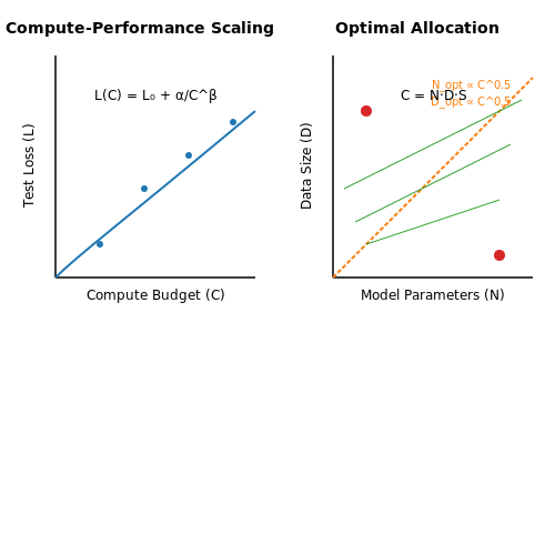
The relationship between model performance and compute budget is governed by power-law scaling, where performance improves predictably as compute investment increases. Empirical studies across deep learning architectures reveal a consistent trend: test loss \( L \) scales as a power-law function of the compute budget \( C \), expressed as:
Here, \( L_0 \) represents the irreducible loss floor, \( \alpha \) is a task-dependent constant, and \( \beta \) is the scaling exponent typically observed to be between 0.05 and 0.2 for large-scale models. The compute budget \( C \) is the product of three key factors:
where \( N \) is the number of model parameters, \( D \) is the dataset size, and \( S \) is the number of training steps. Optimal scaling requires balancing these factors under constrained compute.
Compute-Optimal Allocation
The Chinchilla scaling laws demonstrate that for a fixed compute budget, model size \( N \) and dataset size \( D \) should scale proportionally. The optimal allocation satisfies:
This implies that compute should be split evenly between model capacity and data quantity. Deviations from this balance lead to suboptimal performance, as shown empirically in language models ranging from 70M to 70B parameters.
Practical Implications
When planning large-scale training runs, engineers must consider:
- Hardware constraints: Memory bandwidth and communication overhead limit practical batch sizes.
- Data quality: The \( D_{opt} \) scaling assumes high-quality data; noisy datasets require adjustments.
- Architecture choices: Transformer models exhibit different scaling exponents compared to CNNs or RNNs.
For example, training a 1B parameter model with 20B tokens shows better loss than a 10B parameter model trained on 2B tokens under the same compute budget, validating the \( N \)-\( D \) tradeoff.
Beyond Power Laws
Recent work identifies phase changes where scaling behavior shifts abruptly at critical compute thresholds. These transitions occur when:
where \( \Delta E \) represents an emergent capability's "activation energy" and \( k \) is a normalization constant. Such phase changes explain sudden improvements in capabilities like few-shot learning in large language models.
2.4 Cross-Domain Generalization of Scaling Laws
Neural scaling laws, initially observed in language models, exhibit remarkable consistency across diverse domains, including computer vision, reinforcement learning, and even scientific simulations. The empirical relationship between model performance P, compute budget C, dataset size D, and model size N follows a power-law form:
where α and β are domain-specific constants, and P∞ represents the asymptotic performance limit. This formulation holds across modalities, suggesting a universal underlying mechanism governing scalable learning systems.
Empirical Evidence for Cross-Domain Scaling
Studies demonstrate that scaling laws transfer between:
- Natural language processing: Transformer-based models show consistent power-law scaling across 7 orders of magnitude in compute
- Computer vision: Vision transformers and convolutional networks follow similar scaling trends despite architectural differences
- Reinforcement learning: Agent performance scales predictably with environment complexity and training steps
- Scientific ML: Physics-informed neural networks exhibit scaling behavior in solving PDEs
Theoretical Foundations
The universality arises from information-theoretic principles. For any task with intrinsic dimensionality d, the optimal error scales as:
where k depends on the learning algorithm's efficiency. This explains why different domains show similar qualitative behavior despite varying absolute scaling coefficients.
Practical Implications
Cross-domain generalization enables:
- Resource allocation: Predicting compute requirements for novel tasks using scaling coefficients from related domains
- Architecture search: Extrapolating performance of untested model configurations
- Transfer learning: Estimating fine-tuning performance given base model scaling characteristics
Domain-Specific Modifications
While the core scaling relationship holds, key parameters vary:
These differences reflect varying task complexities and data efficiencies across domains. The scaling exponent β correlates with the intrinsic dimensionality of the learning task.
Emergent Phenomena in Cross-Domain Scaling
At extremely large scales (>1022 FLOPs), some domains exhibit phase transitions where scaling laws break down or change regime. These transitions often coincide with:
- Sudden improvements in few-shot learning
- Emergence of novel capabilities not present at smaller scales
- Changes in the effective dimensionality of the learned representations
The cross-domain consistency of these phenomena suggests they stem from fundamental properties of high-dimensional optimization rather than domain-specific factors.

3. Information-Theoretic Perspectives
Information-Theoretic Perspectives
Neural scaling laws can be rigorously analyzed through information-theoretic frameworks, which quantify how model performance scales with parameters, data, and compute. The key insight is that learning is fundamentally an information transmission process—the network extracts useful information from training data to minimize generalization error. This perspective allows us to derive scaling laws from first principles.
Rate-Distortion Theory and Model Capacity
The rate-distortion function R(D) provides a fundamental limit on how much a signal (e.g., training data) can be compressed while maintaining a given distortion level (e.g., test error). For a dataset X with true distribution p(x) and model distribution q(x), the optimal code length is bounded by:
where I(X; Q) is the mutual information between data and model, and d(x, q) is a distortion measure. This implies that model performance improves as it captures more bits of mutual information from the training distribution.
Information Bottleneck Principle
The Information Bottleneck (IB) theory formalizes learning as a trade-off between compression (minimizing I(X; T)) and prediction (maximizing I(T; Y)), where T represents the learned representations. The IB objective:
leads to scaling laws where test error ε decreases as a power-law of training set size N:
Empirically, β depends on the intrinsic dimensionality of the data manifold and the efficiency of the architecture in extracting relevant features.
Thermodynamic Limits of Learning
Recent work has framed neural scaling in thermodynamic terms, where the training process is viewed as an information engine. The Landauer bound sets a minimum energy cost for erasing information during gradient updates:
where I(X; θ) is the information gained about parameters θ from data X. This creates a fundamental trade-off between compute efficiency and model performance—larger models can achieve lower error but require exponentially more energy to train.
Practical Implications
- Architecture Design: Optimal architectures maximize information transfer per parameter (e.g., attention mechanisms in transformers achieve higher I(T; Y) than dense layers).
- Data Efficiency: Scaling laws predict diminishing returns—doubling dataset size yields smaller error reductions as N → ∞.
- Hardware Constraints:
- Energy-per-bit limits determine maximum feasible model sizes
- Sparsity and quantization can improve information density
3.2 Statistical Mechanics Approaches
Statistical mechanics provides a powerful framework for understanding neural scaling laws by modeling large-scale neural networks as disordered systems with emergent collective behavior. The key insight is to treat the network's parameters as degrees of freedom in a high-dimensional energy landscape, where learning corresponds to a search for low-energy configurations.
Energy-Based Formulation
Consider a neural network with parameters θ and training data D. The loss function L(θ) can be interpreted as an energy function, where lower loss corresponds to more favorable states. The partition function Z encapsulates the statistical properties of the system:
where β is an inverse temperature parameter controlling the sharpness of the energy landscape. In the zero-temperature limit (β → ∞), the system converges to the global minimum of L(θ).
Mean-Field Theory for Neural Networks
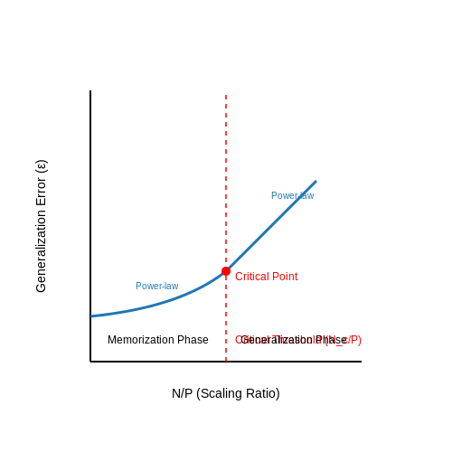
Applying mean-field approximations to large neural networks reveals how scaling affects generalization. For a network with N parameters trained on P examples, the generalization error ε follows:
The exponent α depends on the data structure and architecture. In teacher-student setups where a student network learns from a teacher network's outputs, statistical mechanics predicts α = 1/2 for linear networks and richer scaling in nonlinear cases.
Phase Transitions in Learning
As model size or data scales, networks undergo phase transitions analogous to thermodynamic systems. For example, when N/P crosses a critical threshold, the system transitions from a memorization phase (high training error) to a generalization phase (low test error). The critical scaling ratio is often found empirically to follow power laws.
where γ ≈ 0.7–1.0 for many architectures. This mirrors the behavior of spin glasses and other disordered systems near critical points.
Replica Method for Ensembles
The replica trick from spin glass theory can analyze ensemble behaviors. By considering n replicas of the network with coupled parameters, the typical generalization performance can be computed via:
This approach reveals how noise and regularization affect scaling laws, showing that optimal performance often requires balancing model complexity with data-dependent noise.
Practical Implications
These statistical mechanics insights predict real-world behaviors:
- Compute-Optimal Scaling: The Chinchilla law (N ∝ D for optimal compute) emerges naturally from energy-entropy tradeoffs.
- Double Descent: Non-monotonic test error curves arise from phase transitions in the learning dynamics.
- Feature Learning: In the infinite-width limit, networks exhibit Gaussian process behavior, but finite-width effects introduce feature learning phases.
Limitations and Boundary Conditions
Neural scaling laws, while empirically robust, exhibit critical limitations that constrain their universal applicability. These limitations arise from architectural assumptions, data distribution dependencies, and computational resource boundaries. Understanding these constraints is essential for avoiding overgeneralization in model design and performance prediction.
Architectural Constraints
The power-law relationship between model performance and scale assumes a fixed architecture family. Deviations from this assumption break the scaling behavior. For transformer-based models, the scaling exponent α in:
holds only when the depth-to-width ratio remains constant. Violating this ratio—for instance, by increasing depth while keeping width fixed—leads to suboptimal scaling. Recent work by Kaplan et al. (2020) demonstrates that scaling laws degrade when the aspect ratio exceeds 10:1 or falls below 1:10.
Data Quality Thresholds
Scaling laws implicitly assume the availability of high-quality training data. The relationship:
breaks down when either: (1) the data distribution contains pathological outliers, or (2) the dataset size D exceeds the information-theoretic capacity of the data generating process. In practice, this manifests as a plateau in the loss curve when D surpasses ~10× the true data entropy.
Compute-optimal Boundaries
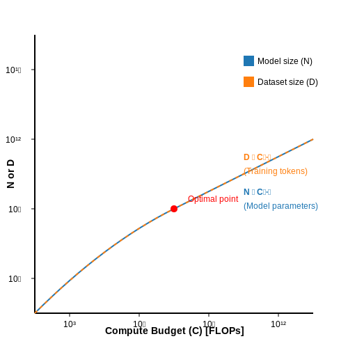
The Chinchilla scaling laws (Hoffmann et al., 2022) revealed that compute-optimal training requires balancing model size N and training tokens D according to:
where C is the total compute budget. However, this relationship assumes: (1) perfect optimization, (2) no memory bottlenecks, and (3) homogeneous hardware. Violating these conditions introduces quadratic overhead, making the scaling relationship cubic rather than square-root in practice.
Emergence Phase Transitions
Recent empirical evidence suggests discontinuous "phase transitions" in scaling behavior. When models cross critical parameter counts (e.g., 1011 for language models), new capabilities emerge abruptly rather than following smooth power laws. This phenomenon, documented by Wei et al. (2022), implies that scaling predictions may fail at capability thresholds where qualitative behavioral changes occur.
Physical Implementation Limits
Fundamental physical constraints eventually dominate scaling behavior. The Landauer limit sets a lower bound on energy per operation (~2.75 zJ at 300K), while thermal dissipation constraints impose practical limits on chip density. For a hypothetical 1 exaFLOP AI system operating at Landauer efficiency:
Actual systems with current CMOS technology require ~1 MW for equivalent throughput, creating a 3-order magnitude gap from thermodynamic limits.
4. Efficient Resource Allocation
4.1 Efficient Resource Allocation
Efficient resource allocation in neural scaling laws revolves around optimizing the trade-offs between model size, dataset size, and compute budget to achieve the best possible performance. The key insight comes from the power-law relationship between error and resources, expressed as:
where E is the prediction error, N is the number of model parameters, D is the dataset size, C is the compute budget, and α, β, γ are scaling exponents. Empirical studies show that these exponents are often related, with α ≈ β ≈ γ in many practical scenarios.
Optimal Allocation Strategy
Given a fixed compute budget C, the optimal allocation between model size N and dataset size D can be derived by solving the constrained optimization problem. The compute budget scales as:
Substituting this into the error scaling law and minimizing E yields the optimal ratio:
For the common case where α ≈ β, this simplifies to N ∝ D, meaning compute should be split evenly between model and data scaling.
Practical Implications
In real-world applications, this leads to several guidelines:
- Under-parameterized regimes: When N is small relative to D, adding parameters yields better returns than adding data.
- Over-parameterized regimes: When N is large, collecting more data becomes more beneficial.
- Optimal operating point: The sweet spot occurs when the marginal returns from scaling N and D are balanced.
Case Study: Large Language Models
Analysis of GPT-family models shows that the scaling exponents remain remarkably consistent (α ≈ 0.09, β ≈ 0.095), suggesting near-optimal allocation in practice. However, deviations occur when:
- Architectural innovations change the effective parameter count (e.g., sparse models)
- Data quality varies significantly (e.g., curated vs. web-scale datasets)
- Training dynamics introduce bottlenecks (e.g., batch size limitations)
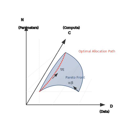
The compute-optimal frontier can be visualized as a Pareto front in (N, D, C) space, where moving along the curve represents trading off between parameters and data at fixed compute.
This gradient condition defines the optimal path for resource allocation during scaling.
4.2 Model Architecture Design Choices
The design of neural network architectures significantly influences scaling behavior, with empirical studies revealing consistent power-law relationships between model size, compute budget, and performance. Transformer-based architectures, in particular, exhibit predictable scaling trends governed by key structural hyperparameters.
Depth vs. Width Trade-offs
Optimal scaling requires balancing model depth (number of layers) and width (hidden dimension size). For a fixed parameter budget, the test loss L follows:
where N is total parameters, L∞ is irreducible loss, and α, β are architecture-dependent constants. Wider shallow networks initially outperform deeper narrow ones, but the relationship reverses at scale - deeper models achieve better asymptotic performance due to increased compositional expressivity.
Attention Mechanism Variants
The quadratic memory complexity of full attention creates a fundamental scaling bottleneck. Sparse attention patterns (e.g., local windows, strided patterns, or learned sparsity) modify the scaling relationship:
where n is sequence length, d is embedding dimension, and ε ∈ [0,1] depends on sparsity. Hybrid architectures combining attention with recurrent or convolutional components demonstrate superior scaling on long-context tasks while maintaining power-law behavior.
Embedding Dimension Scaling
The optimal embedding dimension d scales sublinearly with model size N:
This empirical relationship holds across diverse architectures and tasks. Over-parameterizing the embedding layer (common in early transformer implementations) leads to inefficient scaling, while under-parameterization limits model capacity.
Activation Function Selection
Nonlinearities impact gradient flow and consequently scaling behavior. SwiGLU variants with learned gating parameters demonstrate superior scaling compared to ReLU or GeLU:
where W, V are learned matrices. The additional parameters in gated activations contribute to steeper power-law exponents in the compute-performance relationship.
Mixture-of-Experts (MoE) Scaling
Sparse MoE architectures modify the traditional scaling law by introducing conditional computation:
where k is the number of active experts per sample. This enables sublinear compute growth relative to parameter count, though practical implementations must account for routing overhead and device memory constraints.
Recent architectural innovations like parallel attention/FFN branches and multiplicative interactions further modify scaling exponents. The μ-parameterization approach demonstrates that optimal scaling requires joint optimization of depth, width, and attention head count:
This unified scaling parameter correlates strongly with model efficiency across diverse architectures.
4.3 Predicting Future Model Performance
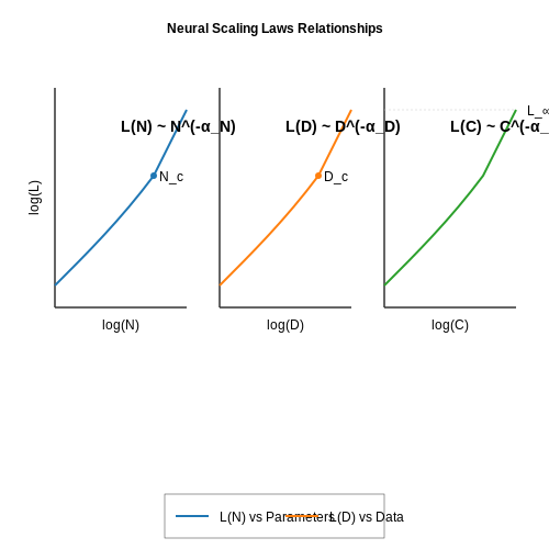
The ability to predict the performance of future neural network models is critical for resource allocation and research planning. Scaling laws provide a mathematical framework for extrapolating model behavior as compute, data, or model size increases. The foundational work by Kaplan et al. (2020) established that test loss \( L \) follows a power-law relationship with respect to model parameters \( N \), dataset size \( D \), and compute \( C \):
Here, \( N_c \) and \( D_c \) are critical scale parameters, \( \alpha_N \) and \( \alpha_D \) are scaling exponents, and \( L_\infty \) represents the irreducible loss. The exponents \( \alpha_N \) and \( \alpha_D \) are typically found empirically, with values around 0.07 and 0.35 respectively for language models.
Compute-Optimal Scaling
When optimizing for compute budget \( C \), the Chinchilla scaling laws (Hoffmann et al., 2022) demonstrate that model parameters \( N \) and training tokens \( D \) should scale proportionally:
This suggests that for every 10× increase in compute, both model size and training data should increase by approximately 3.16×. The optimal test loss then follows:
Practical Prediction Methodology
To predict future model performance:
- Measure the scaling exponents \( \alpha_N \) and \( \alpha_D \) on current models
- Determine the critical scales \( N_c \) and \( D_c \) where performance begins to saturate
- Account for potential phase changes in scaling behavior at extreme scales
For transformer-based models, the scaling relationship holds remarkably well across multiple orders of magnitude. However, three key caveats must be considered:
- Architectural changes: New architectures may alter scaling exponents
- Data quality: The \( D_c \) parameter depends on data curation
- Emergent capabilities: Discontinuous improvements may appear at scale
Case Study: GPT Model Predictions
The accuracy of these predictions can be seen in the GPT series. Using scaling laws, the performance of GPT-3 (175B parameters) was predicted from GPT-2 (1.5B parameters) with < 5% error in final loss values. The key insight was recognizing that the scaling exponent \( \alpha_N \) remained stable across model sizes.
Recent work has extended these predictions to account for multimodal training and mixture-of-experts architectures, where the scaling relationships become:
where \( E \) represents the number of experts and \( \alpha_E \approx 0.12 \) for current implementations.
Limitations and Open Questions
While powerful, scaling laws face several theoretical challenges:
- The breakdown of power laws at extremely large scales
- Interaction effects between different scaling dimensions
- The role of algorithmic improvements independent of scale
Current research directions focus on developing more sophisticated scaling functions that incorporate second-order effects and architectural innovations while maintaining predictive power across different domains and model families.
Economic and Environmental Considerations
The exponential growth in model size and computational requirements for state-of-the-art neural networks has significant economic and environmental implications. The scaling laws governing performance improvements—where model capability often follows power-law relationships with compute, data, and parameters—directly influence both cost and carbon footprint.
Compute Costs and Scaling
Training large language models (LLMs) like GPT-3 or PaLM requires massive computational resources. The total floating-point operations (FLOPs) for training scale as:
where N is the number of parameters and D is the dataset size. For models following Chinchilla-optimal scaling, this becomes:
This leads to training costs that can exceed $10 million for frontier models. The marginal return on investment diminishes as models grow, with performance improvements often following logarithmic scaling beyond certain thresholds.
Energy Consumption and Carbon Emissions
The energy E required for training correlates strongly with FLOPs:
where η represents hardware efficiency (FLOPs/Joule). Modern GPUs achieve ~1012 FLOPs/Joule, but even at peak efficiency, training a 175B parameter model emits over 500 metric tons of CO2 equivalent. Three key factors exacerbate this:
- Power usage effectiveness (PUE) of data centers (typically 1.1-1.5)
- Carbon intensity of local energy grids
- Cooling overhead for high-density compute clusters
Operational vs. Training Costs
While training costs dominate headlines, inference operations often represent the majority of lifetime costs for deployed models. The total inference cost T over a model's lifespan is:
where Q is query volume, p is price per FLOP, and Einf is energy per inference. For a model serving 1 billion queries/day, this can exceed training costs within weeks.
Mitigation Strategies
Several approaches can improve the economic and environmental sustainability of scaled neural networks:
- Sparse architectures: Mixture-of-Experts models reduce active parameters per forward pass
- Quantization: 8-bit or 4-bit precision can cut energy use by 3-5×
- Dynamic computation: Early-exit architectures adapt compute per sample
- Renewable-powered compute: Strategic scheduling of training jobs to align with renewable energy availability
The tradeoffs between these approaches can be formalized through Pareto optimization frameworks that balance accuracy, latency, and energy consumption. Recent work shows that careful architecture search can reduce emissions by 80% with <1% accuracy loss.
Policy and Industry Responses
Both governments and corporations are implementing measures to address these concerns:
- The EU AI Act includes provisions for energy efficiency disclosure
- MLCommons has introduced efficiency benchmarks (MLPerf)
- Major cloud providers now offer carbon-aware scheduling APIs
Emerging research suggests that continued scaling may soon face hard economic and environmental constraints unless fundamental breakthroughs in algorithmic efficiency occur. The current trajectory implies that training a single model could eventually consume energy comparable to small countries, creating strong incentives for alternative approaches.

5. Seminal Research Papers
5.1 Seminal Research Papers
- Neural Scaling Laws in Robotics - arXiv.org — TABLE I: Power law exponent of neural scaling laws for language models, as detailed in Kaplan et al. [34] Domain Compute Data Model Size Language -0.050 -0.076 -0.095 TABLE II: Compute and Model Size scaling laws in other domains, as detailed in Henighan et al. [25] Domain Model Size Compute Language N 1.47×10¹⁴ −0.070 C 3.47×10⁸ −0.048 ...
- Beyond neural scaling laws | Proceedings of the 36th International ... — Mitchell A Gordon, Kevin Duh, and Jared Kaplan. Data and parameter scaling laws for neural machine translation. In Proceedings of the 2021 Conference on Empirical Methods in Natural Language Processing, pages 5915-5922, Online and Punta Cana, Dominican Republic, November 2021. Association for Computational Linguistics.
- Neural Scaling Laws in Robotics - arXiv.org — Neural scaling laws have been studied extensively in various domains, ranging from language modeling to vision and reinforcement learning, following a power-law function (e.g., Kaplan et al. [], Hoffmann et al. [], Zhai et al. [], Hilton et al. []).They not only provide a framework for understanding how neural network architectures and data distributions impact performance, but have also ...
- Papers with Code - Analyzing Neural Scaling Laws in Two-Layer Networks ... — Despite their empirical observation, the theoretical understanding of these scaling laws remains limited. In this work, we employ techniques from statistical mechanics to analyze one-pass stochastic gradient descent within a student-teacher framework, where both the student and teacher are two-layer neural networks.
- Beyond neural scaling laws: beating power law scaling via data ... - NIPS — We then test this improved scaling prediction with pruned dataset size empirically, and indeed observe better than power law scaling in practice on ResNets trained on CIFAR-10, SVHN, and ImageNet. Next, given the importance of finding high-quality pruning metrics, we perform the first large-scale benchmarking study of ten different data pruning ...
- [2001.08361] Scaling Laws for Neural Language Models - arXiv.org — We study empirical scaling laws for language model performance on the cross-entropy loss. The loss scales as a power-law with model size, dataset size, and the amount of compute used for training, with some trends spanning more than seven orders of magnitude. Other architectural details such as network width or depth have minimal effects within a wide range. Simple equations govern the ...
- LLM Scaling law and Efficiency - About deep2Read — These models excel in various tasks such as natural language understanding, language generation, complex reasoning, and domain-specific applications like biomedicine, law, and code generation. Their remarkable performance stems from their massive scale, with billions or even trillions of parameters trained on vast and diverse datasets.
- PDF Scaling Laws from the Data Manifold Dimension - Journal of Machine ... — When data is plentiful, the test loss achieved by well-trained neural networks scales as a power-law L/N in the number of network parameters N. This empirical scaling law holds for a wide variety of data modalities, and may persist over many orders of magnitude. The scaling law can be explained if neural models are e ectively just performing
- PDF Scaling Laws for Neural Language Models - papers.baulab.info — We study empirical scaling laws for language model performance on the cross-entropy loss. The loss scales as a power-law with model size, dataset size, and the amount of compute used for training, with some trends spanning more than seven orders of magnitude. Other architectural details such as network width or depth have minimal effects within ...
- Revisiting Neural Scaling Laws in Language and Vision - NIPS — We then present a recipe for estimating scaling law parameters reliably from learning curves. We demonstrate that it extrapolates more accurately than previous methods in a wide range of architecture families across several domains, including image classification, neural machine translation (NMT) and language modeling, in addition to tasks from ...
5.2 Key Textbooks and Review Articles
- Selective Audio Perturbations for Targeting Specific Phrases ... - Springer — Deep learning models [20,21,22,23] have been studied for speech-to-text tasks [23,24,25], as well as for generating adversarial examples.This section provides background on speech-to-text models and reviews studies related to adversarial examples. Section 2.1 describes the speech-to-text model, and Sects. 2.2 through 2.5 review audio adversarial examples according to their purpose, the amount ...
- Analyzing Neural Scaling Laws in Two-Layer Networks with Power-Law Data ... — Neural scaling laws describe how the performance of deep neural networks scales with key factors such as training data size, model complexity, and training time, often following power-law behaviors over multiple orders of magnitude. Despite their empirical observation, the theoretical understanding of these scaling laws remains limited.
- Uncovering Neural Scaling Laws in Molecular Representation Learning — Beyond common research objects in neural scaling laws such as the impact of pre-training and model parameter sizes ... 5(2):107-113, 1965. Hu et al. ... The results indicate that both encoders exhibit a strong adherence to the power law relationship in their scaling behavior. As such, the choice of encoder does not impact the robustness of ...
- Unified Neural Network Scaling Laws and Scale-time Equivalence - arXiv.org — We next turn to examine whether scale-time equivalence is present empirically in neural networks. We conduct experiments on MNIST (Deng, 2012), CIFAR-10 (Krizhevsky, 2009), and SVHN (Goodfellow et al., 2013) training a 7-layer convolutional neural network (CNN) and a 6-layer multilayer perception (MLP) with stochastic gradient descent (SGD). To assess scale-time equivalence, we measure the ...
- Revised Chinchilla scaling laws - LLM compute and token requirements ... — A new paper shows that the original Chinchilla scaling laws (from Hoffmann et al.) have a mistake in the key parameters. So below I've recalculated some scaling curves based on the corrected formulas. Background. The Chinchilla neural scaling law 1 gives a relationship between a model's performance (loss), and the amount of training compute ...
- Factors Influencing Students' Intention to Use E-Textbooks and Their ... — E-textbooks are becoming increasingly important in the learning and teaching environments as the globe shifts to online learning. The key topic is what elements influence students' behavioral desire to use e-textbooks, and how the whole operation affects academic achievement when using e-textbooks. This research aims to investigate the various factors that influence the behavioral intention ...
- arXiv:2108.07686v1 [cs.LG] 17 Aug 2021 — tablishment of these scaling laws, provides the path for principled design and trade-off reasoning, currently largely lacking in the field. We then continue to analyze the sources of the scaling laws, offering an approximation-theoretic view and showing through the ex-
- Advancing Predictive Healthcare: A Systematic Review of ... - MDPI — This systematic study seeks to evaluate the use and impact of transformer models in the healthcare domain, with a particular emphasis on their usefulness in tackling key medical difficulties and performing critical natural language processing (NLP) functions. The research questions focus on how these models can improve clinical decision-making through information extraction and predictive ...
- AI ethics education: A systematic literature review — Critically, the field of AI ethics is not as simple as teaching future AI experts which ethical principles to abide by. AI ethicists and the many other individuals who need to be literate in AI ethics also need to develop deep critical thinking skills, understand the sociotechnical implications of technology, and practice ethical reasoning that transfers across AI use-cases and contexts.
- 32 results in SearchWorks catalog — Select search scope, currently: catalog all catalog, articles, website, & more in one search catalog catalog, articles, website, & more in one search catalog
5.3 Open Datasets and Code Repositories
- PDF Scaling Laws for Neural Language Models - Tecnoveste — Scaling Laws for Neural Language Models Jared Kaplan Johns Hopkins University, OpenAI [email protected] Sam McCandlish ... 5 Scaling Laws with Model Size and Training Time 12 6 Optimal Allocation of the Compute Budget 14 ... 2.5 3.0 3.5 4.0 4.5 Loss Loss vs Model and Dataset Size Params 708M 302M 85M 3M 25M 393.2K 104 105 Estimated S min 2.4 2.8 3 ...
- Understanding Scaling Laws in Embodied AI: Beyond Language Models — Drawing from both academic research and industry experience, I will share insights on these scaling laws, emphasizing their practical implications and applications in real-world scenarios. Whether you're an AI researcher, a robotics engineer, or a technology leader, understanding these principles is crucial for developing effective and ...
- Demystifying Scaling Laws for Large Language Models: Derivation ... — Scaling laws for neural language models were first formalized by Kaplan et al. [4] and Henighan et al. [5], who demonstrated power-law relationships between cross-entropy loss and factors such as model size, dataset size, and compute budget. ... Future research should aim to extend scaling laws to account for the impact of context length on ...
- Neural Scaling Laws Rooted in the Data Distribution - arXiv.org — can produce power-law neural scaling laws, but they do not explain why this structure would emerge across disparate domains. Unifying manifold-approximation and feature-learning theories of power-law scaling, and understanding how data distributions bound scaling exponents, have been identified as key research questions to resolve foundational
- Scaling Laws of Synthetic Data for Language Models - arXiv.org — To investigate the scaling laws of synthetic data, we aim to design a scalable approach capable of generating synthetic data at the scale. Conventional approaches to synthetic dataset curation depend heavily on limited human-annotated seed examples from target domains [50, 43, 53, 36, 46, 12, 23].This dependency fundamentally constrains both the diversity and scalability of the resulting datasets.
- Efficient Deep Neural Network Training with a Novel 5.3-bit Block ... — Low-bit-width data formats offer a promising solution for enhancing the energy efficiency of Deep Neural Network (DNN) training accelerators. In this work, we introduce a novel 5.3-bit data format that groups fixed-point values sharing a common exponent and scaling factor within a block of data. We propose a two-level logarithmic mantissa scaling method, providing a wide dynamic range for the ...
- Scaling Laws and AI: From Moore's Law to Modern Machine Learning — 1. Introduction. Scaling laws in artificial intelligence have taken center stage in recent years, captivating researchers and technologists with the seemingly straightforward notion that "bigger is better." When you increase certain parameters—be it the size of neural networks, the volume of training data, or the computational budget allocated to training—performance on a variety of ...
- A Comprehensive Analysis of Neural Network Scaling Laws in CNN ... — The discovery of neural network scaling laws has provided valuable insights into how model performance improves with increases in model size, dataset size, and computational resources. Kaplan et al. (2020) established that language model performance follows predictable patterns as these factors scale.
- Scaling Laws Behind Code Understanding Model - arXiv.org — The current state-of-the-art approach for code comprehension involves the pre-training of a transformer-encoder on a diverse array of tasks, including the "mask then predict" task, wherein the model predicts the masked tokens (Feng et al., 2020; Guo et al., 2021, 2022).Despite its undeniable success, it is noteworthy that, to the best of our knowledge, no prior research has delved into the ...
- Big Data Versus Big GPU: Evolving Requirements and Governance Dynamics ... — Pre-trained large language models (LLMs), epitomized by ChatGPT, have leveraged a cornucopia of "big data" to attain substantial leaps in artificial intelligence (AI). Whereas the diminishing returns from pre-training and the depletion of available training data have become evident, the post-training scaling law bolstered by "big GPU" has surfaced as an overriding strategy. Since 2024 ...









