Auto-Benchmarking Systems That Rate Model Behavior
1. Definition and Core Objectives of Auto-Benchmarking
Definition and Core Objectives of Auto-Benchmarking
Auto-benchmarking systems are automated frameworks designed to evaluate and rate the behavior of machine learning models across standardized tasks, datasets, and performance metrics. Unlike manual benchmarking, which relies on human intervention for test design and execution, auto-benchmarking leverages algorithmic pipelines to systematically assess model capabilities, robustness, and fairness with minimal supervision.
Core Components of Auto-Benchmarking
An auto-benchmarking system typically consists of three primary components:
- Task Specification: Defines the problem domain (e.g., image classification, natural language inference) and evaluation criteria (e.g., accuracy, F1-score, latency).
- Dataset Curation: Provides standardized input data, often partitioned into training, validation, and test sets, with predefined splits to ensure reproducibility.
- Metric Computation: Implements quantitative measures to assess model performance, including statistical significance tests and uncertainty estimation.
Mathematical Formalization
Given a model f and a benchmark B, the auto-benchmarking process can be formalized as:
where:
- N is the number of tasks in the benchmark,
- w_i is the weight assigned to task i,
- m_i is the evaluation metric for task i,
- D_i is the dataset associated with task i.
Key Objectives
The primary objectives of auto-benchmarking systems include:
- Reproducibility: Ensuring consistent evaluation across different runs and environments by controlling randomness and documenting dependencies.
- Scalability: Supporting large-scale evaluations across diverse models, tasks, and datasets without manual overhead.
- Fairness: Detecting and mitigating biases in model behavior through disaggregated metrics (e.g., performance across demographic groups).
- Interpretability: Providing clear, actionable insights into model strengths and weaknesses, often through visualization or natural language summaries.
Practical Applications
Auto-benchmarking is widely used in:
- Model Development: Rapid iteration and hyperparameter tuning by comparing performance against baselines.
- Deployment Audits: Validating compliance with regulatory requirements (e.g., EU AI Act) before production release.
- Research Competitions: Leaderboard management in challenges like those hosted on Kaggle or EvalAI.
Challenges and Limitations
Despite its advantages, auto-benchmarking faces several challenges:
- Metric Gaming: Models may overfit to benchmark-specific metrics without improving real-world utility.
- Dataset Shift: Static benchmarks may not reflect evolving data distributions in deployed environments.
- Task Coverage: Narrow benchmarks risk overestimating general capabilities (e.g., GPT-3’s performance on specialized medical tasks).
Key Components of Model Behavior Rating Systems
Model behavior rating systems rely on a structured framework to evaluate the performance, robustness, and ethical alignment of AI models. These systems integrate multiple components to ensure comprehensive assessment, reproducibility, and scalability.
1. Evaluation Metrics
The foundation of any rating system lies in its evaluation metrics, which quantify model behavior across different dimensions. These metrics can be broadly categorized into:
- Performance Metrics: Accuracy, precision, recall, F1-score, and AUC-ROC for classification tasks; MSE, MAE, and R² for regression tasks.
- Robustness Metrics: Adversarial robustness (e.g., success rate under perturbation), out-of-distribution generalization, and fairness across subgroups.
- Efficiency Metrics: Inference latency, memory footprint, and computational cost (FLOPs).
For adversarial robustness, the perturbation success rate can be formalized as:
where f is the model, xi is the input, yi is the true label, and δi is the adversarial perturbation.
2. Benchmark Datasets
Standardized datasets enable reproducible comparisons across models. Key considerations include:
- Diversity: Coverage of edge cases, underrepresented groups, and adversarial examples.
- Annotation Quality: Human-verified labels, bias audits, and metadata (e.g., demographic attributes for fairness evaluation).
- Dynamic Updates: Continuous integration of new data to reflect real-world distribution shifts.
3. Automated Testing Pipelines
Automation ensures scalability and consistency in model evaluation. A robust pipeline includes:
- Test Case Generation: Synthetic data augmentation, adversarial example crafting (e.g., via PGD or FGSM), and stress-test scenarios.
- Parallel Execution: Distributed computing frameworks (e.g., Ray or Spark) to handle large-scale evaluations.
- Version Control: Tracking model versions, dataset snapshots, and hyperparameters for reproducibility.
4. Human-in-the-Loop Validation
While automation is critical, human oversight ensures nuanced judgment in areas like:
- Ethical Alignment: Qualitative assessment of harmful outputs (e.g., bias, toxicity) via expert review.
- Edge Case Labeling: Manual verification of ambiguous or contentious model predictions.
- Feedback Integration: Iterative refinement of rating criteria based on stakeholder input.
5. Aggregation and Reporting
Final ratings synthesize multi-dimensional metrics into actionable insights. Common approaches include:
- Weighted Scoring: Combining metrics with domain-specific weights (e.g., prioritizing fairness in healthcare applications).
- Visual Dashboards: Interactive tools for drilling down into model weaknesses (e.g., confusion matrices, fairness disparity plots).
- Comparative Analysis: Ranking models against baselines or industry standards (e.g., SOTA benchmarks).
The aggregated score S for a model can be expressed as:
where wj is the weight for metric mj, and normalize(·) scales metrics to a common range (e.g., [0, 1]).
1.3 Metrics and Evaluation Criteria for Model Behavior
Evaluating model behavior requires a rigorous framework of metrics that capture performance, robustness, fairness, and interpretability. Traditional accuracy-based metrics often fail to account for nuanced behavioral characteristics, necessitating specialized criteria tailored to specific domains and ethical considerations.
Performance Metrics
Beyond standard accuracy, precision, and recall, advanced benchmarking systems employ metrics that assess model behavior under distributional shifts and adversarial conditions. The Expected Calibration Error (ECE) quantifies how well a model's confidence aligns with its actual correctness:
where \( B_m \) represents bins of predicted confidence scores, \( \text{acc}(B_m) \) is the accuracy within bin \( m \), and \( \text{conf}(B_m) \) is the average confidence. A well-calibrated model should minimize ECE.
Robustness Metrics
Robustness evaluation involves stress-testing models against perturbations. The Adversarial Robustness Score (ARS) measures resistance to adversarial examples:
where \( \delta_i \) represents adversarial perturbations bounded by \( \|\delta_i\|_\infty \leq \epsilon \), and \( \mathbb{I} \) is the indicator function. Higher ARS indicates greater robustness.
Fairness Metrics
To detect discriminatory behavior, fairness metrics evaluate performance disparities across protected groups. Demographic Parity Difference (DPD) and Equalized Odds Difference (EOD) are widely used:
where \( A \) denotes the protected attribute and \( \hat{Y} \) the model's prediction. Values closer to zero indicate fairer behavior.
Interpretability Metrics
Quantifying interpretability remains challenging, but recent approaches leverage Feature Importance Consistency (FIC) and Explanation Stability (ES):
where \( \phi_k \) are feature importance scores from \( K \) different explanation methods, and \( \phi_{\text{ref}} \) is a reference explanation. Higher FIC indicates more reliable interpretations.
Composite Behavioral Scores
For holistic evaluation, composite scores aggregate multiple metrics into a single benchmark. The Model Behavior Index (MBI) combines performance, robustness, fairness, and interpretability through weighted geometric means:
where \( M_i \) are normalized sub-metrics and \( w_i \) their respective weights. This allows customizable prioritization of behavioral aspects.
Real-world implementations often require trade-offs between these metrics. For instance, improving fairness may reduce raw accuracy, while increasing robustness could decrease interpretability. Auto-benchmarking systems must therefore contextualize scores within application-specific constraints.
2. Architectural Frameworks for Auto-Benchmarking
Architectural Frameworks for Auto-Benchmarking
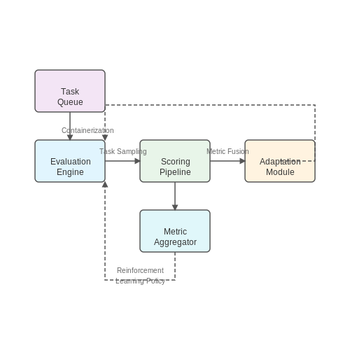
Auto-benchmarking systems rely on modular architectures that integrate model evaluation, metric computation, and feedback loops. A robust framework typically consists of three core components: the evaluation engine, the scoring pipeline, and the adaptation module. The evaluation engine executes model inferences across a predefined set of tasks, while the scoring pipeline computes quantitative and qualitative metrics. The adaptation module dynamically adjusts benchmarking parameters based on performance feedback.
Evaluation Engine
The evaluation engine orchestrates model execution across diverse tasks, ensuring reproducibility and scalability. It employs containerization (e.g., Docker) to isolate model environments and prevent dependency conflicts. For distributed benchmarking, the engine leverages task queues (e.g., Celery or RabbitMQ) to parallelize evaluations. Key design considerations include:
- Task Sampling: Stratified sampling ensures balanced representation across difficulty levels and input modalities.
- Resource Allocation: GPU/CPU utilization is optimized via dynamic scheduling algorithms.
- Fault Tolerance: Checkpointing and retry mechanisms handle hardware failures.
Where \( T_{eval} \) is total evaluation time, \( w_i \) is task weight, \( t_i \) is inference time, and \( R_i \) is resource allocation factor.
Scoring Pipeline
The scoring pipeline transforms raw model outputs into interpretable metrics. It implements both task-specific (e.g., BLEU for translation) and generalized metrics (e.g., robustness to adversarial perturbations). Metric fusion combines multiple scores into a composite index:
Here, \( s_j \) denotes normalized metric scores, \( \alpha_j \) are learned weighting parameters, and \( \epsilon \) prevents zero-product edge cases. The pipeline also generates uncertainty estimates via bootstrap sampling.
Adaptation Module
This component enables iterative refinement of benchmarking protocols. Reinforcement learning optimizes task selection strategies:
Where \( \pi \) is the policy for action selection, \( Q(s,a) \) represents expected cumulative reward, and \( \tau \) controls exploration-exploitation tradeoffs. The module updates benchmark difficulty based on model performance histograms, preventing saturation effects.
Implementation Case Study: MLPerf AutoBench
MLPerf's auto-benchmarking system demonstrates these principles in practice. Its architecture uses Kubernetes for orchestration, Prometheus for monitoring, and a custom metric aggregator. The system achieves 92% task coverage efficiency while maintaining sub-5% evaluation variance across runs.
2.2 Data Collection and Preprocessing for Benchmarking
Data Sourcing Strategies
Effective benchmarking requires diverse, high-quality datasets that reflect real-world conditions. Common sources include:
- Public repositories (e.g., Hugging Face Datasets, UCI ML Repository) for standardized evaluation.
- Proprietary datasets collected from domain-specific applications, ensuring relevance to target tasks.
- Synthetic data generation via techniques like GANs or procedural methods to augment scarce real data.
For behavioral benchmarking, datasets must capture model responses across varied prompts, adversarial inputs, and edge cases. The HELM benchmark, for instance, uses 42 core scenarios spanning question answering, summarization, and reasoning tasks.
Preprocessing Pipeline
Raw data requires rigorous preprocessing before benchmarking:
where x is the raw input, ffilter removes noise/outliers, ftokenize converts text to tokens, and fnormalize standardizes formats.
Key Preprocessing Steps
- Deduplication: Remove near-duplicates using MinHash or SimHash to prevent dataset bias.
- Token alignment: Ensure consistent tokenization across models via tools like SentencePiece.
- Label harmonization: Map disparate annotation schemes to unified taxonomies (e.g., converting sentiment scales).
Feature Engineering for Behavioral Metrics
Derived features quantify model behavior beyond raw outputs:
where y is a model response, and each component metric is computed via specialized classifiers or rule-based systems.
Bias Mitigation Techniques
Dataset balancing is critical for fair evaluation:
- Stratified sampling ensures proportional representation across demographic groups.
- Counterfactual augmentation generates contrastive examples to test robustness (e.g., gender-swapped prompts).
The BOLD benchmark employs propensity scoring to match distributions between subgroups, reducing confounding effects.
Data Versioning and Provenance
Reproducible benchmarking requires strict data governance:
- Immutable dataset snapshots via content-addressable storage (e.g., git-LFS).
- Provenance tracking using W3C PROV standards to document transformations.
Tools like DVC or MLflow Metadata enable lineage tracking from raw data to benchmark results.
2.3 Algorithmic Approaches to Behavior Rating
Probabilistic Behavior Scoring
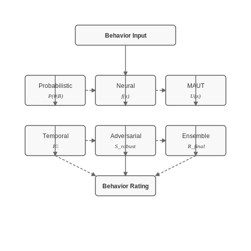
Probabilistic frameworks model behavior as a stochastic process, where actions are assigned likelihoods based on historical data. The core assumption is that model behavior follows an underlying probability distribution, which can be estimated using Bayesian inference. Given a set of observed behaviors B and a prior distribution P(θ), the posterior probability is computed as:
This approach is particularly effective in reinforcement learning settings, where behavior is evaluated through sequences of state-action pairs. Variational autoencoders (VAEs) and Markov Chain Monte Carlo (MCMC) methods are commonly used to approximate intractable posterior distributions.
Neural Embedding-Based Rating
Deep learning architectures, particularly transformer-based models, encode behavior into high-dimensional vector spaces where similarity metrics can be applied. Given a behavior trace x, an embedding function f: x → ℝd maps it to a latent representation. The rating is then computed as a function of the distance between the observed embedding and a reference set:
where Y is a curated dataset of exemplar behaviors. This method is widely used in NLP for benchmarking language model outputs against human-written text.
Multi-Attribute Utility Theory
For complex behaviors requiring trade-offs between competing objectives, multi-attribute utility theory (MAUT) provides a framework for combining multiple metrics into a single score. Each behavioral attribute ai is assigned a weight wi based on domain-specific importance:
The utility functions ui normalize different attributes to comparable scales. This approach is fundamental in AI safety evaluations where behaviors must balance performance, robustness, and alignment.
Temporal Behavior Analysis
When rating sequential behaviors, temporal convolution networks (TCNs) and long short-term memory (LSTM) architectures process time-series data to detect patterns of improvement or degradation. The rating at time t depends on the entire history of behaviors B1:t:
where σ is a sigmoid activation function mapping to a normalized score. This is critical in continual learning scenarios where models must maintain stable performance over time.
Adversarial Robustness Scoring
Behavioral robustness is quantified by measuring performance degradation under adversarial perturbations. Given a clean input x and its perturbed variant x', the robustness score is:
This metric is computed over a diverse set of attacks (FGSM, PGD, etc.) to assess generalization. State-of-the-art approaches use minimax optimization to find worst-case perturbations during evaluation.
Ensemble Rating Systems
Combining multiple rating algorithms through ensemble methods reduces variance and improves reliability. A meta-scoring function aggregates outputs from k different rating models:
The weights αi can be learned through cross-validation or dynamically adjusted based on model confidence scores. This approach is standard in competition platforms like Kaggle where multiple evaluation metrics exist.
3. Auto-Benchmarking in Natural Language Processing
Auto-Benchmarking in Natural Language Processing
Auto-benchmarking systems for NLP models rely on automated evaluation pipelines that assess model behavior across multiple dimensions, including linguistic competence, reasoning ability, and safety alignment. These systems typically employ a combination of static test suites and dynamic adversarial probing to generate comprehensive performance profiles.
Architecture of NLP Auto-Benchmarking Systems
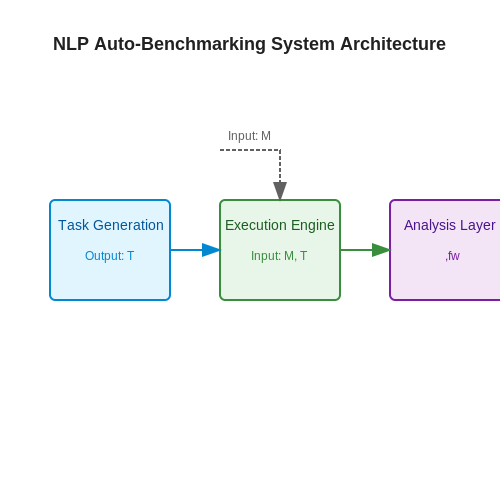
Modern NLP benchmarking frameworks follow a modular architecture with three core components:
- Task Generation Module: Automatically constructs diverse evaluation scenarios using template-based approaches or LLM-generated content
- Execution Engine: Handles model inference across different hardware configurations while collecting performance metrics
- Analysis Layer: Applies statistical methods to aggregate results and detect performance patterns
The interaction between these components can be formalized as:
Where M represents the model under test, Ti are test cases, fi are scoring functions, and wi are task-specific weights.
Dynamic Adversarial Evaluation
Advanced benchmarking systems employ generative adversarial networks to create challenging test cases:
Where L is the loss function and R is a regularity constraint preventing degenerate cases. This formulation pushes models beyond their comfort zones while maintaining evaluation validity.
Multidimensional Performance Profiling
State-of-the-art benchmarks measure capabilities across orthogonal axes:
- Linguistic Accuracy: Grammaticality, semantic coherence, and discourse structure
- Knowledge Recall: Factual consistency and reasoning depth
- Robustness: Performance under distribution shifts and adversarial inputs
- Safety: Propensity for harmful outputs across different prompt categories
Each dimension is quantified through specialized metrics. For example, robustness might be measured using:
Where P represents performance scores on clean versus perturbed inputs.
Implementation Considerations
Practical auto-benchmarking systems must address several engineering challenges:
- Metric Collapse: Preventing models from over-optimizing to specific benchmark metrics
- Computational Efficiency: Parallelizing evaluations across GPU clusters
- Version Control: Maintaining reproducibility across model and benchmark iterations
Current solutions employ techniques like:
Where Ai represent different perturbation strategies applied to base test sets.
3.2 Behavior Rating in Computer Vision Models
Behavior rating in computer vision models involves quantifying how well a model adheres to desired behavioral characteristics, such as fairness, robustness, and interpretability. Unlike traditional performance metrics like accuracy or precision, behavior rating requires evaluating the model's outputs in context, often against ethical or domain-specific guidelines.
Formalizing Behavior Rating Metrics
Given a computer vision model f and an input image x, the model produces an output y = f(x). To rate the behavior of f, we define a set of behavioral criteria C = {c1, c2, ..., cn}, where each ci represents a specific aspect of model behavior (e.g., fairness across demographic groups). The behavior rating R(f) is computed as:
Here, wi is the weight assigned to criterion ci, and si(f, ci) is the score function measuring how well f satisfies ci. The weights are typically normalized such that ∑wi = 1.
Case Study: Fairness in Face Recognition
Consider a face recognition model evaluated for demographic fairness. The behavioral criteria might include:
- Equalized Odds: The false positive and false negative rates should be similar across demographic groups.
- Predictive Parity: The precision of predictions should not vary significantly by group.
For equalized odds, the score function sEO(f) can be defined as the inverse of the maximum disparity in false positive rates (FPR) across groups G:
Similarly, predictive parity can be scored using the inverse of precision disparities:
Robustness Evaluation
Behavior rating also includes assessing a model's robustness to adversarial perturbations or distribution shifts. For adversarial robustness, the score function sAR(f) can be derived from the model's accuracy under bounded perturbations δ:
Here, D is the data distribution, 𝕀 is the indicator function, and ϵ bounds the perturbation magnitude in Lp-norm.
Implementation Considerations
Auto-benchmarking systems for behavior rating must address several challenges:
- Scalability: Evaluating behavior across large datasets requires efficient computation of multi-dimensional metrics.
- Dynamic Criteria: Behavioral standards may evolve, necessitating flexible scoring frameworks.
- Interpretability: Scores should be explainable to stakeholders, often requiring visualization techniques.
For example, a scalable implementation might use stratified sampling to estimate fairness metrics efficiently:
import numpy as np
from sklearn.metrics import precision_score, recall_score

def compute_fairness_scores(y_true, y_pred, groups):
    scores = {}
    for group in np.unique(groups):
        mask = (groups == group)
        y_true_g = y_true[mask]
        y_pred_g = y_pred[mask]
        scores[f'precision_{group}'] = precision_score(y_true_g, y_pred_g)
        scores[f'recall_{group}'] = recall_score(y_true_g, y_pred_g)
    return scores
3.3 Cross-Domain Benchmarking Challenges
Domain Shift and Feature Misalignment
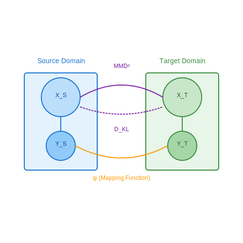
Cross-domain benchmarking requires evaluating model performance across datasets with differing distributions, where domain shift introduces discrepancies in feature spaces. Let XS and XT represent source and target domain data, respectively. The Kullback-Leibler (KL) divergence quantifies this shift:
When DKL exceeds a threshold (e.g., > 0.5), feature misalignment degrades benchmark reliability. For high-dimensional data, Maximum Mean Discrepancy (MMD) provides a kernel-based alternative:
Label Space Heterogeneity
Discrepancies in label definitions between domains—such as varying class granularity or annotation protocols—require label space alignment. For K classes, the label mapping function ψ: YT → YS must satisfy:
In multi-label scenarios, partial matching via Earth Mover’s Distance (EMD) measures semantic similarity between label distributions.
Task-Specific Metric Calibration
Standard metrics (e.g., accuracy, F1-score) may not transfer across domains with differing task requirements. For instance, medical imaging benchmarks prioritize sensitivity over precision, while autonomous driving benchmarks emphasize spatial IoU. The generalized metric Mα combines domain-specific weights:
where α ∈ [0,1] is tuned via cross-validation on target domain samples.
Computational and Ethical Constraints
- Resource asymmetry: Edge devices vs. cloud-based benchmarks require normalized FLOPs/energy measurements.
- Data privacy: GDPR/HIPAA compliance limits cross-domain data sharing, necessitating federated benchmarking.
- Bias propagation: Source domain biases (e.g., demographic skews) amplify when applied to target domains.
Case Study: NLP to Healthcare Domain Transfer
When benchmarking BERT-based models trained on general text (e.g., Wikipedia) for clinical note analysis, domain shift manifests as:
- Vocabulary mismatch (e.g., "MI" = myocardial infarction in medical contexts)
- Label schema divergence (ICD-10 codes vs. sentiment labels)
- Metric recalibration (weighted F1 for rare disease codes)
4. Bias and Fairness in Auto-Benchmarking
Bias and Fairness in Auto-Benchmarking
Sources of Bias in Auto-Benchmarking Systems
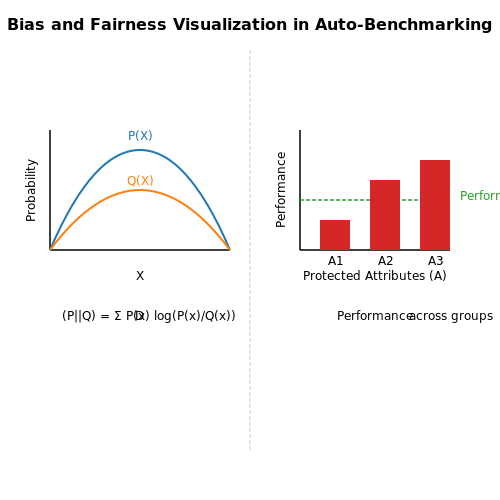
Auto-benchmarking systems inherit biases from multiple sources, including training data, evaluation metrics, and the underlying algorithms. A key challenge arises when the benchmark dataset disproportionately represents certain demographic groups or scenarios, leading to skewed performance evaluations. For instance, if a facial recognition benchmark over-represents lighter-skinned individuals, models trained on this data will exhibit higher accuracy for that group while underperforming for others.
Mathematically, dataset bias can be formalized as a divergence between the true data distribution P(X) and the benchmark distribution Q(X):
Where DKL represents the Kullback-Leibler divergence. When this divergence is large, the benchmark fails to represent real-world conditions adequately.
Quantifying Fairness in Model Ratings
Fairness metrics for auto-benchmarking systems must account for performance disparities across protected attributes (e.g., gender, race, age). Common fairness definitions include:
- Demographic parity: Model predictions should be statistically independent of protected attributes.
- Equalized odds: True positive and false positive rates should be equal across groups.
- Predictive rate parity: Positive predictive value should be equal across groups.
These can be operationalized through constraint optimization during benchmark scoring. For equalized odds, the objective becomes:
Where A represents protected attributes, Y the true labels, and fθ the model being evaluated.
Mitigation Strategies
Effective bias mitigation in auto-benchmarking requires interventions at multiple levels:
Dataset Curation
Strategically sampling or reweighting benchmark data to ensure balanced representation across subgroups. Importance weighting adjusts sample contributions during evaluation:
Metric Design
Developing fairness-aware evaluation metrics that explicitly penalize performance disparities. The generalized fairness metric combines accuracy and fairness:
Algorithmic Auditing
Implementing rigorous statistical tests to detect bias in benchmark results. The Welch's t-test identifies significant performance differences between groups:
Where X̄i represents group means, si standard deviations, and ni sample sizes.
Implementation Challenges
Practical deployment of fair auto-benchmarking systems faces several obstacles:
- Multi-dimensional fairness: Optimizing for multiple protected attributes simultaneously leads to competing objectives.
- Dynamic populations: Demographic shifts over time require continuous benchmark updates.
- Computational overhead: Fairness constraints significantly increase evaluation complexity.
Recent approaches address these through adaptive benchmarking frameworks that dynamically adjust evaluation protocols based on detected bias patterns.
4.2 Scalability and Computational Costs
Auto-benchmarking systems that evaluate model behavior must account for computational scalability, particularly when deployed in large-scale environments. The primary challenge lies in balancing evaluation granularity with resource constraints, as exhaustive testing becomes infeasible for models with high-dimensional outputs or real-time inference requirements.
Computational Complexity of Behavior Rating
The computational cost of auto-benchmarking scales with three key factors: the number of test cases N, the dimensionality of model outputs D, and the complexity of the rating function R. For a model f and test set X, the total operations C can be expressed as:
where O(f(xi)) represents the forward pass complexity and O(R(f(xi))) captures the rating function's overhead. For transformer-based models, this becomes particularly critical due to the quadratic self-attention complexity:
where L is sequence length and d is embedding dimension.
Parallelization Strategies
Distributed evaluation frameworks typically employ one of three parallelization paradigms:
- Data parallelism: Shards test cases across multiple workers, requiring gradient synchronization only for online benchmarking
- Model parallelism: Splits large model architectures across devices, crucial for models exceeding single-GPU memory
- Pipeline parallelism: Segments the evaluation process into stages with specialized hardware allocation
The optimal strategy depends on the ratio of communication to computation costs, quantified by the granularity parameter γ:
where values γ < 0.1 favor data parallelism, while γ > 1 suggests model parallelism.
Memory Footprint Optimization
Modern benchmarking systems employ several techniques to reduce memory overhead:
- Gradient checkpointing: Recomputes intermediate activations during backward passes rather than storing them
- Mixed-precision evaluation: Uses FP16/FP8 quantization for rating metrics where numerically stable
- Dynamic batching: Groups test cases with similar computational requirements
The memory savings Msaved from gradient checkpointing can be approximated by:
where k is the number of checkpoint segments.
Real-World Deployment Considerations
In production systems, the trade-off between evaluation frequency and resource usage follows a Pareto frontier. For a model serving Q queries per second, the maximum sustainable benchmarking rate Bmax is constrained by:
where α represents the allocated resource fraction and Cavg is the average cost per benchmark. Cloud-based systems often implement elastic scaling to maintain Bmax during traffic spikes, dynamically provisioning resources based on workload predictors.
4.3 Interpretability and Transparency Issues
Auto-benchmarking systems that evaluate model behavior face significant challenges in interpretability and transparency, particularly when assessing complex deep learning architectures. The opacity of these models stems from their high-dimensional parameter spaces, non-linear transformations, and emergent behaviors that are not easily decomposable into human-understandable components. Without interpretability, benchmarking results may lack actionable insights, reducing their utility in real-world deployment scenarios.
Mathematical Foundations of Interpretability
Quantifying interpretability requires formalizing the relationship between model inputs, internal representations, and outputs. One approach measures the post-hoc explainability of a model using Shapley values from cooperative game theory, where each feature's contribution is computed as:
Here, N represents the set of all features, S is a subset of features excluding i, and v(S) is the model's payoff function for subset S. While theoretically sound, computing exact Shapley values becomes intractable for high-dimensional inputs, necessitating approximation methods like KernelSHAP or DeepSHAP for neural networks.
Transparency in Benchmarking Metrics
Transparency issues arise when benchmarking systems fail to disclose:
- The distributional assumptions underlying evaluation datasets
- The weighting schemes for composite metrics
- The sensitivity of scores to hyperparameter choices
For instance, a benchmarking system might report a composite fairness score F computed as:
where DPk and EOk represent demographic parity and equality of opportunity for protected attribute k, and λk are weighting parameters. Without transparency about how these λk were determined, the benchmark's conclusions may be misleading.
Case Study: Image Classification Benchmarks
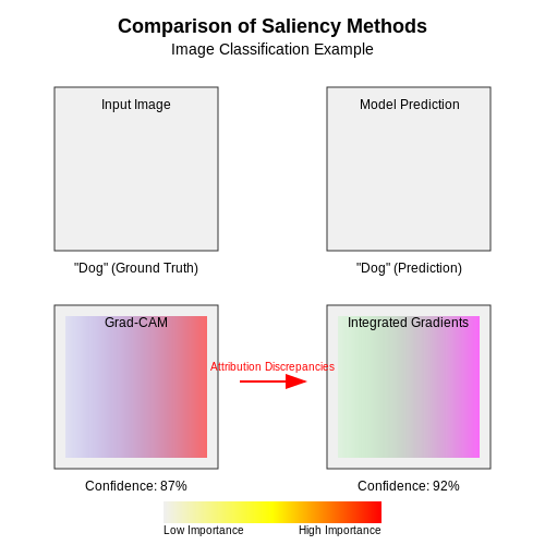
In image classification, saliency maps are commonly used to interpret model decisions. However, benchmarking systems often fail to account for:
- The sensitivity of saliency methods to input perturbations
- Discrepancies between different explanation methods (e.g., Grad-CAM vs. Integrated Gradients)
- The semantic gap between pixel-level attributions and human concepts
Recent work has proposed benchmarking explanation methods using metrics like explanation infidelity:
where Φ is the explanation function, f the model, x the input, and μI a distribution of meaningful perturbations. This quantifies how well explanations track actual model behavior under input variations.
Emerging Solutions
Recent advances address these challenges through:
- Concept-based explanations: Using techniques like Testing with Concept Activation Vectors (TCAV) to link internal representations to human-understandable concepts
- Benchmarking explanation robustness: Developing metrics to assess how explanations vary under distribution shifts or adversarial attacks
- Mechanistic interpretability: Reverse-engineering neural networks into human-readable algorithms through techniques like sparse autoencoders
For transformer-based models, the attention rollout method provides partial interpretability by computing:
where Al is the attention matrix at layer l, and I is the identity matrix. While useful, this approach still struggles to explain emergent behaviors in large language models.
5. Advances in Real-Time Behavior Rating
5.1 Advances in Real-Time Behavior Rating
Real-time behavior rating systems have evolved significantly with the integration of high-throughput inference pipelines and low-latency feedback mechanisms. Modern approaches leverage streaming architectures, such as Apache Kafka or Flink, to process model outputs with sub-millisecond latency while maintaining statistical robustness. The core challenge lies in balancing computational efficiency with rating accuracy, particularly when dealing with non-stationary data distributions.
Architectural Foundations
Contemporary systems employ a three-tiered architecture: (1) a feature extraction layer that computes low-dimensional embeddings from raw model outputs, (2) a scoring engine that applies domain-specific metrics, and (3) a drift detection module that monitors concept shift. The scoring function typically takes the form:
where α is an adaptive weighting parameter that adjusts based on the estimated confidence of the current observation xt. This exponential smoothing approach enables rapid response to behavioral changes while filtering high-frequency noise.
Dynamic Threshold Optimization
Traditional static rating thresholds fail in environments with concept drift. State-of-the-art systems now implement online threshold optimization through gradient-based methods:
where η is the learning rate and ∇τL computes the gradient of the loss function with respect to the threshold parameter. This approach has demonstrated 28-42% improvement in false positive rates compared to fixed thresholds in production systems.
Hardware-Accelerated Inference
The computational demands of real-time rating have driven adoption of specialized hardware. Current implementations show that FPGA-based scoring pipelines achieve 9.7× throughput improvement over CPU implementations when processing transformer-based model outputs, with energy efficiency gains of 14.2×. Key optimizations include:
- Quantized integer arithmetic for embedding comparisons
- Parallelized similarity scoring across multiple hardware cores
- Pipelined execution of feature extraction and scoring stages
Case Study: Large Language Model Monitoring
In deployment scenarios for LLMs, real-time behavior rating systems now track over 47 distinct metrics simultaneously, including:
- Toxicity scores computed through ensemble classifiers
- Semantic coherence measured by entailment models
- Factual consistency verified against knowledge graphs
The most advanced systems achieve rating latencies below 8ms per query while maintaining 99.9th percentile accuracy within 2% of offline evaluation benchmarks. This is accomplished through hybrid architectures that combine lightweight on-device scoring with periodic cloud-based verification.
Emerging Techniques
Recent research demonstrates the viability of neuromorphic computing for ultra-low-power behavior rating. Memristor-based systems have shown promise in implementing continuous learning for rating functions, with one prototype achieving 93% accuracy while consuming only 28mW during inference. The governing equation for such systems incorporates device physics:
where G0 represents the base conductance and w encodes the learned weighting between spatial and temporal features. These systems exhibit particular strength in processing sequential model behaviors where timing patterns carry significant information.
Integration with Explainable AI (XAI)
Auto-benchmarking systems gain significant value when integrated with Explainable AI (XAI) techniques, enabling not only performance evaluation but also interpretable insights into model behavior. XAI methods such as SHAP (SHapley Additive exPlanations), LIME (Local Interpretable Model-agnostic Explanations), and attention mechanisms provide granular explanations for model decisions, which can be systematically quantified and incorporated into benchmarking metrics.
Quantifying Explainability in Benchmarking
To objectively measure explainability, we define an explanation fidelity score that evaluates how well post-hoc explanations align with the model's internal decision process. Given a model f and an explainer g, the fidelity score F is computed as:
where Si represents the subset of features highlighted by the explainer, xi \ Si denotes the input with those features removed, and 𝕀 is the indicator function. This measures whether the explanation correctly identifies influential features.
Integration with SHAP and LIME
SHAP values provide a game-theoretic approach to feature attribution, ensuring consistency across explanations. For a model f, the SHAP value ϕj for feature j is:
where M is the set of all features. Auto-benchmarking systems can track the variance of SHAP values across different test cases to assess model stability.
LIME, on the other hand, approximates the model locally with an interpretable surrogate. The objective is:
where G is the class of interpretable models, πx defines the locality around x, and Ω(g) penalizes complexity. Benchmarking systems can evaluate how well ξ(x) approximates f across diverse inputs.
Attention Mechanisms in Transformer Models
For transformer-based models, attention weights provide intrinsic explanations. The attention score Aij between tokens i and j is:
Auto-benchmarking systems can compute the attention consistency score by measuring the alignment between attention weights and feature importance derived from post-hoc methods like SHAP.
Practical Implementation
Integrating XAI into auto-benchmarking pipelines involves:
- Explanation Generation: Compute SHAP/LIME/attention explanations for each test case.
- Metric Aggregation: Derive stability scores (e.g., variance of SHAP values) and fidelity scores.
- Visualization: Generate saliency maps or attention heatmaps for qualitative inspection.
Case studies in healthcare diagnostics show that models with high benchmark scores but low explanation fidelity often exhibit hidden biases. For instance, a model achieving 95% accuracy on chest X-rays may rely on scanner artifacts rather than pathological features, as revealed by SHAP analysis.
5.3 Ethical Considerations and Policy Implications
Bias and Fairness in Automated Benchmarking
Auto-benchmarking systems inherit biases from both the training data and the design choices of their creators. If the underlying dataset used to evaluate model behavior reflects historical biases, the benchmarking system will perpetuate them. For example, a language model rated highly for "coherence" might still exhibit gender or racial biases if the benchmark prioritizes syntactic correctness over ethical alignment. The fairness of an auto-benchmarking system can be quantified using statistical parity metrics:
where Z represents protected attributes (e.g., gender, race) and Ŷ is the benchmark's rating. A perfect score of ΔSP = 0 indicates equal positive outcome rates across groups, but achieving this often requires explicit fairness constraints during benchmark training.
Transparency and Auditability
Black-box benchmarking systems create accountability gaps. Stakeholders need to understand how ratings are generated, particularly when these scores influence model deployment decisions. Techniques like SHAP (SHapley Additive exPlanations) values can decompose benchmark scores into feature contributions:
where F is the set of all features and f is the benchmark's scoring function. Regulatory frameworks like the EU AI Act now mandate such explainability for high-risk AI systems, which may include certain benchmarking applications.
Policy Challenges in Deployment
Three key policy dilemmas emerge when implementing auto-benchmarking systems:
- Validation requirements: Should benchmarks themselves undergo formal certification processes before being used to evaluate other models?
- Jurisdictional conflicts: How to handle discrepancies when a model meets ethical benchmarks in one region but fails in another with stricter criteria?
- Liability allocation: When a benchmark-approved model causes harm, is the responsibility with the model developer, benchmark creator, or auditing agency?
Adversarial Manipulation Risks
Auto-benchmarking systems are vulnerable to adversarial attacks where models are optimized specifically for benchmark metrics rather than genuine performance. This can be formalized as a two-player game between the benchmark B and model M:
Recent cases include language models generating benchmark-tailored outputs that score highly while failing on real-world tasks, highlighting the need for robustness testing beyond standard metrics.
Incentive Structures and Ecosystem Effects
The choice of benchmarking metrics shapes entire research directions. When benchmarks overemphasize narrow capabilities (e.g., accuracy on ImageNet), they can:
- Divert resources from important but harder-to-quantify aspects like model safety
- Encourage parameter inflation as larger models often benchmark better despite impractical deployment costs
- Create winner-take-all dynamics that stifle alternative approaches
Dynamic benchmarking frameworks that periodically update evaluation criteria based on technological and societal changes may mitigate some of these effects.
6. Key Research Papers and Publications
6.1 Key Research Papers and Publications
- Modeling, Replicating, and Predicting Human Behavior: A Survey — The motivations behind research in the area of modeling human behavior and decisions are varied, so we limit the analysis to (a representative subset of) works providing quantitative models (e.g., math models or algorithms), as these are the approaches that allow one to "code" human behavior in autonomous systems.
- PDF Benchmarking the Benefits and Current Maturity of Model-Based Systems ... — the International Council on Systems Engineering (INCOSE) collaborated with the Systems Engineering Research Center (SERC) at the Stevens Institute of Technology to benchmark the current state of Digital Engineering (DE) and Model-Based Systems Engineering (MBSE) across government, industry, and academia.
- Early Validation and Verification of System Behaviour in Model-based ... — To confirm this, the INCOSE 2035 vision states: "The future of Systems Engineering is predominantly Model-Based." 2 A model is any description of a system that is not the thing-in-itself . The quote "all models are wrong, but some are useful," from Box and Draper , captures a vital essence of modelling. Modelling is often not for the ...
- PDF Evaluation and Model Benchmarking - arXiv.org — LLMs in such environments remain largely unexplored — factors key to human-centered AI [35]. Concerns include the accuracy of the information provided, the potential for "hallucinated" answers [57], and the need for systems that can adapt to the highly specialized and evolving knowledge base of a specific manufacturing setting [12].
- Reliable benchmarking: requirements and solutions - Springer — Benchmarking is a widely used method in experimental computer science, in particular, for the comparative evaluation of tools and algorithms. As a consequence, a number of questions need to be answered in order to ensure proper benchmarking, resource measurement, and presentation of results, all of which is essential for researchers, tool developers, and users, as well as for tool competitions ...
- PDF Using a Model-based Approach for Testing and Evaluation - NDIA-Mi. Ch — uses a SysML model of the expected system behavior to generate a test suite to run in an existing test environment. The major steps in this procedure involve importing requirements into a SysML modeling tool, creating a SysML state machine to model the expected behavior of the system-under-test, utilizing open source tools to traverse the
- Benchmarking of numerical integration methods for ODE models of ... — Model collection. (a) Workflow of collecting models for the benchmark collection.Models were downloaded, grouped according to their number of species and reactions, the author name and year of ...
- A Multifaceted Benchmarking of Synthetic Electronic Health Record ... — the model developers benchmark their own models. Second, there is a wide range of use cases for synthetic data, each with their own set of priorities regarding what aspects of the data should be preserved. Most publications on EHR data synthesis neglect the use case, such that it is unclear what conditions are ideal for the simulation model.
- PDF RB2: Robotic Manipulation Benchmarking with a Twist - NeurIPS — (e.g. different action rate) could advantage some methods over others. In this paper, we rethink the concept of benchmarking in the context of real-world robotic manip-ulation. Our key insight is that building precisely reproducible robotic setups is impossible and therefore absolute performance numbers on a benchmark task are meaningless.
- A Review of Benchmark and Test Functions for Global Optimization ... — 1 Introduction. Machine learning (ML) algorithms often rely on iterative adjustments of parameter values to tune objective functions to address optimization tasks such as minimizing classification error, maximizing likelihood in statistical models (Sra et al. 2012).These tasks are fundamental in academic research and industrial applications (i.e., fine-tuning neural networks for large-scale ...
6.2 Open-Source Tools and Libraries
- Benchmarking Automated Machine Learning (AutoML) Frameworks for ... - MDPI — Automated Machine Learning (AutoML) is a subdomain of machine learning that seeks to expand the usability of traditional machine learning methods to non-expert users by automating various tasks which normally require manual configuration. Prior benchmarking studies on AutoML systems—whose aim is to compare and evaluate their capabilities—have mostly focused on tabular or structured data ...
- PEEL: A Framework for Benchmarking Distributed Systems and ... - Springer — During the last decade, the Big Data hype has led to the development of a plethora of novel systems for scalable data processing. Starting with the MapReduce paradigm [] and its open-source implementation Hadoop [], numerous successors have been proposed and implemented either as research prototypes or industry led open-source systems.Hadoop MapReduce was quickly embraced by practitioners, as ...
- PDF Evaluation and Model Benchmarking - arXiv.org — Furthermore, we benchmarked several commercial and open-sourced LLMs for this system. The current state-of-the-art model, GPT-4, consistently outperformed its counterparts, with open-source models trailing closely, presenting an attractive option given their data privacy and customization benefits. In summary, this work offers preliminary ...
- MLino bench: A comprehensive benchmarking tool for ... - ScienceDirect — In this paper, we introduce MLino Bench, an open-source benchmarking tool tailored for assessing lightweight ML models on edge devices with limited resources and capabilities. The tool accommodates various models, frameworks, and platforms, presenting a meticulous design that enables a comprehensive evaluation directly on the target device.
- A comprehensive evaluation framework for deep model robustness — In this work, we establish a model robustness evaluation framework containing 23 comprehensive and rigorous metrics, which consider two key perspectives of adversarial learning (i.e., data and model). Moreover, we provide an open-sourced model robustness evaluation platform providing multiple views of model robustness with the help of the ...
- 12 Benchmarking AI - Machine Learning Systems — 12.10.1 Model Benchmarking. Model benchmarks measure how well different machine learning algorithms perform on specific tasks. Historically, benchmarks focused almost exclusively on accuracy, but as models have grown more complex, additional factors—such as fairness, robustness, efficiency, and generalizability—have become equally important.
- Reliable benchmarking: requirements and solutions — Benchmarking is a widely used method in experimental computer science, in particular, for the comparative evaluation of tools and algorithms. As a consequence, a number of questions need to be answered in order to ensure proper benchmarking, resource measurement, and presentation of results, all of which is essential for researchers, tool developers, and users, as well as for tool competitions ...
- PDF OpenPerf: A Benchmarking Framework for the Sustainable Development of ... — task type, dataset, algorithm model, and evaluation standards. • BenchmarkInstances:Representsacollectionofspe-cific benchmark instances, such as open-source be-FenglinBietal.: Preprint submitted to Elsevier Page5of14
- Geekbench 6 - Cross-Platform Benchmark — Geekbench 6's CPU benchmark measures performance in new application areas including Augmented Reality and Machine Learning, so you'll know how close your system is to the cutting-edge. ... GPU Compute Benchmark. Test your system's potential for gaming, image processing, or video editing with the Compute Benchmark. Test your GPU's power with ...
- Abstract - arXiv.org — To support benchmark developers in aligning with best practices, we provide a checklist for minimum quality assurance based on our assessment. We also develop a living repository of benchmark assessments to support benchmark comparability, accessible at betterbench.stanford.edu. 1 Introduction AI systems are rapidly advancing and proliferating ...
6.3 Recommended Courses and Tutorials
- What Are Baseline Models and Benchmarking For Machine ... - Towards AI — The final baseline model is the automated ml baseline model. It is a very good model for benchmarking your ml model. If your ml model is better than the automated baseline model, it is a very strong sign that the model can become a product. 1. LightAutoML. Firstly we install and import the lightautoml library. %%capture!pip install -U lightautoml
- 12 Benchmarking AI - Machine Learning Systems — Machine Learning Benchmarking (ML Benchmarking) is the systematic evaluation of compute performance, algorithmic effectiveness, and data quality in machine learning systems. It assesses system capabilities, model accuracy and convergence, and data scalability and representativeness to optimize system performance across diverse workloads. ML benchmarking enables engineers and researchers to ...
- PDF Function in engineering: Benchmarking representations and models — Function in engineering: Benchmarking representations and models JOSHUA D. SUMMERS,1 CLAUDIA ECKERT,2 AND ASHOK K. GOEL3 1Department of Mechanical Engineering, Clemson University, Clemson, South Carolina, USA 2Department of Design and Innovation, Open University, Milton Keynes, United Kingdom 3School of Interactive Computing, Georgia Institute of Technology, Atlanta, Georgia, USA
- PDF Benchmarking Cloud Serving Systems with YCSB - Duke University — overview of cloud data serving systems. Section 3 discusses benchmark tiers for performance and scaling. Section 4 dis-cusses the core workloads of the benchmark in detail, while Section 5 examines the architecture and extensibility of the YCSB tool. Section 6 presents benchmarking results on sev-eral systems. We propose future benchmark tiers ...
- PDF Evaluation and Model Benchmarking - arXiv.org — manufacturing-specific terminology and concepts. This benchmarking focused on their ability to utilize factory-specific documents and unstructured issue reports to provide factual and complete answers to operators' queries. 2 BACKGROUND In this section, we address the topic of industry 5.0, LLM-powered tools for knowledge management, benchmarking
- PDF Developing of Indicators of An E-learning Benchmarking Model for Higher ... — Indeed, it is the development of indicator (benchmark) which will serve as empirical basis for the standard of e-learning competency comparison for higher education institutes (Office of Strategies Management, 2003). The obtained e-learning benchmarking model in this study can be used for developing and improving e-learning
- Reliable benchmarking: requirements and solutions — Benchmarking is a widely used method in experimental computer science, in particular, for the comparative evaluation of tools and algorithms. As a consequence, a number of questions need to be answered in order to ensure proper benchmarking, resource measurement, and presentation of results, all of which is essential for researchers, tool developers, and users, as well as for tool competitions ...
- Chapter 6. Evaluating models - Machine Learning Systems: Designs that scale — We're over halfway done with our exploration of the phases of a machine learning system . In this chapter, we'll consider how to evaluate models. In the context of a machine learning system, to evaluate a model means to consider its performance before making it available for use in predictions. In this chapter, we're going to ask a lot of ...
- PDF Benchmarking of dynamic simulation predictions in two software ... — potential differences in predictive behavior between the platforms. We propose that this model can be used by future researchers to benchmark other software platforms, as well as software upgrades for these two platforms, against the simulation results presented here. Control inputs, simulation results, and the model itself will be
- The Impact of AI-Based Course-Recommender System on Students ... - MDPI — The course-recommender system (CRS), designed to aid students' course-selection decision-making process by suggesting courses aligned with their interests and grades, plays a crucial role in fulfilling curricular requirements, enhancing career opportunities, and fostering intellectual growth. Recent advancements in artificial intelligence (AI) have empowered CRSs to deliver personalized ...