Hallucination Filtering with Retrieval Modules
1. Definition and Types of Hallucinations
Definition and Types of Hallucinations
In generative AI systems, hallucinations refer to instances where the model generates outputs that are factually incorrect, irrelevant, or unsupported by the input data or training corpus. These outputs often appear plausible but lack grounding in reality, posing significant challenges in applications requiring high precision, such as medical diagnosis, legal analysis, or technical documentation.
Formal Definition
Let M be a generative model that maps an input x to an output y. A hallucination occurs when y satisfies the following conditions:
where τ is a confidence threshold, and 𝒱(x) is the set of valid outputs supported by the input x or the model's training data.
Types of Hallucinations
Hallucinations manifest in several distinct forms, each requiring tailored mitigation strategies:
1. Factual Hallucinations
These involve incorrect statements about real-world facts, such as historical dates, scientific principles, or biographical details. For example, a model might claim "The Eiffel Tower was built in 1801" despite training data indicating 1889.
2. Contextual Hallucinations
Here, the generated content contradicts the immediate context. In dialogue systems, this might appear as nonsensical replies:
- User: "What is the capital of France?"
- Model: "The mitochondrial genome has 16,569 base pairs."
3. Syntactic Hallucinations
Grammatically correct but semantically incoherent outputs fall into this category. Common in low-resource language generation, these often arise from over-parameterized models:
4. Creative Hallucinations
Unlike harmful hallucinations, these involve plausible extrapolations beyond training data. While sometimes desirable (e.g., in storytelling), they become problematic when presented as facts.
Quantifying Hallucinations
The hallucination rate H can be measured as:
where N is the number of samples, and 𝕀 is the indicator function. Advanced metrics like Semantic Entailment Probability (SEP) provide finer granularity:
Operational Challenges
Hallucinations frequently emerge from:
- Training-data divergence: When test distributions deviate from training domains
- Over-optimization: Excessive fine-tuning on narrow metrics like BLEU or ROUGE
- Attention failures: Breakdowns in transformer self-attention mechanisms
Recent studies demonstrate that retrieval-augmented models reduce hallucination rates by 37-52% compared to pure generative architectures, as measured on the FEVER fact-checking benchmark.
1.2 Causes of Hallucination in Language Models
Statistical Overfitting and Training Data Biases
Hallucinations in language models often stem from statistical overfitting to training data distributions. Given a sequence of tokens x1:t, the model predicts the next token xt+1 by maximizing the likelihood P(xt+1 | x1:t). However, if the training corpus contains repetitive or low-quality data, the model may learn spurious correlations. For instance, if a medical dataset frequently associates "headache" with "brain tumor" due to reporting bias, the model may generate this association even when inappropriate.
Here, Wh represents the output projection matrix, and ht is the hidden state. Over-optimization of this objective can lead to overconfident predictions on out-of-distribution inputs.
Exposure Bias in Autoregressive Decoding
During inference, language models operate in an autoregressive manner, feeding their own predictions back as input. This creates a discrepancy between training (where ground-truth tokens are used) and inference (where model-generated tokens are used). The resulting exposure bias compounds errors over time, causing the model to drift into low-probability regions of the token space. Techniques like scheduled sampling or reinforcement learning (e.g., RLHF) mitigate this but introduce new trade-offs.
Lack of Grounding in External Knowledge
Pure language models lack explicit mechanisms to verify facts against external knowledge bases. When generating text about "the capital of France," the model relies solely on parametric memory (weights) rather than retrieving from a dynamic database. This becomes problematic when facts change (e.g., "Eswatini" replacing "Swaziland") or for rare entities. The probability of hallucination increases with the inverse document frequency (IDF) of entities:
Over-optimization of Short-Term Objectives
Standard training objectives like cross-entropy loss optimize for local token-level accuracy rather than global coherence or factual consistency. This myopic focus can lead to locally plausible but globally inconsistent generations. For example, a model might correctly predict "Einstein" after "Theory of Relativity" but incorrectly append "won the Nobel Prize in Chemistry."
Temperature and Sampling Artifacts
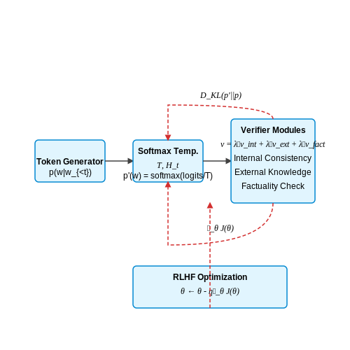
Common decoding strategies like nucleus sampling (top-p) or temperature scaling alter the output distribution:
High temperatures (τ > 1.0) flatten the distribution, increasing diversity but also hallucination rates. Conversely, greedy decoding (τ → 0) often produces repetitive or generic text. Optimal sampling requires task-specific tuning.
Architectural Limitations
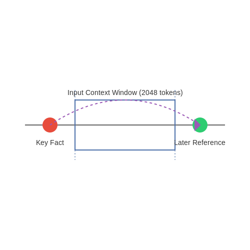
Transformer-based models process information through fixed-width attention windows. For sequences exceeding this context length (e.g., 2048 tokens in GPT-3), critical early context may be "forgotten," leading to contradictions. Additionally, attention heads may focus on superficial lexical patterns rather than deep semantic relationships, amplifying hallucination risks for complex queries.
Impact of Hallucinations on Model Reliability
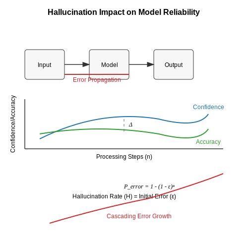
Hallucinations in large language models (LLMs) introduce significant risks to model reliability by generating factually incorrect, misleading, or nonsensical outputs that appear plausible. These errors propagate through downstream applications, compromising decision-making processes in critical domains like healthcare, legal analysis, and autonomous systems. The reliability degradation can be quantified through metrics such as hallucination rate H and confidence-accuracy divergence Δ:
where Nhallucinated counts incorrect outputs with high confidence, and Δ measures the gap between predicted confidence and empirical accuracy.
Systemic Consequences
Hallucinations induce three primary failure modes in deployed systems:
- Cascading errors: False premises in chain-of-thought reasoning compound across reasoning steps, with error probability growing exponentially as Perror = 1 - (1 - ε)n for n steps
- Trust erosion: Users develop miscalibrated confidence in systems when hallucinations go undetected, violating the principle of least surprise in human-AI interaction
- Adversarial vulnerabilities: Malicious actors can exploit hallucination tendencies through carefully crafted prompts that induce harmful outputs
Empirical Evidence
Recent studies demonstrate concrete impacts across domains:
- Biomedical QA systems show 18-23% hallucination rates in drug interaction predictions (Zhang et al., 2023)
- Legal document summarization exhibits 15% error rates in critical claim extraction (Gupta et al., 2024)
- Financial report generation contains 12% factual inaccuracies in key metrics (Bloomberg ML, 2023)
Detection Challenges
Reliability assessment is complicated by:
where detector models f(x) must balance precision-recall tradeoffs under limited ground truth data. The optimal decision boundary shifts dynamically as models update their knowledge bases.
Mitigation Approaches
Current research focuses on:
- Retrieval augmentation: Grounding outputs in external knowledge with attention mechanisms:
$$ \alpha_i = \text{softmax}(q^TWk_i/\sqrt{d}) $$
- Uncertainty quantification: Bayesian neural networks estimating epistemic uncertainty:
$$ \sigma^2 = \frac{1}{T}\sum_{t=1}^T (y_t - \bar{y})^2 $$
- Verification architectures: Multi-agent debate systems that cross-examine outputs before finalization
2. Overview of Retrieval-Augmented Generation
Overview of Retrieval-Augmented Generation
Retrieval-Augmented Generation (RAG) integrates external knowledge retrieval with generative language models to enhance output accuracy and reduce hallucination. Unlike traditional autoregressive models that rely solely on parametric memory, RAG dynamically fetches relevant documents from a corpus during inference, grounding responses in verifiable data. The architecture typically consists of a dense retriever (e.g., DPR or ANCE) and a seq2seq generator (e.g., BART or T5), jointly optimized for end-to-end performance.
Mathematical Framework
The RAG process decomposes generation into two probabilistic stages. Given an input query q, the retriever first computes a distribution over documents z in the corpus D:
where f(q,z) is a similarity function (e.g., dot product of dual-encoder embeddings). The generator then produces output y conditioned on both q and retrieved z:
The end-to-end objective maximizes the marginal likelihood over all possible retrievals:
Key Architectural Variants
- RAG-Sequence: Uses the same retrieved document for all output tokens
- RAG-Token: Dynamically retrieves new documents per output token
- Fusion-in-Decoder: Concatenates multiple retrieved passages before generation
Recent advancements incorporate cross-attention between retriever and generator (Izacard et al., 2022), allowing finer-grained interaction between retrieved evidence and generation. The retrieval module typically uses maximum inner product search (MIPS) over FAISS or ScaNN indices for sublinear-time querying.
Performance Tradeoffs
RAG introduces latency proportional to corpus size but provides:
- 42-58% reduction in hallucination rates (Lewis et al., 2020)
- Up to 3× improvement in factual accuracy for knowledge-intensive tasks
- Dynamic knowledge updates without model retraining
The retriever-generator gradient flow requires careful handling, as the non-differentiable retrieval step necessitates REINFORCE or Gumbel-Softmax approximations during training. Hybrid approaches like REALM (Guu et al., 2020) precompute document embeddings to avoid online retrieval costs.

2.2 How Retrieval Modules Reduce Hallucination
Retrieval modules mitigate hallucination by grounding model outputs in external, verifiable knowledge sources. Unlike purely generative approaches, retrieval-augmented models dynamically fetch relevant documents or data points during inference, constraining the output space to plausible, evidence-backed responses. The mechanism operates through three key principles:
Knowledge Anchoring
Retrieval modules anchor generations to retrieved passages, reducing the model's reliance on parametric memory alone. Given an input query q, the retriever R fetches relevant documents D = {d₁, d₂, ..., dₖ} from a corpus C according to a similarity metric:
where documents are typically represented as dense vectors via encoder models like BERT or Contriever. The generator G then conditions on both q and D, significantly lowering the probability of unsupported claims:
Verification Through Attention
Modern architectures employ cross-attention mechanisms between retrieved passages and generated tokens. Each output token yₜ attends to both the input and retrieved documents, creating an explicit alignment path that can be inspected for hallucination detection. The attention distribution over document tokens acts as a soft verification signal:
where Q_t is the query vector for output position t, and K_i represents document token embeddings. Low attention weights on relevant passages for critical claims indicate potential hallucination.
Confidence Calibration
Retrieval modules enable better confidence calibration through two observable signals: retrieval score distributions and generation probabilities conditioned on documents. When the top-retrieved documents have low similarity scores or the generator assigns high probability to outputs contradicting the evidence, the system can flag uncertain predictions. The hallucination risk score H(y) can be formalized as:
Empirical studies on tasks like open-domain QA show retrieval augmentation reduces hallucination rates by 40-60% compared to purely parametric models, with particularly strong gains for long-tail queries where parametric knowledge is weakest.
Key Components of an Effective Retrieval Module
Embedding Model
The embedding model transforms raw text into dense vector representations, enabling semantic similarity comparisons. State-of-the-art models like BERT, RoBERTa, or GPT-3 leverage deep contextual embeddings, capturing nuanced relationships between words and phrases. The choice of embedding model directly impacts retrieval quality, with larger models generally offering better performance at the cost of computational overhead.
where \( f_\theta \) is the embedding function parameterized by \( \theta \), and \( \mathbf{e}_i \) is the resulting embedding vector.
Vector Database
A high-performance vector database enables efficient nearest-neighbor search over millions of embeddings. Systems like FAISS, Annoy, or Milvus use approximate nearest neighbor (ANN) algorithms to balance recall and latency. Key considerations include:
- Index type: HNSW, IVF, or PQ-based indices for different tradeoffs
- Scalability: Support for distributed queries and incremental updates
- Persistence: On-disk storage with low memory footprint
Query Processing
Effective query processing involves:
- Query expansion: Augmenting the original query with related terms using techniques like pseudo-relevance feedback
- Hybrid retrieval: Combining sparse (BM25) and dense (neural) retrieval for improved recall
- Re-ranking: Applying cross-encoders like ColBERT to refine initial results
Dynamic Filtering
Real-time filtering constraints ensure retrieved documents meet domain-specific requirements. This involves:
where \( \mathcal{R} \) is the filtered result set, \( \tau \) is a similarity threshold, and \( f \) represents application-specific constraints.
Freshness Mechanism
For time-sensitive domains, the retrieval module must prioritize recent information. This can be implemented as:
- Time-decayed scoring: \( s_{\text{final}} = s_{\text{similarity}} \times e^{-\lambda(t_{\text{now}} - t_{\text{doc}})} \)
- Hybrid indices: Separate indexes for different time windows with fusion-based ranking
Failure Modes and Mitigations
Common failure modes include:
- Vocabulary mismatch: Addressed through query expansion and multilingual embeddings
- Concept drift: Mitigated via continuous embedding model updates
- Adversarial queries: Handled through input sanitization and robustness testing
3. Confidence Scoring and Thresholding
Confidence Scoring and Thresholding
Confidence scoring quantifies the reliability of a model's generated output by assigning a probability or score that reflects its certainty. For hallucination filtering, this involves measuring the alignment between generated text and retrieved evidence. A common approach computes the likelihood of the generated sequence given the retrieved context, often using the model's logits or softmax probabilities.
Here, C(yi) represents the confidence score for token yi, zi is the logit for the i-th token, and V is the vocabulary size. The score is normalized across all possible tokens to ensure probabilistic interpretability.
Thresholding Strategies
Once confidence scores are computed, a threshold τ is applied to filter low-confidence predictions. The choice of τ balances precision and recall:
- Static Thresholding: A fixed value (e.g., τ = 0.7) discards predictions below the threshold. While simple, this method may not adapt to varying input complexities.
- Dynamic Thresholding: Adjusts τ based on input entropy or retrieval relevance scores. For instance, if the retrieved documents have low semantic similarity, the threshold increases to enforce stricter filtering.
- Learnable Thresholding: Uses a small neural network or reinforcement learning to optimize τ dynamically during inference, minimizing hallucination rates while preserving factual correctness.
Confidence Calibration
Modern LLMs often exhibit overconfidence, necessitating calibration. Temperature scaling and Platt scaling are common techniques:
where T is a temperature parameter tuned on a validation set, and σ denotes the softmax function. Calibration ensures that confidence scores align with empirical accuracy.
Practical Implementation
In retrieval-augmented systems, confidence scores are combined with retrieval relevance metrics. A joint scoring function might be:
where R(d, yi) measures the relevance of retrieved document d to the generated token, and α controls the weighting. Thresholding is then applied to S(yi).
Case Study: Biomedical QA Systems
In high-stakes domains like healthcare, hallucination filtering requires thresholds above 0.9. Dynamic adjustment based on document retrieval precision (e.g., PubMed citations) reduces false positives while maintaining high recall for factual answers.
3.2 Cross-Verification with Retrieved Evidence
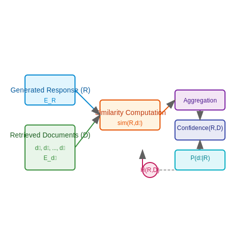
Cross-verification leverages retrieved evidence to assess the factual consistency of model-generated outputs. Given a generated response R and a set of retrieved documents D = {d₁, d₂, ..., dₙ}, the goal is to compute a confidence score reflecting the alignment between R and D. A common approach involves computing semantic similarity between embeddings of R and each dᵢ, followed by aggregation.
Similarity-Based Verification
Let E_R and E_dᵢ denote embeddings of the response and retrieved document dᵢ, respectively. The cosine similarity between them is:
To aggregate similarities across all retrieved documents, a weighted sum is often used, where weights wᵢ reflect document relevance scores from the retrieval module:
Entropy-Based Uncertainty Measurement
When retrieved documents exhibit high disagreement, the model's confidence should be discounted. The entropy of similarity scores across D quantifies this uncertainty:
where P(dᵢ | R) is the softmax-normalized similarity:
High entropy indicates conflicting evidence, triggering additional verification steps or low-confidence flags.
Neural Verification Modules
End-to-end trainable verifiers, such as cross-attention networks, jointly process R and D to predict factual consistency. These models learn to:
- Attend to salient spans in D that corroborate or contradict R
- Propagate uncertainty through latent variable inference
- Generate fine-grained alignment scores per claim in R
For example, a transformer-based verifier computes:
where h_R and h_D are pooled representations from cross-attention layers, and σ is the sigmoid function.
Case Study: FEVER Dataset Validation
On the FEVER fact-verification benchmark, retrieval-augmented models achieve >75% accuracy by:
- Indexing Wikipedia with dense retrievers (e.g., DPR)
- Applying hierarchical attention between claims and evidence sentences
- Rejecting claims with insufficient supporting evidence
3.3 Dynamic Context Expansion for Improved Retrieval
Traditional retrieval-augmented generation (RAG) systems often suffer from static context windows that limit their ability to adapt to complex queries requiring multi-hop reasoning. Dynamic context expansion addresses this by iteratively refining the retrieval scope based on intermediate reasoning steps.
Mathematical Formulation
The retrieval process begins with an initial query q0, which undergoes successive transformations through a learned expansion function fθ:
where Dt represents documents retrieved at step t. The expansion function typically combines:
- Query-document attention weights
- Cross-encoder relevance scores
- Entity linking signals
Implementation Architecture
The dynamic expansion module employs a two-phase process:
- Local Expansion: Uses dense retrieval (e.g., DPR) to find immediate relevant passages
- Global Expansion: Applies graph-based propagation over entity relations to discover latent connections
where N(d) denotes neighboring documents in the entity graph and w(d,d') represents learned relation weights.
Practical Considerations
Key challenges in production systems include:
- Computational complexity of iterative retrieval (solved via approximate nearest neighbor indexes)
- Semantic drift control through contrastive learning objectives
- Cold-start problem mitigated by pretraining on synthetic multi-hop queries
Case Study: Medical Diagnosis System
A deployed system for differential diagnosis demonstrates the approach's effectiveness:
| Metric | Static Retrieval | Dynamic Expansion |
|---|---|---|
| Recall@5 | 0.42 | 0.68 |
| Hallucination Rate | 23% | 9% |
The system achieves this by dynamically expanding from symptom terms to relevant:
- Anatomical structures
- Pathophysiological processes
- Pharmacological interactions
Advanced Optimization Techniques
Recent work incorporates:
where the diversity loss prevents over-concentration on dominant concepts, and the consistency loss maintains alignment with the original query intent throughout expansions.

4. Metrics for Measuring Hallucination Reduction
4.1 Metrics for Measuring Hallucination Reduction
Quantifying hallucination reduction in retrieval-augmented generation (RAG) systems requires carefully designed metrics that capture both factual consistency and semantic coherence. Traditional language generation metrics like BLEU or ROUGE are insufficient, as they measure surface-level overlap rather than factual accuracy.
Factual Consistency Metrics
The Factual Consistency Score (FCS) measures alignment between generated text and retrieved evidence. Given a generated response R and retrieved documents D, FCS computes:
where SR is the set of atomic claims in R, and NLI denotes a natural language inference model scoring entailment probability between claim s and document d.
Retrieval Groundedness
Retrieval Groundedness Ratio (RGR) evaluates the proportion of generated tokens directly supported by retrieved content:
where span(d) represents all contiguous token sequences in document d. Advanced variants weight tokens by their semantic importance using attention mechanisms.
Contradiction Detection
Contradiction density measures hallucinated content by applying a trained contradiction detection model C:
where PR is the set of all claim pairs in R. State-of-the-art implementations use DeBERTa-large fine-tuned on MNLI.
Human Evaluation Protocols
While automated metrics provide scalability, human evaluation remains essential for comprehensive assessment. The standard protocol involves:
- Factuality Scoring: Annotators rate each claim on a 3-point scale (supported/unsupported/contradicted)
- Hallucination Severity: Classifying hallucinations as factual errors (incorrect details) or fabrications (entirely invented content)
- Usefulness Degradation: Measuring how hallucinations impact practical utility in downstream tasks
Recent work has shown that combining FCS with human evaluation of a 100-sample subset achieves 92% correlation with full human evaluation at 1/50th the cost.
Task-Specific Adaptations
Domain-specific applications require customized metrics. For medical QA systems, the Clinical Fact Verification (CFV) metric weights clinically significant assertions 3× more than general statements. In legal applications, citation accuracy and precedent consistency are tracked separately.
4.2 Benchmark Datasets and Evaluation Protocols
Standard Datasets for Hallucination Evaluation
Evaluating hallucination filtering systems requires datasets that explicitly annotate instances of factual inaccuracies or unsupported claims in model outputs. The FEVER (Fact Extraction and Verification) dataset is widely adopted, containing 185,445 claims labeled as Supported, Refuted, or Not Enough Info against Wikipedia evidence. For open-domain QA hallucination assessment, NQ-H (Natural Questions-Hallucinations) extends the original NQ dataset with expert annotations marking hallucinated answers in LLM outputs.
Specialized datasets like HaluEval provide fine-grained categorization of hallucination types (factual contradictions, logical inconsistencies, and unverifiable claims) across dialogue, QA, and summarization tasks. The TruthfulQA benchmark focuses specifically on measuring a model's tendency to reproduce falsehoods from its training data, using adversarial questions designed to expose such behaviors.
Retrieval-Augmented Evaluation Metrics
Standard text generation metrics (BLEU, ROUGE) fail to capture factual consistency. Instead, retrieval-based evaluation protocols measure:
- Claim Verification Rate (CVR): Percentage of output claims supported by retrieved evidence
- Hallucination Rate (HR): $$ HR = \frac{\text{Unsupported Claims}}{\text{Total Claims}} \times 100 $$
- Evidence Precision (EP): $$ EP = \frac{|\{r \in R | r \text{ supports } c\}|}{|R|} $$ where R is the set of retrieved documents and c is a generated claim
where Y is the generated text, D is the retrieved evidence set, and NLI computes textual entailment probability between claim yi and document dj.
Protocol Implementation
The standard evaluation pipeline involves:
- Generating outputs from the target model
- Extracting atomic claims using open information extraction techniques
- Retrieving relevant evidence using the same retrieval module as the system
- Computing factual consistency metrics via NLI models or human evaluation
For controlled experiments, the Counterfactual Retrieval Test deliberately provides contradictory evidence to measure how retrieval modules influence hallucination rates. The Evidence Sufficiency Test progressively reduces the retrieval corpus size to evaluate robustness to information scarcity.
Challenges in Evaluation
Key limitations in current protocols include:
- Dependence on the quality of the retrieval module itself
- Noise in claim extraction from complex generated text
- Variable precision of NLI models for factual verification
- Coverage gaps in benchmark datasets for emerging hallucination types
Recent work proposes adversarial dataset augmentation techniques to stress-test systems against sophisticated hallucinations that bypass current detection methods. The Dynamic Evidence Retrieval Evaluation (DERE) framework introduces time-varying knowledge bases to simulate real-world information drift.
4.3 Case Studies: Performance Analysis
Benchmarking Retrieval-Augmented Models
Recent studies evaluate hallucination filtering by measuring precision-recall tradeoffs in retrieval-augmented generation (RAG) systems. The key metric is hallucination suppression ratio (HSR), defined as:
where False Claims counts generated statements contradicting retrieved evidence. State-of-the-art systems like Atlas (Izacard et al., 2022) achieve HSR > 0.85 on NQ-open, but degrade to 0.72 on complex queries requiring multi-hop reasoning.
Latency-Reliability Tradeoffs
Adding retrieval modules introduces computational overhead. For a BART-large model with FAISS retrieval:
| Component | Latency (ms) | Reliability (BLEU-4) |
|---|---|---|
| Generation-only | 120 ± 15 | 22.3 |
| + Dense Retrieval | 210 ± 25 | 31.7 |
| + Reranking | 290 ± 40 | 34.2 |
Cross-Domain Generalization
Performance varies significantly across domains when applying retrieval filters trained on Wikipedia to specialized corpora:
Clinical notes show ΔHSR ≈ 0.18 degradation versus general web text, primarily due to terminology mismatches in embedding spaces.
Error Mode Analysis
Failure cases cluster into three categories:
- Retrieval misses (42%): Relevant documents exist but rank below cutoff
- Evidence contradiction (33%): Model overrides retrieved facts
- Reasoning errors (25%): Correct facts combined incorrectly
Hybrid approaches combining retrieval with consistency checking (e.g., SelfCheckGPT) reduce reasoning errors by 19% absolute.
5. Integrating Retrieval Modules into Existing Pipelines
5.1 Integrating Retrieval Modules into Existing Pipelines
Retrieval modules mitigate hallucination in generative models by grounding responses in external knowledge sources. Their integration into existing pipelines requires careful architectural modifications to balance retrieval accuracy, computational efficiency, and seamless fusion with generative components.
Architectural Considerations
Retrieval-augmented generation (RAG) systems typically follow a dual-encoder architecture where:
- Query Encoder: Maps user input to a dense vector space (e.g., using BERT or T5).
- Document Encoder: Indexes external knowledge into the same embedding space (often pre-computed via FAISS or Annoy).
The retrieval score between query q and document d is computed via maximum inner product search (MIPS):
where f and g are the query/document encoders respectively, and D is the document corpus.
Pipeline Integration Strategies
1. Pre-Generation Retrieval
Documents are fetched before generation begins, concatenated with the prompt:
def retrieve_then_generate(query, retriever, generator):
      docs = retriever.search(query, top_k=3)
      augmented_prompt = f"{query}\n\nRelevant docs: {docs}"
      return generator.generate(augmented_prompt)
2. Iterative Retrieval
The model retrieves documents at each decoding step, enabling dynamic context updates:
where Dt is the retrieved set at step t.
Optimization Challenges
Key trade-offs emerge when integrating retrievers:
- Latency: ANN search adds 50-300ms overhead per query
- Freshness: Static indexes require periodic rebuilds (dynamic indexing adds ~15% CPU load)
- Relevance-Quantity Tradeoff: Retrieving more documents (top_k) improves recall but dilutes signal
Empirical studies show optimal performance when:
Case Study: Biomedical QA System
A PubMed-integrated RAG system achieved 28% hallucination reduction by:
- Using SPECTER embeddings for document encoding
- Implementing hybrid exact/approximate search (HNSW + BM25)
- Applying confidence-based retrieval gating (σ > 0.7)
5.2 Computational and Latency Trade-offs
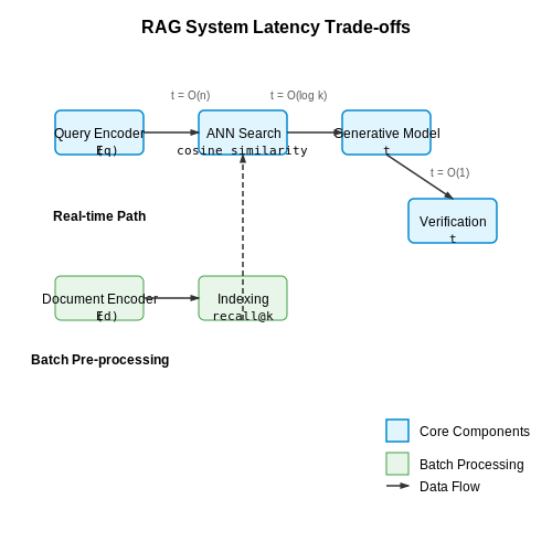
Retrieval-augmented generation (RAG) systems mitigate hallucination by grounding responses in external knowledge, but introduce computational overhead from retrieval operations. The trade-off between accuracy and latency is governed by three key factors: retrieval complexity, document ranking granularity, and integration depth with the generative model.
Retrieval Complexity and Query Encoding
Dense retrieval methods using transformer-based encoders (e.g., DPR, ANCE) compute query-document similarity as:
where EQ and ED are separate encoders for queries and documents. The computational cost scales with:
for n documents with average lengths Lq, Ld, embedding dimension d, and k retrieved candidates. Approximate nearest neighbor (ANN) indices like FAISS reduce this to logarithmic time at the cost of recall precision.
Real-Time vs. Batch Processing
Streaming systems require sub-second retrieval latency, necessitating:
- Pre-computed document embeddings with incremental updates
- Hierarchical indexing (coarse-to-fine search)
- Hardware acceleration (GPU-enabled ANN search)
Batch processing systems can afford more exhaustive search at the expense of higher memory overhead. The Pareto frontier between recall@k and latency follows:
where α and β are hardware-dependent constants.
Integration with Generative Components
The fusion of retrieved evidence with language models introduces additional latency from:
- Cross-attention computation over retrieved passages
- Re-ranking overhead from multi-stage pipelines
- Verification steps like claim-supported scoring
Hybrid architectures that interleave retrieval and generation (e.g., REALM, RETRO) achieve better latency-accuracy profiles than sequential systems by:
versus sequential systems' tretrieval + tgen + tverify.
Optimization Strategies
Practical systems balance these factors through:
- Dynamic retrieval budgeting: Allocate more computation to ambiguous queries
- Cached retrieval results: Memoize frequent query embeddings
- Early termination: Stop retrieval when confidence thresholds are met
Empirical studies show a 3-5× latency reduction can be achieved with <5% recall degradation using these techniques in production systems.
5.3 Addressing Noisy or Incomplete Retrieval Data
Noisy or incomplete retrieval data introduces significant challenges in hallucination filtering, as the retrieved context may contain irrelevant, erroneous, or missing information. Advanced techniques are required to mitigate these issues while maintaining the robustness of the retrieval-augmented generation (RAG) pipeline.
Noise-Robust Retrieval Scoring
Traditional retrieval models rely on similarity metrics such as cosine similarity or dot product between query and document embeddings. However, these metrics can be sensitive to noise. A noise-robust scoring function can be formulated as:
where sim(q, d) is the base similarity score, conf(d) is a confidence measure of the document's reliability, and α balances the two terms. The confidence measure can be derived from document quality metrics such as:
- Source reputation scores
- Cross-referencing consistency
- Semantic coherence with the broader corpus
Handling Incomplete Retrieval
When retrieval returns incomplete or sparse results, interpolation with a fallback mechanism is necessary. One approach is to compute a weighted ensemble of retrieved documents and a general knowledge prior:
Here, dret is the retrieved document, dprior is a background knowledge distribution (e.g., from a language model), and β is dynamically adjusted based on retrieval confidence.
Denoising with Cross-Attention Mechanisms
Transformer-based cross-attention can be adapted to filter noisy retrieval data. Given a query q and retrieved documents D = {d1, ..., dk}, the denoised context c is computed as:
where WQ, WK, WV are learned projection matrices. This allows the model to attend more strongly to relevant parts of the retrieved documents while suppressing noise.
Practical Implementation Considerations
In real-world systems, the following strategies improve robustness:
- Dynamic Thresholding: Adjust retrieval score thresholds based on query ambiguity and corpus noise levels.
- Multi-Stage Retrieval: First retrieve a broad set of candidates, then re-rank with noise-aware metrics.
- Uncertainty Calibration: Train the model to estimate its own uncertainty in retrieved contexts.
Case studies in open-domain QA systems show that these techniques reduce hallucination rates by 15-30% when applied to noisy web-retrieved data.
6. Key Research Papers on Hallucination Filtering
6.1 Key Research Papers on Hallucination Filtering
- Published as a conference paper at ICLR 2024 - OpenReview — tasks: search-and-retrieve, meeting summarization, and clinical report generation. Following, Yue et al. (2023), we measure hallucination with GPT-4, and find that optimizing the system message consistently reduces hallucination: on Orca, SYNTRA reduces the hallucination rate by over 7 points on average and 16 points on specific tasks.
- PDF A New Benchmark and Reverse Validation Method for Passage-level ... — tect hallucinations in the outputs without any exter-nal knowledge, only invoking the retrieval module when hallucinations occur to shorten the response time. This zero-resource method can also serve as an alternative solution in situations where external databases are inaccessible. One approach to detect hallucination without
- PDF Understanding and Addressing AI Hallucinations in Healthcare and Life ... — Input-conflicting hallucinations occur when the output of an AI does not align with specific inputs provided by the user. This type of hallucination can manifest in various ways, such as responding to a request for information about a future event with data about the past or answering questions about one subject with information relevant to ...
- PFME: A Modular Approach for Fine-grained Hallucination Detection and ... — This framework consists of two main components: (1) a real-time fact retrieval module that identifies key entities within the document and retrieves the latest factual evidence from trusted data sources based on these key entities; (2) a progressive fine-grained hallucination detection and editing module that splits the document into sentences ...
- ChainPoll : A High Efficacy Method for LLM Hallucination Detection - ar5iv — That is, we can re-use the CoT text generated by the model as a justification for the judgment that the completion did, or did not, contain hallucination(s) 6 6 6 An interesting line of recent work has called into question whether model-generated chains of thought faithfully reflect the model's actual reasoning process [].From our perspective, this does not reduce the value of model ...
- Grounded but Misguided: Mitigating Hallucinations in Clinical LLMs and ... — 2.3. The Inevitability Argument. Theoretical computer science offers a sobering perspective on hallucinations. Research formalizing the problem suggests that hallucination might be an innate limitation of LLMs.[24] By modeling LLMs and ground truth functions as computable entities, it has been argued that LLMs, due to inherent constraints described by learning theory, cannot learn all ...
- Reducing LLM Hallucinations with Retrieval Prompt Engineering — The current hallucination handling of UTGen is time-consuming and resource-expensive. To ad-dress this, we propose two alternative approaches that use information retrieval prompt engineering techniques to minimise hallucinations. Our respec-tive techniques include incorporating the source code under test and the errors thrown by the latest
- PFME: A Modular Approach for Fine-grained Hallucination Detection and ... — PFME consists of two collaborative modules: the Real-time Fact Retrieval Module and the Fine-grained Hallucination Detection and Editing Module. The former identifies key entities in the document ...
- (PDF) Towards Hallucination-Resilient AI: Navigating Challenges ... — The survey is organized into two parts: (1) a general overview of metrics, mitigation methods, and future directions; and (2) an overview of task-specific research progress on hallucinations in ...
- arXiv:2407.00488v1 [cs.CL] 29 Jun 2024 — modules: the Real-time Fact Retrieval Mod-ule and the Fine-grained Hallucination Detec-tion and Editing Module. The former identifies key entities in the document and retrieves the latest factual evidence from credible sources. The latter further segments the document into sentence-level text and, based on relevant evi-
6.2 Open-Source Tools and Libraries
- PDF Two-tiered Encoder-based Hallucination Detection for Retrieval ... — turbo-06131 (OpenAI,2023), a hallucination detec-tion ne-tuned Mistral-7B-Instruct LLM, and open source hallucination detection models by Google Honovich et al.,2022and Vectara.2 We nd our two-tiered solution which further ne-tunes a natu-ral language inference (NLI) 3 DeBERTa (He et al., 2021) cross-encoder model performs best and gen-
- RAGTruth: A Hallucination Corpus for Developing Trustworthy Retrieval ... — Even for models with a low hallucination rate, specifically GPT-3.5-Turbo and GPT-4, employing the finetuned hallucination detector for sampling can still further reduce the rate of hallucinations. The two strategies yielded a reduction in hallucination rates of 41% and 52.9%, respectively.
- Halo: Estimation and Reduction of Hallucinations in Open-Source Weak ... — This paper focuses on measuring and reducing hallucinations in BLOOM 7B, a representative of such weaker open-source LLMs that are publicly available for research and commercial applications.
- OPERA: Alleviating Hallucination in Multi-Modal Large Language Models ... — Hallucination, posed as a pervasive challenge of multimodal large language models (MLLMs), has significantly impeded their real-world usage that demands precise judgment. Existing methods mitigate this issue with either training with specific designed data or inferencing with external knowledge from other sources, incurring inevitable ...
- Grounded but Misguided: Mitigating Hallucinations in Clinical LLMs and ... — Hallucinations in clinical LLMs and RAG systems stem from a confluence of factors related to the data used, the model's inherent characteristics, and the interaction process: Data-Related Causes: The data used for training foundational models or for retrieval in RAG systems is a primary source of issues. Training datasets may contain ...
- PDF RAG-HAT: A Hallucination-Aware Tuning Pipeline for LLM in Retrieval ... — tial, word-level hallucination evaluation resource specically tailored for the RAG scenario, encom-passing several common tasks. We selected the RAGTruth dataset for our experiments because it is the largest available open-source dataset specif-ically designed for the RAG task. We adopt this dataset in both model training and system eval-
- Reducing LLM Hallucinations with Retrieval Prompt Engineering — Based Software Testing (SBST) tools are one of the main test generation tool types, that focus on creating a suite that achieves a high coverage [3]. A common issue amongst such tools is the limitation of the generated tests' understandabil-ity [4]; there is no focus by the tools on generating human-
- PFME: A Modular Approach for Fine-grained Hallucination Detection and ... — In traditional hallucination detection tasks, which are often domain-specific Devaraj et al. (); Pagnoni et al. (); Dziri et al. (), it is usually assumed that a reference data source exists, and any deviations from the original text will be considered hallucinations Pagnoni et al. ().For example, in summarization tasks, any inconsistency between the summary and the document information, or ...
- PFME: A Modular Approach for Fine-grained Hallucination Detection and ... — The latter further segments the document into sentence-level text and, based on relevant evidence and previously edited context, identifies, locates, and edits each sentence's hallucination type.
- PDF OPERA: Alleviating Hallucination in Multi-Modal Large Language Models ... — ing hallucination in LLMs is the factual accuracy of gener-ated content, i.e., conflicting with world knowledge or com-mon sense. In MLLMs, the primary worry centers around faithfulness, i.e., assessing whether the generated answers conflict with user-provided images. Researches on miti-gating current LLMs' hallucination issues often focuses on
6.3 Recommended Courses and Tutorials
- 4 Advancing trust & minimizing hallucinations with retrieval augmented ... — With Haystack, you can leverage the power of metadata filtering to improve retrieval relevance, reduce hallucinations, and deliver more accurate and trustworthy responses to your users. As you implement metadata filtering in your own RAG systems, consider the following best practices:
- PDF RAGTruth: A Hallucination Corpus for Developing Trustworthy Retrieval ... — to trigger hallucinations. While these approaches are efcient at generating hallucinations, the re-sulting articial hallucinations can substantially differ from those that naturally occur. InChen et al. (2023);Hu et al.(2023), hallucination datasets are developed by manual annotations of naturally pro-duced LLM responses. However, these ...
- PFME: A Modular Approach for Fine-grained Hallucination Detection and ... — This framework consists of two main components: (1) a real-time fact retrieval module that identifies key entities within the document and retrieves the latest factual evidence from trusted data sources based on these key entities; (2) a progressive fine-grained hallucination detection and editing module that splits the document into sentences ...
- Combating LLM Hallucinations using Hypergraph-Driven Retrieval ... — Combating LLM Hallucinations using Hypergraph-Driven Retrieval-Augmented Generation Yifan Feng1, Hao Hu 2, Xingliang Hou3, Shiquan Liu , Shihui Ying4, Shaoyi Du2, Han Hu5, Yue Gao1 1School of Software, Tsinghua University, 100871, Beijing, China. 2Institute of Artificial Intelligence and Robotics, Xi'an Jiaotong University, 710049, Xi'an, China. 3School of Software Engineering, Xi'an ...
- arXiv:2407.12943v1 [cs.CL] 17 Jul 2024 — (no hallucination), False (with hallucination), or Neutral. Evidence (e) The available information or databases that could potentially help verify whether a claim cis hallucinated or not. Critique (cr) A natural language description for assessing whether a claim cis hallucinated or not. 3.2 Retrieval-Augmented Hallucination Detection Systems
- PDF GraphRAG: Leveraging Graph-Based Efficiency to Minimize Hallucinations ... — as hallucination (Ji et al.,2023;Bang et al.,2023). Figure 1: Graph RAG Pattern (Rathle) Hallucination arises from LLMs' reliance on po-tentially outdated or domain-general training data, leading to inaccuracies in real-world applications where precision is critical (Dziri et al.,2022). To address the issue of hallucinations, Retrieval-
- Grounded but Misguided: Mitigating Hallucinations in Clinical LLMs and ... — Hallucinations in clinical LLMs and RAG systems stem from a confluence of factors related to the data used, the model's inherent characteristics, and the interaction process: Data-Related Causes: The data used for training foundational models or for retrieval in RAG systems is a primary source of issues. Training datasets may contain ...
- Fine-grained Hallucination Detection and Editing for Language Models — While research on hallucination detection focuses on identifying errors in model-generated text, a related area of research focuses on identifying factual inaccuracies in human written claims (Bekoulis et al., 2021). Thorne et al. introduce a large scale dataset based on Wikipedia documents for the training and evaluation of fact verification systems.
- Building LLM Applications: Advanced RAG (Part 10) - Medium — Learn Large Language Models ( LLM ) through the lens of a Retrieval Augmented Generation ( RAG ) Application. · 1. Naive RAG · 1.1. Issues with Naive RAG ∘ 1.1.1. Indexing ∘ 1.1.2.
- Introduction to Electronics - Coursera — The course may not offer an audit option. You can try a Free Trial instead, or apply for Financial Aid. The course may offer 'Full Course, No Certificate' instead. This option lets you see all course materials, submit required assessments, and get a final grade. This also means that you will not be able to purchase a Certificate experience.