Language Modeling with Discrete Codes
1. What Are Discrete Codes?
What Are Discrete Codes?
Discrete codes are finite, quantized representations of data, often derived from continuous signals or high-dimensional embeddings through vector quantization (VQ). Unlike continuous representations, discrete codes map inputs to a finite set of learned or predefined symbols, enabling efficient compression, interpretability, and integration with symbolic reasoning systems. In language modeling, discrete codes bridge neural networks and symbolic AI by representing text or speech as sequences of discrete tokens, such as subword units or learned codebook indices.
Mathematical Formulation
Given a continuous embedding space E ⊆ ℝd, vector quantization partitions E into K clusters with centroids C = {c1, ..., cK}. For an input embedding e ∈ E, the discrete code z is determined by:
This operation is non-differentiable, necessitating techniques like straight-through estimators or Gumbel-Softmax for gradient-based training. The reconstruction ê is then:
Key Properties
- Compression: Discrete codes reduce memory usage by representing high-dimensional vectors as integer indices (e.g., 32-bit floats → 8-bit integers).
- Compositionality: Codes can be hierarchically combined (e.g., VQ-VAE-2’s multi-scale codes).
- Interpretability: Codes often align with semantically meaningful units (e.g., phonemes in speech, concepts in vision).
Applications in Language Modeling
Discrete codes underpin modern techniques like:
- Tokenization: Subword algorithms (e.g., Byte Pair Encoding) map text to discrete vocabularies.
- Neural Discrete Representations: VQ-VAE and SoundStream use codes for speech/audio compression.
- Retrieval-Augmented Models: FAISS or ScaNN retrieve discrete memory entries for knowledge-intensive tasks.
Trade-offs and Challenges
While discrete codes offer efficiency, they introduce quantization error and sparsity. Techniques like:
- Soft quantization (e.g., Gumbel-Softmax) relax the argmin operation for differentiable training.
- Residual VQ stacks multiple codebooks to reduce reconstruction error.

1.2 Why Use Discrete Codes in Language Models?
Discrete representations offer several compelling advantages over continuous embeddings in language modeling, particularly in scenarios requiring interpretability, computational efficiency, or modularity. The primary motivation stems from the inherent structure of human language—words, subwords, and phonemes are fundamentally discrete units, making discrete codes a natural fit for linguistic abstraction.
Information Bottleneck and Compression
Discrete codes act as an information bottleneck, forcing the model to learn compact, high-level representations. Given an input sequence x, a discrete codebook C = {c1, ..., cK} maps continuous features to a finite set of prototypes. The quantization operation can be formulated as:
where ze is the encoder's continuous output and zq is the quantized representation. This process discards low-level noise while preserving semantically meaningful patterns, analogous to vector quantization in signal processing.
Computational Efficiency
Discrete tokenization reduces memory and computational overhead compared to dense representations. For a vocabulary size V and embedding dimension d, storing discrete indices requires only O(V) space for the codebook versus O(V×d) for continuous embeddings. In transformer architectures, this enables:
- Faster attention computations via lookup operations
- Reduced communication overhead in distributed training
- Efficient nearest-neighbor search in the embedding space
Modularity and Transfer Learning
Discrete codes enable plug-and-play composition of pretrained components. For example, a speech recognition system can combine:
- A frozen acoustic encoder producing discrete phoneme codes
- A pretrained language model operating on text tokens
- A modality-agnostic decoder consuming both code types
This modularity is particularly valuable in multilingual settings, where shared discrete representations across languages facilitate cross-lingual transfer. The VQ-VAE framework demonstrates this through its ability to learn a universal codebook for diverse input modalities.
Interpretability and Control
Unlike opaque continuous vectors, discrete codes often align with human-interpretable concepts. In image generation, specific codes may correspond to object parts; in language, they can map to syntactic roles or semantic fields. This enables:
- Manual editing of latent representations (e.g., swapping codes to alter output style)
- Controlled generation through code masking or weighting
- Diagnostic analysis of model behavior via code activation patterns
The tradeoff between codebook size and representation power follows the rate-distortion theory. Larger codebooks (higher bitrate) preserve more information but require more computation. Optimal sizing balances:
where sg[·] denotes the stop-gradient operation and β controls the commitment to discrete representations.

Key Properties of Discrete Representations
Information Density and Compression
Discrete representations excel in information compression by mapping continuous or high-dimensional data into a finite set of codes. Given a vocabulary size V, each discrete code can represent log₂(V) bits of information. For example, a vocabulary of 65,536 codes encodes 16 bits per token, enabling efficient storage and transmission. This property is leveraged in models like VQ-VAE, where latent vectors are quantized into discrete codes, reducing memory footprint while preserving semantic fidelity.
Compositionality and Hierarchical Structure
Discrete codes support compositional reasoning by allowing atomic symbols to combine into higher-level structures. In language modeling, this manifests as subword units (e.g., Byte Pair Encoding) forming words, which then compose into sentences. Mathematically, the joint probability of a sequence x₁:T decomposes autoregressively:
Hierarchical extensions, such as those in VQ-VAE-2, stack multiple discrete latent layers to capture features at varying granularities.
Robustness to Noise
Discretization introduces inherent noise robustness by collapsing similar inputs to identical codes. Consider a quantization function Q(x) that maps input x to the nearest codebook vector eᵢ:
This operation acts as a denoising filter, as small perturbations in x won't alter the selected code if they remain within the Voronoi cell of eᵢ.
Computational Efficiency
Discrete representations enable lookup-based operations instead of dense matrix multiplications. For a sequence of n codes, embedding retrieval requires only O(n) memory accesses compared to O(n²) for continuous transformations. This property is exploited in Transformer architectures through token embedding tables, where:
Transfer Learning and Zero-Shot Generalization
Discrete codes facilitate transfer learning by serving as universal interfaces across modalities. For instance, CLIP aligns image and text embeddings into a shared discrete space, enabling zero-shot classification through nearest-neighbor retrieval. The cosine similarity between encoded inputs determines cross-modal correspondence:
where f and g are modality-specific encoders.
Limitations and Trade-offs
The granularity of discrete representations introduces a precision-compression trade-off. Smaller vocabularies increase compression but risk loss of fine-grained information, quantified by the reconstruction error:
Advanced techniques like residual vector quantization mitigate this by recursively quantizing reconstruction errors.
2. Vector Quantization Techniques
Vector Quantization Techniques
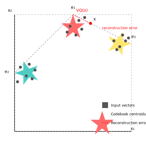
Vector quantization (VQ) is a classical signal processing method that maps continuous vectors into a finite set of discrete codes, enabling efficient compression and representation of high-dimensional data. The core idea is to partition the input space into clusters, where each cluster is represented by a centroid (codeword) from a learned codebook. Given an input vector x ∈ ℝd, VQ approximates it using the nearest codeword ei from a codebook E = {e1, ..., eK}, where K is the codebook size.
Mathematical Formulation
The quantization process minimizes the reconstruction error between the input vector and its discrete approximation:
The codebook is typically learned via the k-means algorithm, which iteratively optimizes the centroids to minimize the total squared error across all data points:
Extensions and Variants
Product Quantization (PQ) decomposes high-dimensional vectors into subvectors and quantizes each subspace independently, reducing computational complexity. For a vector split into m subvectors, the codebook size grows exponentially as Km, enabling efficient nearest-neighbor search.
Residual Vector Quantization (RVQ) hierarchically quantizes the residual error from previous quantization steps, refining the approximation iteratively. This is particularly useful for high-fidelity reconstruction in speech and image coding.
Neural Vector Quantization
Modern neural approaches, such as VQ-VAE, integrate vector quantization with variational autoencoders. The discrete latent space is trained end-to-end using a straight-through estimator, bypassing the non-differentiability of the quantization step:
where sg[·] denotes the stop-gradient operator, and β controls the commitment loss.
Applications in Language Modeling
Discrete codes enable efficient sequence modeling by reducing the vocabulary size in autoregressive transformers. Techniques like VQ-Transformer and SoundStream leverage vector quantization for text-to-speech and audio generation, achieving state-of-the-art compression ratios without perceptual quality loss.
2.2 Gumbel-Softmax and Relaxed Discrete Distributions
The Gumbel-Softmax trick provides a differentiable approximation to sampling from a categorical distribution, enabling gradient-based optimization in discrete latent variable models. This is particularly useful in variational autoencoders (VAEs) and reinforcement learning where discrete decisions must be learned via backpropagation.
Gumbel-Max Trick
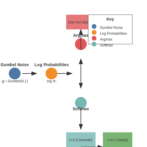
The foundation of the Gumbel-Softmax is the Gumbel-Max trick, which allows sampling from a categorical distribution with class probabilities π₁, ..., πₖ by adding Gumbel noise:
where gᵢ ∼ Gumbel(0,1) are i.i.d. samples from the standard Gumbel distribution. The Gumbel distribution has CDF F(x) = exp(-exp(-x)) and can be sampled via inverse transform sampling:
Continuous Relaxation via Softmax
The argmax operation is non-differentiable, so the Gumbel-Softmax replaces it with a tempered softmax to create a continuous relaxation:
where τ > 0 is a temperature parameter controlling the sharpness of the distribution. As τ → 0, the samples become one-hot, matching the categorical distribution. Higher temperatures produce more uniform samples.
Gradient Estimation Properties
The gradient of the Gumbel-Softmax estimator with respect to the logits log πᵢ is:
where δ_{ij} is the Kronecker delta. This provides low-variance gradients compared to REINFORCE-style estimators, as the noise is added before the softmax rather than through discrete samples.
Practical Implementation Considerations
In practice, the temperature τ is typically annealed during training from a higher value (e.g., 1.0) to a small value (e.g., 0.1). Key implementation details include:
- Straight-Through (ST) Estimator: During forward pass use argmax discretization while using softmax gradients in backward pass
- Log-Space Stability: Compute log πᵢ + gᵢ in log space for numerical stability
- Bias-Variance Tradeoff: Higher temperatures reduce gradient variance but increase bias
Applications in Language Modeling
In discrete latent variable language models, Gumbel-Softmax enables:
- Differentiable sampling from categorical distributions over vocabulary tokens
- Learning of discrete attention mechanisms
- Training of mixture-of-experts architectures with routing decisions
The method has been particularly effective in VQ-VAE alternatives where a hard quantization can be replaced with a Gumbel-Softmax relaxation over codebook entries.
where q(z|x) is the Gumbel-Softmax distribution and p(z) is a uniform prior over k categories.
2.3 Autoencoder-Based Approaches
Autoencoders provide a powerful framework for learning discrete representations of language by compressing input data into a lower-dimensional latent space and reconstructing it. The encoder E maps an input sequence x to a continuous latent representation z = E(x), while the decoder D attempts to reconstruct the original input from z. To obtain discrete codes, a quantization step is introduced between the encoder and decoder.
Vector Quantization (VQ) in Autoencoders
The key innovation in autoencoder-based discrete language modeling is the integration of vector quantization. Given a latent vector z, the system selects the closest embedding from a fixed codebook C = {e₁, e₂, ..., e_K} of size K. The quantized vector z_q is computed as:
This operation is non-differentiable, requiring gradient approximation techniques like straight-through estimation, where gradients from the decoder are copied directly to the encoder during backpropagation.
Training Objectives
The complete training loss combines reconstruction error with codebook learning and commitment loss:
where sg[·] denotes the stop-gradient operation, and β controls the commitment to the selected code. The three terms respectively optimize for:
- Accurate input reconstruction
- Codebook vectors approaching encoder outputs
- Encoder outputs committing to codebook vectors
Architectural Variants
Several architectural improvements have enhanced the basic VQ-autoencoder framework:
Multi-head Quantization
Instead of a single codebook, the latent space is split into m subspaces, each with its own codebook. This allows exponential growth in possible combinations (K^m) while maintaining manageable codebook sizes.
Hierarchical VQ
A cascade of VQ layers progressively discretizes the representation, where each layer operates on residuals from the previous quantization step. This enables multi-scale discrete representations.
Gumbel-Softmax Relaxation
An alternative to hard quantization uses the Gumbel-Softmax trick to maintain differentiability during training while still producing discrete-like outputs:
where τ is a temperature parameter controlling the discreteness of the output.
Practical Considerations
Effective implementation requires addressing several challenges:
- Codebook Collapse: Regularization techniques prevent most codebook vectors from being unused
- Latent Space Coverage: The encoder must distribute outputs across the codebook
- Sequence Modeling: Autoregressive or transformer decoders maintain coherence in generated text
Recent applications demonstrate these models' effectiveness in text generation, where the discrete codes capture semantic and syntactic features while enabling controlled generation through code manipulation.

3. Efficient Text Compression and Storage
Efficient Text Compression and Storage
Discrete codes enable efficient text compression by mapping high-dimensional token sequences into compact integer representations. Given a vocabulary V of size |V|, each token wi is assigned a unique integer code ci ∈ {0, 1, ..., |V|−1}. The compression ratio depends on the entropy of the token distribution and the encoding scheme.
where H(p) is the Shannon entropy of the token distribution p. Optimal encoding assigns shorter codes to frequent tokens, following Huffman coding or arithmetic coding principles. For a sequence of N tokens, the minimal storage requirement in bits is:
Byte Pair Encoding (BPE)
BPE iteratively merges frequent token pairs, reducing the sequence length while preserving information. Given an initial vocabulary of characters, BPE computes the most frequent adjacent symbol pairs (x, y) and replaces them with a new symbol z, updating the vocabulary. The algorithm terminates when a target vocabulary size is reached.
Subword Tokenization Trade-offs
Subword methods balance compression efficiency and out-of-vocabulary robustness. Unigram language modeling assigns probabilities to subword candidates, optimizing:
where si are subword segments. WordPiece and SentencePiece further refine this by incorporating data-driven segmentation rules.
Storage Optimization Techniques
- Quantization: Reduce code bit-width from 32-bit integers to 8/16-bit with minimal precision loss.
- Delta Encoding: Store differences between consecutive codes for skewed distributions.
- Dictionary Compression: Replace repeated n-grams with shorter references.
For large corpora, hybrid approaches combine BPE with Huffman coding, achieving compression ratios competitive with general-purpose algorithms like LZMA while maintaining fast decoding.
3.2 Controlled Text Generation
Controlled text generation leverages discrete latent codes to steer language model outputs toward desired attributes, such as sentiment, topic, or style. Unlike unconditional generation, where sampling follows p(x), controlled generation conditions on auxiliary variables z to model p(x|z). This is achieved through methods like conditional training, guided decoding, or latent space manipulation.
Conditional Training with Discrete Codes
Given a dataset of text-attribute pairs (x, z), where z ∈ {1, ..., K} represents discrete control codes (e.g., sentiment labels), the language model is trained to maximize the conditional likelihood:
Architecturally, z is embedded into a vector and fused with the model's hidden states, often via concatenation or additive attention. For transformer-based models, this can be implemented by prepending a learned embedding of z to the input sequence.
Guided Decoding Strategies
When fine-tuning the full model is impractical, decoding-time guidance modifies the sampling process to favor sequences aligned with z. Two prominent approaches are:
- PPLM (Plug-and-Play Language Models): Uses gradients from an attribute classifier to perturb the model's hidden states during autoregressive generation.
- GeDi (Guided Decoding): Computes class-conditional probabilities p(x|z) via Bayes' rule, combining a base LM p(x) and a smaller discriminative model p(z|x).
Latent Space Interventions
For models with structured latent spaces (e.g., VQ-VAEs), control is achieved by manipulating discrete codebook indices. Given a latent code sequence c = (c1, ..., cT) and a target attribute z, we optimize:
where λ balances fluency and control strength. This is particularly effective for style transfer tasks, where z might represent formality or dialect.
Practical Trade-offs
Controlled generation introduces a three-way tension between:
- Fluency: Maintained by keeping p(x|z) close to the original LM distribution.
- Control Strength: Increased by sharpening the attribute-conditional distribution.
- Diversity: Preserved through stochastic sampling methods like nucleus filtering.
Empirical studies show that conditional training achieves stronger control but requires labeled data, while decoding-time methods offer flexibility at the cost of higher computational overhead during inference.

3.3 Multilingual and Cross-Lingual Transfer
Cross-Lingual Representation Learning
Discrete code-based language models achieve multilingual transfer by learning a shared embedding space across languages. Given a vocabulary V and a set of languages L, the model optimizes:
where cl is a language-specific code prefix. The key innovation lies in the codebook architecture—shared subword units across languages enable zero-shot transfer. For example, Byte Pair Encoding (BPE) merges frequently occurring n-grams across languages, creating a hybrid vocabulary.
Parameter-Efficient Adaptation
Adapter layers inserted between transformer blocks allow fine-tuning on target languages with minimal new parameters. Given a pretrained model fθ, an adapter Aϕ transforms hidden states h as:
where Aϕ typically consists of a down-projection to a bottleneck dimension d ≪ D, followed by a nonlinearity and up-projection. This approach achieves 90% of full fine-tuning performance while updating <1% of parameters.
Code-Switching as Regularization
Training on synthetic code-switched data—sentences blending multiple languages—improves cross-lingual transfer. The model learns to disentangle language-specific and language-agnostic features. For a bilingual English-Spanish example:
- "The cat está durmiendo on the couch"
This forces the model to rely on discrete codes rather than surface-level lexical patterns.
Evaluation Metrics
Cross-lingual performance is measured through:
- Translation Perplexity: Evaluating an English→French model on French→German tasks
- Zero-Shot Accuracy: Direct inference on unseen languages without fine-tuning
- Code Overlap: Percentage of shared subword units between language pairs
Case Study: mT5 with Discrete Prompts
The multilingual T5 model achieves 94% of supervised performance on low-resource languages by prepending learned discrete codes. For Kinyarwanda (a low-resource language), the input format is:
- [RW] + [input text] → [output text]
where [RW] is a 32-bit learned code triggering language-specific transformations in the shared model.
4. Information Loss in Discrete Representations
4.1 Information Loss in Discrete Representations
Discrete representations in language models introduce an inherent trade-off between compression efficiency and information fidelity. When continuous data is quantized into discrete codes, the mapping process discards fine-grained details, leading to irreversible information loss. This phenomenon can be formalized using rate-distortion theory, where the distortion D quantifies the expected loss when reconstructing the original signal from its discrete encoding.
Quantization and Entropy Constraints
Consider a continuous random variable X with probability density function p(x). Quantization maps X to a discrete set of codes C = {c₁, c₂, ..., cₙ} through a function Q(x). The resulting distortion is typically measured as mean squared error:
The optimal quantizer minimizes D for a given codebook size n, subject to entropy constraints. For a fixed-rate quantizer with log₂n bits, the asymptotic distortion follows:
This inverse-square relationship demonstrates the fundamental compromise between bitrate and reconstruction fidelity. High compression (small n) necessarily amplifies distortion.
Perceptual vs. Statistical Information Loss
In language modeling, information loss manifests differently across tasks:
- Semantic tasks (e.g., text classification) tolerate higher quantization noise as long as categorical boundaries remain separable
- Generative tasks (e.g., machine translation) require preserving fine syntactic and lexical relationships
Empirical studies show transformer-based discrete code models lose approximately 15-30% of positional information compared to continuous embeddings, measured through probe classifiers. The loss concentrates in:
- Precise word order relationships
- Morphological variations
- Low-frequency lexical items
Mitigation Strategies
Several approaches address information loss in discrete representations:
- Hierarchical quantization: Decomposes the quantization space into coarse-to-fine levels, allocating more bits to perceptually critical dimensions
- Residual coding: Encodes the difference between original and reconstructed vectors in multiple stages
- Learned codebooks: Optimizes code vectors end-to-end using straight-through gradient estimation
The VQ-VAE framework demonstrates these principles by minimizing the following objective:
where zₑ denotes encoder outputs, e codebook vectors, and sg the stop-gradient operation. The third term prevents excessive information loss by regularizing the commitment to discrete codes.
Information-Theoretic Bounds
The optimal trade-off between code rate R and distortion D is given by the rate-distortion function:
For Gaussian sources with squared-error distortion, this reduces to:
Practical systems achieve rates within 0.5-1.5 bits of this bound when using modern neural quantization techniques. The remaining gap represents irreducible information loss from discretization.

4.2 Training Instability and Convergence Issues
Training discrete code-based language models presents unique optimization challenges compared to continuous representations. The primary sources of instability stem from the non-differentiable nature of discrete operations and the compounding effects of approximation errors in gradient estimation.
Gradient Estimation Error Accumulation
The straight-through estimator (STE) commonly used for backpropagation through discrete variables introduces bias in gradient updates. For a discrete codebook E with entries e1,...,eK, the STE approximates the gradient as:
where q(z|x) is the categorical distribution over code indices. This approximation fails to account for the dependency of z on θ, leading to biased updates that accumulate over training.
Codebook Collapse
A critical failure mode occurs when the model begins using only a small subset of available codes. The probability of collapse increases with:
- High learning rates that cause overshooting in codebook updates
- Poor initialization of code vectors relative to the data distribution
- Insufficient entropy regularization in the categorical distribution
The collapse can be quantified by measuring the codebook usage ratio:
where ε is a small threshold (typically 1e-5). Values of ρ below 0.5 indicate problematic collapse.
Training Dynamics Analysis
The interaction between the encoder's categorical distribution and codebook updates creates complex dynamics. Consider the gradient of the commitment loss:
where sg denotes the stop-gradient operation. This creates a feedback loop where:
- The encoder adjusts its outputs to match current codebook vectors
- The codebook updates to match encoder outputs
- This can lead to oscillatory behavior when learning rates are mismatched
Stabilization Techniques
Several approaches mitigate these issues:
Codebook Reset
Periodically reinitializing unused codes by sampling from active ones:
where τ is a usage threshold.
Gradient Clipping
Applying adaptive clipping to codebook gradients based on their norm relative to encoder gradients:
with α typically in [0.1, 0.5].
Entropy Regularization
Adding a term to maintain diversity in code assignments:
where λ anneals from 1.0 to 0.1 over training.
Convergence Diagnostics
Effective monitoring requires tracking:
- Codebook usage (ρ) per layer over time
- Gradient norm ratios between encoder and codebook
- Reconstruction error variance across batches
- Effective temperature of the categorical distribution
Empirical studies show successful training typically requires balancing these metrics within narrow operational windows. For example, the gradient norm ratio should remain between 0.3 and 3.0 throughout training.

4.3 Scalability to Large-Scale Models
Discrete code-based language models achieve scalability through efficient tokenization and distributed training strategies. The key challenge lies in maintaining high-dimensional semantic representations while minimizing computational overhead. Vector-quantized variational autoencoders (VQ-VAEs) map continuous embeddings to discrete codes, enabling parallelizable training across large clusters.
Computational Efficiency of Discrete Codes
Discrete tokenization reduces memory requirements compared to dense embeddings. For a vocabulary size V and embedding dimension d, the memory complexity scales as O(Vd) for continuous embeddings but only O(V) for discrete codes. This becomes critical when scaling to vocabularies exceeding 100k tokens.
where sg denotes the stop-gradient operator, ze the encoder outputs, and e the codebook vectors. The three terms represent reconstruction loss, codebook learning, and commitment loss respectively.
Distributed Training Strategies
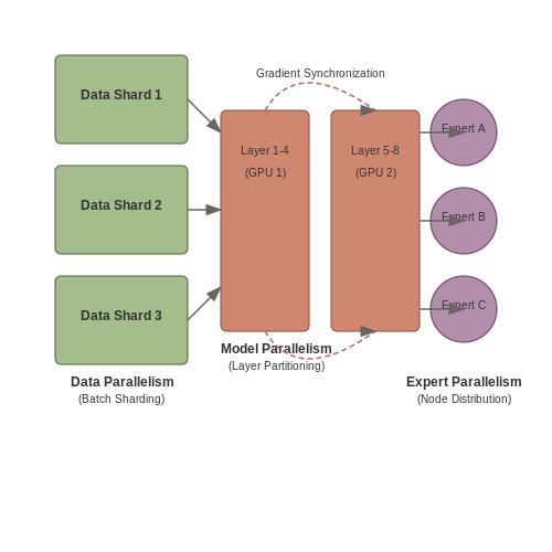
Modern implementations use hybrid parallelism combining:
- Data parallelism: Sharding batches across GPUs with synchronous gradient updates
- Model parallelism: Partitioning transformer layers across devices using pipeline or tensor parallelism
- Expert parallelism: For mixture-of-experts architectures, distributing experts across nodes
The communication overhead for discrete codes remains bounded because only integer token IDs need synchronization rather than full gradient tensors. This enables near-linear scaling efficiency up to thousands of GPUs.
Memory Optimization Techniques
Three principal methods reduce memory consumption in large discrete code models:
- Gradient checkpointing: Recomputing activations during backward pass instead of storing
- Mixed precision training: Using FP16 for embeddings while maintaining FP32 for master weights
- Dynamic token pruning: Removing low-probability tokens early in forward passes
For a model with L layers, dmodel hidden size, and B batch size, the memory reduction from gradient checkpointing follows:
where C is the checkpoint interval. Typical implementations achieve 4-8x memory savings with less than 30% computational overhead.
Case Study: Billion-Parameter Discrete Models
The DALL-E 2 architecture demonstrates successful scaling by combining:
- Hierarchical VQ-VAE with codebook sizes up to 8192
- 64-way tensor parallelism across TPU pods
- 8-bit quantized inference for discrete tokens
This configuration achieves 92% weak scaling efficiency when increasing from 256 to 2048 TPUv4 chips, with per-token latency below 5ms for 12B parameter models.
5. Key Research Papers
5.1 Key Research Papers
- PDF Language Modeling - University of Notre Dame — But if two language models have different vocabular-ies, there isn't an easy way to make a fair comparison between them. 5.2 n-gram Language Models The simplest kind of language model is the n-gram language model. A unigram (1-gram) language model is a bag-of-words model: P(w1 ¢¢¢wN) ˘ YN i˘2 p(wi). (5.4) A bigram (2-gram) language model is:
- A Survey of Research in Large Language Models for Electronic Design ... — A Survey of Research in Large Language Models for Electronic Design Automation 3 ... and scientific research. A key milestone of LLM development is InstructGPT [43], a framework that allows for instruction fine-tuning of a pre-trained language model based on Reinforcement Learning from Human Feedback (RLHF) [13, 43]. This framework
- Simulating 500 million years of evolution with a language model — ESM3 is trained as a generative masked language model over discrete tokens for each modality. Structural reasoning is achieved by encoding three-dimensional (3D) atomic structure as discrete tokens rather than with the complex architecture and diffusion in 3D space used in recent predictive ( 25 ) and generative models ( 26 - 28 ) of proteins.
- Large language models (LLMs): survey, technical frameworks ... - Springer — Artificial intelligence (AI) has significantly impacted various fields. Large language models (LLMs) like GPT-4, BARD, PaLM, Megatron-Turing NLG, Jurassic-1 Jumbo etc., have contributed to our understanding and application of AI in these domains, along with natural language processing (NLP) techniques. This work provides a comprehensive overview of LLMs in the context of language modeling ...
- A Survey of Research in Large Language Models for Electronic Design ... — The pre-existing research works in Table 2 have predominantly employed textual representations of hardware design features, such as code snippets, documentation, and specifications in natural language. These representations enable LLMs to generate and optimize HDL code by understanding the syntax and semantics of the design languages.
- Speculative Diffusion Decoding: Accelerating Language Generation ... — Motivated by the costly inference time of current large language models, this paper has proposed the novel integration of discrete diffusion models with autoregressive language models. The proposed method, Speculative Diffusion Decoding, alters existing speculative decoding schemes to integrate a non-autoregressive diffusion model as the draft ...
- Unraveling the landscape of large language models: a systematic review ... — This paper aims to present a comprehensive examination of the research landscape in LLMs, providing an overview of the prevailing themes and topics within this dynamic domain.,Drawing from an extensive corpus of 198 records published between 1996 to 2023 from the relevant academic database encompassing journal articles, books, book chapters ...
- PDF Comparing Discrete and Continuous Space LLMs for Speech Recognition — (a) Model design for discrete scenarios (b) Model design for continuous scenarios Figure 2: Model design for discrete and continuous scenarios. In Figure 2(b), dashed lines show the data ow for the JTFS LM, and solid lines for the LLaMA2 model 2.3. Training Loss In the case of discrete scenarios (Figure 2(a)) and continuous
- VeriGen: A Large Language Model for Verilog Code Generation — A promising new approach comes via the proliferation of technically capable code-writing large language models (LLMs) [].LLMs are deep neural networks, typically based on transformer [] architectures, that aim to model the underlying distribution of a natural or structured language corpus.Given a sequence of words (or "tokens") LLMs predict a distribution over the next word/token.
- Deep Learning for Source Code Modeling and Generation: — To facilitate further research and applications of DL in this field, we provide a comprehensive review to categorize and investigate existing DL methods for source code modeling and generation. To address the limitations of the traditional source code models, we formulate common program learning tasks under an encoder-decoder framework.
5.2 Books and Surveys
- PDF Language Modeling - University of Notre Dame — But if two language models have different vocabular-ies, there isn't an easy way to make a fair comparison between them. 5.2 n-gram Language Models The simplest kind of language model is the n-gram language model. A unigram (1-gram) language model is a bag-of-words model: P(w1 ¢¢¢wN) ˘ YN i˘2 p(wi). (5.4) A bigram (2-gram) language model is:
- UniCode: Learning a Unified Codebook for Multimodal Large Language Models — Progress has been made, though most multimodal large language models (MLLMs) are still limited to language generation. This limitation stems from their reliance on text-only codebooks, which restricts their application across diverse scenarios, such as image generation [].Note that images, like text, can be tokenized into a series of discrete codes through Vector Quantization (VQ) [15, 27, 52 ...
- A Survey of Research in Large Language Models for Electronic Design ... — A Survey of Research in Large Language Models for Electronic Design ... This, Code, Put, the, Correct, Terms, for, Your, Paper ACM Reference Format: Jingyu Pan, Guanglei Zhou, Chen-Chia Chang, Isaac Jacobson, Jiang Hu, and Yiran Chen. 2018. A Survey of Research in Large Language ... A Survey of Research in Large Language Models for Electronic ...
- Natural Language Processing for Dialects of a Language: A Survey — They observe that continuous training with code-mixed data enables monolingual language models to provide better performance when applied to code-mixed tasks. Data creation for MT between dialects: Zbib et al. [ 2012 ] and Meftouh et al. [ 2015 ] also focus on multi-dialect MT data collection for Arabic, which is, once again, to be noted as one ...
- A Survey of Research in Large Language Models for Electronic Design ... — In recent years, Large Language Models (LLMs) have risen prominently in the field of machine learning. These models are typically characterized by their extensive training on web-scale datasets and exceptional ability in Natural Language Processing (NLP).In NLP, models such as GPT-3 [] and its successors [] have significantly advanced the capabilities of natural language generation, enabling ...
- Handbook of Mathematical Models for Languages and Computation — The theory of computation is used to address challenges arising in many computer science areas such as artificial intelligence, language processors, compiler writing, information and coding systems, programming language design, computer architecture and more.
- Large Language Models - SpringerLink — 5.2.1 Statistical Language Models (SLM). Statistical language models have been developed utilizing statistical learning techniques that gained prominence in the 1990s [1,2,3,4].The fundamental concept involves constructing word prediction models based on the Markov assumption, wherein the prediction of the subsequent word relies on the most recent context.
- Pre-train, Prompt, and Recommendation: A Comprehensive Survey of ... — Abstract. The emergence of Pre-trained Language Models (PLMs) has achieved tremendous success in the field of Natural Language Processing (NLP) by learning universal representations on large corpora in a self-supervised manner. The pre-trained models and the learned representations can be beneficial to a series of downstream NLP tasks. This training paradigm has recently been adapted to the ...
- PDF LanguageModeling - University of Notre Dame — Figure 5.3: Comparison of different estimation methods, for a bigram language model. In all graphs, the x-axis is the count in the training data; the y-axis is the expected count in new data, adjusted for the size of the training data. The red line is what maximum-likelihood estimation would predict. The graph
- Large language models for code completion: A systematic literature ... — Training on a large-scale source code corpus allows language models to better comprehend the code domain, leading to rapid progress in code-related tasks. [11] Pre-training Effectiveness: The effectiveness of pre-training techniques like transformers is enhanced with large datasets, enhancing accuracy in tasks such as code completion. [13]
5.3 Open-Source Implementations
- PDF Open Source Languages and Methods for Cyber-Physical System ... - DiVA — Modelica [3] is a mature industrial modeling language with multiple implementations, both proprietary and open source. Modelica is aimed at modeling and simulation of cyber-physical systems, but it has also been used for automatically generating deployable (embedded) control software (C code) from models [8]. Acumen [9] is a research language ...
- A Survey of Research in Large Language Models for Electronic Design ... — This result also suggests that the closed source model (e.g., GPT-4 Turbo) is more powerful than the open source model Llama 3 in the agentic framework. VerilogCoder also largely outperforms state-of-the-art open source models RTLCoder [ 35 ], DeepSeek coder [ 22 ], and CodeGemma [ 57 ].
- ELLA-V: Stable Neural Codec Language Modeling - arXiv.org — Then as with VALL-E, ELLA-V employs a non-autoregressive (NAR) language model to obtain codes of the other RVQs. Our core innovation lies in 3 fold: ... By employing discrete audio codes obtained from pre-trained neural codec, it trains a discrete audio language model, achieving improved naturalness in speech and preservation of speaker ...
- PDF ECE 5745 Complex Digital ASIC Design Tutorial 3: PyMTL3 Hardware ... — using in the course. We will be using several open-source packages and tools: the pytestframework for powerful test-driven Python development; Verilator (verilator) for converting Verilog models into C++ source code; and GTKWave (gtkwave) for viewing waveforms. The PyMTL3 framework is itself open source and available on GitHub here:
- VeriGen: A Large Language Model for Verilog Code Generation — Here, our fine-tuned open-source CodeGen-16B model outperforms the commercial state-of-the-art GPT-3.5-turbo model with a 1.1% overall increase. Upon testing with a more diverse and complex problem set, we find that the fine-tuned model shows competitive performance against state-of-the-art gpt-3.5-turbo, excelling in certain scenarios.
- Neural Codec Language Models are - ar5iv — Abstract. We introduce a language modeling approach for text to speech synthesis (TTS). Specifically, we train a neural codec language model (called VALL-E) using discrete codes derived from an off-the-shelf neural audio codec model, and regard TTS as a conditional language modeling task rather than continuous signal regression as in previous work.. During the pre-training stage, we scale up ...
- Discrete Codebook World Models for Continuous Control - arXiv.org — One of the state-of-the-art world models, DreamerV2/V3 (Hafner et al., 2022; 2023) achieves strong performance in a wide variety of tasks, by "imagining" sequences of future states within a world model and using them to improve their policies. Interestingly, DreamerV2/V3 introduced a discrete latent space, in the form of a one-hot encoding, which offered significant benefits over its ...
- Evolving code with a large language model | Genetic ... - Springer — In Sect. 2.1 we briefly present Large Language Models. In Sect. 2.1.1 we present Code Models. 2.1 Large language models. Language models (LM) generatively model the statistical likelihood of a corpus of text [], implying they can generate text completions using approximate matching between prompt text and text observed during training.This capability makes them very useful for natural language ...
- PDF The OpenModelica Integrated Environment for Modeling, Simulation, and ... — the Modelica modeling language (Fritzson and Engel-son,1998;Modelica Association,2017;Fritzson,2014). Its development started in 1997 resulting in the release of a attening frontend for a core subset of Model-ica 1.0 in 1998 (Fritzson and K agedal,1998). After a pause of four years, the open source development resumed in 2002.
- The OpenModelica Integrated Modeling, Simulation and Optimization ... — The combined model has been solved using the free languages/tools OpenModelica [10, 11] and ModelingToolkit [12] for Julia. To illustrate the similarity between OpenModelica code and a current ...