Masked Language Modeling Explained
1. Definition and Core Concepts
Masked Language Modeling: Definition and Core Concepts
Masked language modeling (MLM) is a self-supervised pre-training objective in natural language processing (NLP) where a model learns to predict randomly masked tokens in a sequence based on their bidirectional context. Unlike autoregressive models that predict tokens sequentially (left-to-right or right-to-left), MLM enables full-context understanding by conditioning predictions on both preceding and succeeding tokens.
Mathematical Formulation
Given an input sequence X = (x1, ..., xn), MLM randomly replaces a subset of tokens with a special [MASK] token, producing a corrupted version X̃. The model then learns to reconstruct the original sequence by predicting the masked tokens x̃m conditioned on the entire corrupted sequence:
where hm is the hidden representation of the masked position, and W, b are learnable parameters. The training objective maximizes the log-likelihood of the correct tokens:
where M is the set of masked positions.
Key Architectural Features
- Bidirectional Context: Unlike unidirectional models, MLM leverages both left and right contexts for predictions, enabling deeper linguistic understanding.
- Dynamic Masking: Modern implementations (e.g., BERT) apply masking dynamically during training, where different tokens are masked in different epochs, improving robustness.
- Partial Masking Strategy: Typically, 15% of tokens are masked, with variations: 80% replaced by [MASK], 10% by random tokens, and 10% left unchanged to balance noise and learning signal.
Practical Considerations
MLM's effectiveness stems from its ability to learn rich contextual representations without labeled data. However, the discrepancy between pre-training (where [MASK] tokens are present) and fine-tuning (where they are absent) creates a pretrain-finetune mismatch. Solutions include:
- Using replacement tokens during fine-tuning to simulate masked contexts
- Employing techniques like whole-word masking or span masking to better align with downstream tasks
The computational cost scales quadratically with sequence length due to the self-attention mechanism in transformer architectures, making long-sequence MLM challenging without optimizations like sparse attention or memory-efficient variants.
Historical Context and Evolution
The development of masked language modeling (MLM) traces its roots to early probabilistic language models, but its modern incarnation emerged from advancements in neural networks and self-supervised learning. The concept of predicting missing or obscured tokens in a sequence was first explored in noise-contrastive estimation and denoising autoencoders, where models were trained to reconstruct corrupted inputs. However, the breakthrough came with the introduction of the Transformer architecture in 2017, which enabled efficient parallel processing of sequential data and scaled self-attention mechanisms.
Early Predecessors: From n-grams to Neural LMs
Before MLM, statistical language models like n-grams and hidden Markov models (HMMs) dominated, relying on fixed-window co-occurrence statistics. Neural language models, such as word2vec and GloVe, improved contextual representation but still operated on shallow architectures. The shift to deep learning introduced recurrent neural networks (RNNs) and long short-term memory (LSTM) networks, which handled variable-length sequences but suffered from vanishing gradients and sequential computation bottlenecks.
This n-gram probability formulation highlights the limitations of count-based methods, which fail to capture long-range dependencies or generalize to unseen sequences.
The Transformer Revolution
The 2017 paper "Attention Is All You Need" introduced the Transformer, replacing recurrence with self-attention:
where Q, K, and V are learned query, key, and value matrices. This allowed models to weigh input tokens dynamically, enabling parallel training and superior context capture. The Transformer became the backbone for MLM, as its bidirectional attention mechanism naturally suited token prediction tasks.
BERT and the MLM Paradigm
In 2018, BERT (Bidirectional Encoder Representations from Transformers) formalized MLM as a pre-training objective. Unlike previous left-to-right or right-to-left LMs, BERT masked 15% of input tokens uniformly at random and trained the model to predict them using cross-entropy loss:
where M is the set of masked tokens. BERT's success hinged on two innovations: (1) bidirectional context, where each masked token could attend to all other tokens, and (2) next sentence prediction (NSP), which improved discourse understanding.
Post-BERT Advancements
Subsequent models refined MLM with architectural and objective improvements:
- RoBERTa (2019) removed NSP, increased batch size, and trained longer, showing MLM alone sufficed.
- ELECTRA (2020) replaced MLM with replaced token detection, training a generator to corrupt inputs and a discriminator to detect replacements.
- DeBERTa (2021) decoupled content and position embeddings, enhancing disentangled attention.
Modern variants like SpanBERT and MPNet extended masking to contiguous token spans or permuted sequences, further improving efficiency and linguistic nuance.
1.3 Key Applications in NLP
Masked Language Modeling (MLM) has become a cornerstone in modern NLP due to its ability to learn deep contextual representations of text. Unlike traditional language models that predict the next token in a sequence, MLM trains by reconstructing randomly masked tokens within a given context. This approach has led to breakthroughs in several advanced NLP applications.
Pre-training for Downstream Tasks
MLM serves as a powerful pre-training objective for transformer-based architectures like BERT, RoBERTa, and ELECTRA. The model learns bidirectional contextual embeddings by predicting masked tokens using surrounding words. These embeddings capture syntactic, semantic, and even some world knowledge, making them highly transferable. Fine-tuning these pre-trained models on task-specific data achieves state-of-the-art performance in:
- Named Entity Recognition (NER): Identifying entities like persons, organizations, and locations in text.
- Question Answering: Extracting answers from passages given a question.
- Text Classification: Sentiment analysis, topic labeling, and intent detection.
Text Generation and Completion
While MLM is not inherently a generative model, variants like BART and T5 adapt it for text generation. By masking contiguous spans of text and learning to reconstruct them, these models excel in:
- Summarization: Condensing long documents into concise summaries.
- Paraphrasing: Rewriting sentences while preserving meaning.
- Code Completion: Suggesting the next tokens in programming languages.
Here, wi is the masked token, hi is the contextual representation from the transformer, and ej denotes the embedding of token j in vocabulary V.
Cross-lingual Transfer Learning
MLM enables zero-shot cross-lingual transfer when trained on multilingual corpora. Models like XLM-R and mBERT learn shared representations across languages, allowing tasks trained on one language to generalize to others. Key applications include:
- Machine Translation: Translating between low-resource language pairs.
- Cross-lingual Search: Retrieving documents in different languages.
- Multilingual Sentiment Analysis: Classifying sentiment without language-specific training data.
Domain Adaptation
MLM pretraining on domain-specific texts (e.g., biomedical, legal, or scientific papers) produces models that outperform general-purpose ones. For instance:
- BioBERT: Achieves superior performance on biomedical NER and relation extraction.
- Legal-BERT: Excels in contract analysis and legal document classification.
- SciBERT: Optimized for scientific paper understanding and citation prediction.
The effectiveness stems from the model's exposure to domain-specific terminology and writing styles during MLM pretraining.
2. Transformer-Based Architectures
Transformer-Based Architectures
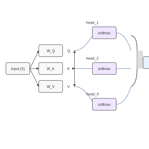
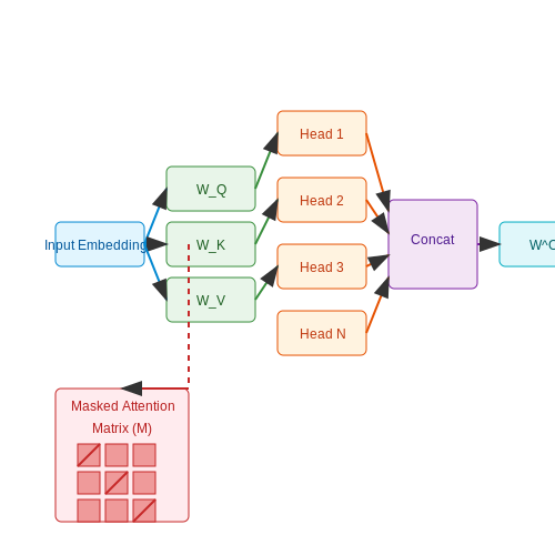
Transformer-based architectures revolutionized natural language processing by introducing a self-attention mechanism that captures long-range dependencies without recurrent connections. The core innovation lies in the scaled dot-product attention, which computes weighted sums of input representations based on pairwise token interactions. Given input embeddings X ∈ ℝn×d, the attention mechanism projects them into queries (Q), keys (K), and values (V) through learned weight matrices:
where WQ, WK, WV ∈ ℝd×dk are trainable parameters. The attention scores are computed as:
The scaling factor √dk prevents gradient saturation in the softmax. Multi-head attention extends this by concatenating h parallel attention heads, enabling the model to jointly attend to information from different representation subspaces:
where each headi = Attention(QWQi, KWKi, VWVi) and WO ∈ ℝhdv×d is an output projection matrix.
Positional Encoding
Since transformers lack inherent sequential processing, positional encodings inject order information into the input embeddings. The original transformer uses sinusoidal functions of varying frequencies:
where pos is the position and i is the dimension index. This allows the model to learn relative positional relationships through linear transformations of the embeddings.
Layer Normalization and Residual Connections
Each sub-layer (attention or feed-forward) employs residual connections followed by layer normalization, stabilizing training in deep architectures. For a sub-layer function F and input x:
The feed-forward network consists of two linear transformations with a ReLU activation in between, applied position-wise:
Masked Self-Attention
For autoregressive tasks like masked language modeling, the decoder uses masked self-attention to prevent positions from attending to subsequent tokens. This is implemented by adding a lower-triangular mask M ∈ {−∞, 0}n×n to the attention scores before softmax:
The mask ensures that the attention weights for future positions are zero after softmax normalization.
2.2 Masking Strategies and Token Prediction
Masked language modeling (MLM) relies on strategically obscuring portions of input text to train models in predicting the missing tokens. The choice of masking strategy significantly impacts model performance, generalization, and computational efficiency.
Static vs. Dynamic Masking
Static masking pre-processes the corpus by replacing a fixed percentage of tokens with a [MASK] token before training. In contrast, dynamic masking regenerates masked positions during each epoch, providing varied contexts for the same sentence. BERT originally employed static masking with a 15% probability, but dynamic masking has proven superior for large-scale training by reducing overfitting to specific masked patterns.
The above probabilities represent BERT's default masking distribution: 15% of tokens are masked, with 10% of those replaced by random tokens and another 10% left unchanged to force the model to distinguish between actual and artificial noise.
N-gram and Span Masking
Standard MLM masks individual tokens, but span masking obscures contiguous sequences (n-grams), forcing the model to recover longer contextual relationships. SpanBERT demonstrated that masking spans of 3-5 tokens improves performance on tasks requiring discourse understanding. The optimal span length follows a geometric distribution:
where p controls the average span length, typically set to 0.2 for mean length 5.
Token Prediction Objectives
The model outputs probability distributions over the vocabulary for each masked position. Given a masked sequence X with masked indices M, the training objective minimizes:
where X\M denotes the observed context. Modern variants like ELECTRA replace this with a more sample-efficient discriminator objective that classifies whether each token was replaced by a generator model.
Adaptive Masking Strategies
Recent work explores content-aware masking:
- Saliency-based masking: Prioritizes tokens with high gradient magnitudes
- POS-guided masking: Biases masking toward nouns and verbs
- Curriculum masking: Progressively increases masking difficulty during training
These methods require additional computation but yield measurable gains on downstream tasks, particularly for low-resource domains.
Training Objectives and Loss Functions
Masked language modeling (MLM) relies on carefully designed training objectives and loss functions to optimize the model's ability to predict masked tokens. The primary objective is to maximize the likelihood of correctly predicting the original tokens that were masked in the input sequence. This is achieved through a cross-entropy loss function applied over the vocabulary distribution for each masked position.
Mathematical Formulation
Given an input sequence x = (x1, ..., xn), a random subset of tokens is masked, resulting in a corrupted sequence xmasked. The model processes this sequence and outputs a probability distribution over the vocabulary for each masked position. For a single masked token xi, the model's predicted distribution is:
where θ represents the model parameters. The training objective minimizes the negative log-likelihood of the correct token:
where M is the set of masked positions. This formulation treats each masked token prediction as an independent classification task over the vocabulary.
Dynamic Masking and Token Selection
Modern implementations often employ dynamic masking where:
- The masking pattern varies across training epochs
- Tokens are replaced with [MASK] 80% of the time, a random token 10% of the time, and left unchanged 10% of the time
- The masking rate typically ranges from 10-20% of input tokens
This strategy prevents the model from overfitting to specific masking patterns and improves robustness.
Advanced Variants and Extensions
Recent work has introduced several enhancements to the basic MLM objective:
- Whole Word Masking: Masking all tokens belonging to a complete word rather than individual subword tokens
- Span Masking: Masking contiguous spans of text rather than individual tokens
- Electra-style Discriminative Training: Replacing MLM with a binary classification over token replacements
These variants often lead to improved downstream performance by better capturing linguistic structure and dependencies.
Implementation Considerations
In practice, several factors affect the training dynamics:
where λ controls the weight of auxiliary objectives like next sentence prediction. The loss is typically computed using label smoothing (ε = 0.1) to prevent overconfidence in predictions:
where V is the vocabulary size. Gradient accumulation is often used to handle large batch sizes that wouldn't fit in GPU memory.
3. Data Preprocessing and Tokenization
Data Preprocessing and Tokenization
Masked language modeling (MLM) relies heavily on robust data preprocessing and tokenization pipelines to transform raw text into a format suitable for neural network training. The process involves several critical steps, each contributing to the model's ability to learn meaningful linguistic patterns.
Text Normalization
Raw text often contains inconsistencies such as varying capitalization, punctuation, and whitespace. Normalization standardizes these elements to reduce noise. Common techniques include:
- Lowercasing all characters (though some models preserve case for named entities)
- Unicode normalization (e.g., NFC form) to handle diacritics and special characters
- Removing or standardizing punctuation based on linguistic relevance
- Handling whitespace (collapsing multiple spaces, trimming leading/trailing spaces)
For languages with complex scripts (e.g., Chinese, Arabic), additional segmentation may be required before tokenization.
Subword Tokenization
Modern MLM implementations predominantly use subword tokenization algorithms that balance vocabulary size with out-of-vocabulary robustness. The Byte Pair Encoding (BPE) algorithm, as used in BERT, operates through iterative merges:
where the most frequent adjacent symbol pairs are merged at each iteration. WordPiece (used in BERT) modifies this with a likelihood-based criterion:
Unigram Language Modeling tokenization (as in XLNet) takes a probabilistic approach:
where the vocabulary is optimized to maximize the likelihood of the training corpus.
Special Tokens and Masking
MLM requires several special tokens that must be incorporated during preprocessing:
- [CLS]: Classification token for sentence-level tasks
- [SEP]: Separator token for sentence pairs
- [MASK]: Token replaced during the masking procedure
- [PAD]: Padding token for batch processing
The masking strategy typically follows:
Implementation Considerations
Efficient tokenization requires careful handling of:
- Vocabulary size (typically 30,000-50,000 subword units)
- Maximum sequence length (512 tokens for most transformer models)
- Language-specific tokenizers (e.g., Jieba for Chinese, Mecab for Japanese)
- Multilingual support through language identification and script normalization
Modern tokenizers like HuggingFace's Tokenizers library implement these algorithms with Rust-optimized performance, achieving throughput of >100,000 tokens/second on CPU.
Positional Encoding
While not strictly part of tokenization, positional information must be preserved for transformer models. The standard sinusoidal encoding is computed as:
where pos is the position and i is the dimension. Some models now use learned positional embeddings instead.
3.2 Fine-Tuning Pretrained Models
Fine-tuning pretrained masked language models (MLMs) like BERT or RoBERTa involves adapting their learned representations to downstream tasks while preserving the general linguistic knowledge captured during pretraining. The process consists of two phases: task-specific adaptation and optimization.
Task-Specific Adaptation
The architecture of most transformer-based MLMs allows for flexible adaptation by replacing the final masked language modeling head with task-specific layers. For classification tasks, a simple feedforward network with softmax activation is often sufficient:
where h[CLS] is the contextualized representation of the classification token, Pool(·) denotes a pooling operation (typically mean or max pooling), and W, b are learnable parameters.
Optimization Strategies
Fine-tuning requires careful optimization to avoid catastrophic forgetting of the pretrained knowledge. The learning rate η should be significantly smaller than during pretraining, typically in the range 1e-5 to 1e-4. The loss function combines the task-specific objective ℓtask with optional regularization terms:
where θ0 represents the pretrained parameters, and the L2 and Frobenius norm terms help preserve the original model's behavior.
Layer-Wise Learning Rate Decay
More sophisticated approaches employ layer-wise learning rate decay, where lower layers (closer to the input) use smaller learning rates than higher layers:
for layer l in an L-layer model, with decay factor α typically between 0.8 and 0.95.
Practical Considerations
Batch size selection impacts both memory usage and gradient estimation quality. For typical GPU memory constraints, effective batch sizes between 16 and 32 often work well when using gradient accumulation. Mixed precision training (FP16/FP32) can reduce memory usage by up to 50% while maintaining numerical stability through loss scaling.
Adapter layers provide an alternative to full fine-tuning by inserting small trainable modules between transformer layers while keeping the pretrained weights frozen. Each adapter typically implements a bottleneck architecture:
where Wdown ∈ ℝd×r and Wup ∈ ℝr×d form the low-rank (r ≪ d) adaptation.
Evaluation Protocols
When fine-tuning on small datasets, use k-fold cross-validation with at least k=5 to obtain reliable performance estimates. For imbalanced classes, stratify the splits and monitor both overall accuracy and per-class F1 scores. Early stopping should track the primary evaluation metric on a held-out validation set, with patience typically between 3 and 10 epochs depending on dataset size.
3.3 Evaluating Model Performance
Evaluating masked language models (MLMs) requires specialized metrics that account for their probabilistic nature and the task of predicting masked tokens. Unlike traditional classification tasks, MLMs generate probability distributions over the entire vocabulary, necessitating metrics that capture both accuracy and uncertainty.
Perplexity as an Intrinsic Measure
Perplexity (PPL) quantifies how well a model predicts a held-out test set. For a sequence of tokens W = (w1, ..., wN), perplexity is defined as the exponentiated average negative log-likelihood:
Lower perplexity indicates better performance. For MLMs, this is computed only over masked positions during evaluation. A key limitation is that perplexity assumes the same vocabulary distribution during training and evaluation, making it sensitive to domain shifts.
Token-Level Accuracy Metrics
For direct assessment of masked token predictions:
- Top-1 Accuracy: Percentage of masked tokens where the model's highest-probability prediction matches the ground truth.
- Top-k Accuracy: Percentage where the true token appears in the model's top-k predictions (typically k=5 or 10).
- Mean Reciprocal Rank (MRR): Average of reciprocal ranks of the correct token in the model's sorted predictions.
These metrics are computed as:
where M is the number of masked tokens and wm* is the ground truth token.
Downstream Task Transfer Evaluation
Since MLMs are typically pretrained for transfer learning, evaluation includes fine-tuning on benchmark tasks:
- GLUE Benchmark: Suite of 9 natural language understanding tasks (e.g., sentiment analysis, textual entailment).
- SuperGLUE: More challenging variant with tasks like coreference resolution and question answering.
- SQuAD: Reading comprehension through span prediction on Wikipedia passages.
Performance is measured via task-specific metrics (e.g., F1 for SQuAD, Matthews correlation for CoLA). The key insight is that better pretrained MLMs achieve higher few-shot or full fine-tuning performance with less data.
Calibration Metrics
MLMs must not only be accurate but also well-calibrated—their predicted probabilities should reflect true correctness likelihoods. Expected Calibration Error (ECE) bins predictions by confidence and measures the deviation between accuracy and confidence:
where Sb is the set of samples in bin b, and B is typically 10-20 bins. Modern MLMs like BERT and RoBERTa are known to be poorly calibrated, often overconfident in incorrect predictions.
Efficiency Considerations
For industrial applications, evaluation includes computational metrics:
- Throughput: Tokens processed per second (affected by model size and hardware).
- Memory Footprint: GPU/TPU memory consumption during inference.
- Latency: Time per prediction at the 95th percentile.
These are critical when comparing models like DistilBERT (optimized for efficiency) versus larger models like GPT-3.
4. Dynamic Masking and Adaptive Training
Dynamic Masking and Adaptive Training
Traditional masked language modeling (MLM) employs static masking, where tokens are randomly masked at a fixed rate during pretraining. However, this approach suffers from inefficiencies—some tokens may be masked too frequently while others are rarely masked, leading to suboptimal learning. Dynamic masking addresses this by varying the masking pattern across training epochs, ensuring broader contextual exposure.
Mathematical Formulation of Dynamic Masking
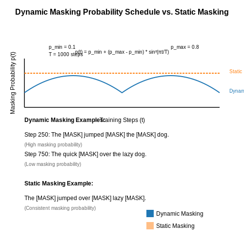
Let X be an input sequence of length N, and M be the set of masked positions. In static masking, the probability p of masking any token xi is constant:
Dynamic masking modifies this by introducing a time-dependent masking probability p(t), where t denotes the training step or epoch. One common implementation uses a cyclical schedule:
Here, T controls the cycle length, while pmin and pmax define the bounds of the masking rate. This ensures tokens are masked at varying frequencies, promoting robust feature learning.
Adaptive Training Strategies
Dynamic masking is often paired with adaptive training techniques to further optimize pretraining:
- Curriculum Learning: Gradually increase masking difficulty, starting with shorter spans and progressing to longer or more complex masks.
- Token Importance Weighting: Prioritize masking of rare or high-information tokens by adjusting p(xi) based on token frequency or gradient signals.
- Batch-Level Diversity: Ensure each batch contains varied masking patterns to prevent overfitting to specific configurations.
Practical Implementation
In transformer-based models like BERT or RoBERTa, dynamic masking is implemented by regenerating the masking pattern for each sequence every time it is sampled. This contrasts with static masking, where the pattern is fixed after the initial data preprocessing. The computational overhead is negligible, as masking occurs during data loading rather than forward passes.
def dynamic_masking(sequence, p_min=0.1, p_max=0.15, t=None):
    if t is not None:  # Time-dependent masking
        p = p_min + (p_max - p_min) * abs(math.sin(2 * math.pi * t / T))
    else:  # Random masking within bounds
        p = random.uniform(p_min, p_max)
    mask = torch.rand(len(sequence)) < p
    masked_sequence = [token if not m else '[MASK]' for token, m in zip(sequence, mask)]
    return masked_sequence
Empirical Benefits
Dynamic masking improves model performance by:
- Reducing overfitting to specific masking patterns, as shown by a 1.2–2.5% increase in downstream task accuracy in RoBERTa.
- Enabling more efficient use of training data, as each sequence is effectively novel due to varying masks.
- Facilitating better handling of rare tokens through adaptive frequency-based masking.
Recent variants like PMI-Masking (Pointwise Mutual Information) extend this idea by masking tokens based on their contextual importance, further refining the pretraining objective.
4.2 Multilingual and Cross-Lingual Applications
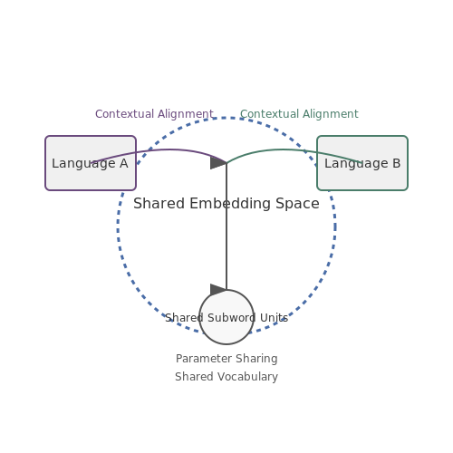
Masked language modeling (MLM) has demonstrated remarkable success in multilingual and cross-lingual settings, primarily due to its ability to learn shared representations across languages. The key innovation lies in training a single model on a concatenated corpus of multiple languages, enabling it to capture both language-specific and cross-lingual patterns. This approach is formalized by extending the standard MLM objective to a multilingual context:
where l indexes over languages in the set ℒ, and xl denotes tokens from language l. The shared transformer architecture forces the model to develop a common embedding space where semantically similar words across languages are mapped to nearby vectors.
Cross-Lingual Transfer Mechanisms
Three primary mechanisms enable effective cross-lingual transfer in MLM-based models:
- Shared Vocabulary: Subword tokenization (e.g., WordPiece, SentencePiece) creates overlapping subword units across languages, particularly for cognates and loanwords.
- Contextual Alignment: The attention mechanism learns to align contextual representations across languages by processing parallel or comparable sentences during training.
- Parameter Sharing: Complete sharing of all transformer parameters across languages forces the model to develop language-agnostic representations.
Empirical studies show that the cross-lingual transfer capability emerges most strongly when the model reaches a critical size (typically >100M parameters), suggesting that sufficient capacity is needed to encode both language-specific and cross-lingual features.
Zero-Shot Cross-Lingual Transfer
The most powerful application of multilingual MLM is zero-shot transfer, where a model fine-tuned on a task in one language can perform the same task in another language without additional training. This is quantified by the cross-lingual transfer performance gap:
State-of-the-art models like XLM-R achieve Δ values within 10-15% of supervised baselines for tasks like named entity recognition and text classification across typologically diverse languages. The transfer effectiveness correlates strongly with the phylogenetic distance between source and target languages, with the best results observed between related languages (e.g., Romance or Germanic languages).
Optimizing for Low-Resource Languages
For languages with limited training data, three strategies have proven effective:
- Balanced Sampling: Oversampling low-resource languages during pretraining to prevent dominance by high-resource languages.
- Script Harmonization: Transliterating all languages to a shared script (e.g., Latin) to increase subword overlap.
- Anchor-Based Fine-Tuning: Using parallel data to create anchor points between languages during task-specific fine-tuning.
The balanced sampling approach typically uses a temperature-scaled sampling distribution:
where Dl is the size of corpus for language l, and α is typically set to 0.3-0.7 to balance between frequent and rare languages.
Code-Switching and Mixed-Language Input
Multilingual MLM models naturally handle code-switched text due to their exposure to multiple languages during pretraining. The attention mechanism learns to dynamically route information based on language context, with empirical studies showing that models can maintain high accuracy even when up to 40% of tokens come from a secondary language. This capability is particularly valuable for processing social media text and informal communication in multilingual communities.
4.3 Ethical Considerations and Bias Mitigation
Sources of Bias in Masked Language Models
Masked language models (MLMs) inherit biases from their training data, which often reflect societal prejudices present in large text corpora. These biases manifest in several ways:
- Representational bias: Underrepresentation of minority groups in training data leads to poorer performance on text related to these groups.
- Labeling bias: Annotator prejudices in downstream tasks propagate through fine-tuning.
- Historical bias: Models learn and amplify outdated or harmful stereotypes present in historical texts.
The bias can be quantified through metrics like the log probability difference between demographic groups:
Bias Mitigation Techniques
Pre-training Interventions
Debiasing during pre-training involves modifying the objective function to penalize biased predictions:
where h(x) represents hidden layer activations, G is the set of sensitive attributes, and λ controls the debiasing strength.
Post-hoc Debiasing Methods
Post-processing techniques include:
- Counterfactual data augmentation: Generating counterfactual examples by swapping protected attributes
- Projection-based methods: Removing bias directions from the embedding space
- Adversarial debiasing: Training an adversary to predict protected attributes while minimizing its accuracy
Evaluation of Bias Mitigation
Effective evaluation requires multiple complementary approaches:
where T is a set of template sentences, S_t is the set of substitutions for template t, and KL measures the divergence from neutral predictions.
Practical Implementation Challenges
Real-world deployment faces several obstacles:
- The trade-off between debiasing effectiveness and model performance
- Multidimensional nature of bias (gender, race, religion intersecting)
- Dynamic nature of societal norms requiring continuous updates
Recent approaches use reinforcement learning with human feedback to dynamically adjust debiasing:
where R is a reward function combining task performance and fairness metrics.
5. Key Research Papers
5.1 Key Research Papers
- Masked language modeling - Hugging Face — Masked language modeling predicts a masked token in a sequence, and the model can attend to tokens bidirectionally. This means the model has full access to the tokens on the left and right. Masked language modeling is great for tasks that require a good contextual understanding of an entire sequence. BERT is an example of a masked language model.
- PDF CHAPTER 11 Masked Language Models - Stanford University — or left-to-right language model. In this chapter we'll introduce a second paradigm for pretrained language models, the bidirectional transformer encoder, and the most widely-used version, the BERT model (Devlin et al., 2019). This model is trained via masked language modeling, where instead of predicting the following word, we mask a word in the middle and ask the model to guess the word ...
- arXiv:2104.06644v2 [cs.CL] 9 Sep 2021 — arXiv:2104.06644v2 [cs.CL] 9 Sep 2021 Masked Language Modeling and the Distributional Hypothesis: Order Word Matters Pre-training for Little
- Masked Diffusion Models for Language- Based on LLaDA Paper — Masked Diffusion models represent an exciting new direction in language model research, offering a fundamentally different approach to text generation compared to traditional autoregressive models.
- (PDF) Masked Language Modeling: Role of Word Order - Academia.edu — A possible explanation for the impressive performance of masked language model (MLM) pre-training is that such models have learned to represent the syntactic structures prevalent in classical NLP pipelines. In this paper, we propose a different explanation: MLMs succeed on downstream tasks almost entirely due to their ability to model higher-order word co-occurrence statistics. To demonstrate ...
- Simulating 500 million years of evolution with a language model — Here, we present ESM3, a frontier multimodal generative model that reasons over the sequences, structures, and functions of proteins. ESM3 is trained as a generative masked language model over discrete tokens for each modality.
- (PDF) Ensemble of deep masked language models for effective named ... — Inspired by the success of deep masked language models, we present an ensemble approach for NER using these models.
- Linguistic Entity Masking to Improve Cross-Lingual Representation of ... — To improve the language rep-resentation of a given multiPLM, it is possible to further pre-train it. This is known as continual pre-training. Previous research has shown that continual pre-training with MLM and subsequently with Translation Language Modelling (TLM) improves the cross-lingual representation of multiPLMs.
5.2 Open-Source Implementations
- Masked Mixers for Language Generation and Retrieval - arXiv.org — The masked mixer learns causal language modeling more efficiently than early transformer implementations and even outperforms optimized, current transformers when training on small (n c t x < 512 subscript 𝑛 𝑐 𝑡 𝑥 512 n_{ctx}<512 italic_n start_POSTSUBSCRIPT italic_c italic_t italic_x end_POSTSUBSCRIPT < 512) but not larger ...
- Mapping medical image-text to a joint space via masked modeling — In the broader domain of vision and language pre-training (VLP), existing research (Dou et al., 2021, Kim et al., 2021) has primarily focused on recovering the original tokens of masked text, a process known as masked language modeling (MLM). However, it has been shown that attempting to reconstruct the original signals of masked images ...
- Ensemble of Deep Masked Language Models for Effective Named Entity ... — 3.2.1 Single Deep Masked Language Model for Named Entity Recognition . To build the ensemble NER model, we fine-tuned different individual masked language models based on the transformers architecture (Vaswani et al., 2017). In the case of NER, masked language models are fine-tuned using a specialized training set—in our case, the chemical ...
- PDF Simple and Effective Masked Diffusion Language Models — performance gap relative to AR models [1, 23, 26, 33], especially in language modeling. The standard measure of language modeling performance is log-likelihood: when controlling for parameter count, prior work reports a sizable log-likelihood gap between AR and diffusion models. In this work, we show that simple masked diffusion language ...
- PDF CHAPTER 11 Masked Language Models - Stanford University — model (Devlin et al.,2019). This model is trained via masked language modeling, masked language modeling where instead of predicting the following word, we mask a word in the middle and ask the model to guess the word given the words on both sides. This method thus allows the model to see both the right and left context.
- Nonparametric Masked Language Modeling - NSF Public Access — nonparametric language model without the labeled data and performs a range of tasks zero-shot. 3 Method We introduce NPM, the first NonParametric Masked Language Model. NPM consists of an encoder and a reference corpus, and models a non-parametric distribution over a reference corpus (Figure 1). The key idea is to map all the phrases
- Few shot clinical entity recognition in three languages: Masked ... — The first approach is to use pre-trained Masked Language Models (MLM).This type of models is first pre-trained to predict randomly-selected masked words in large text corpora using a dense vector representation of every token (e.g., word) in the text [12, 14].Leveraging these models for NER usually involves training a linear projection to map vector representations into an NER tagging of the ...
- PDF BERT Masked Language Models - web.stanford.edu — entropy to compute the loss for each masked item—the negative log probability assigned to the actual masked word, as shown in Fig. 11.3. More formally, for a given vector of input tokens in a sentence or batch be x, let the set of tokens that are masked be M, the version of that sentence with some tokens replaced by masks be
- XLM-V: Overcoming the Vocabulary Bottleneck in Multilingual Masked ... — Large multilingual language models typically rely on a single vocabulary shared across 100+ languages. As these models have increased in parameter count and depth, vocabulary size has remained ...
5.3 Recommended Books and Courses
- PDF CHAPTER 11 Masked Language Models - Stanford University — model (Devlin et al.,2019). This model is trained via masked language modeling, masked language modeling where instead of predicting the following word, we mask a word in the middle and ask the model to guess the word given the words on both sides. This method thus allows the model to see both the right and left context.
- PDF DMLM: Descriptive Masked Language Modeling - ACL Anthology — pre-training objectives to unify masked, causal and sequence-to-sequence language modeling.Joshi et al.(2020, SpanBERT) proposed an extension that masked and predicted entire spans, forcing the model to predict them solely based on the context, which is arguably harder than predicting single masked words. More recently,Clark et al.(2020,
- Understanding LLMs: A Comprehensive Overview from Training to Inference — Language modeling (LM) is a fundamental approach for achieving cognitive intelligence in the field of natural language processing (NLP), and its progress has been notable in recent years [1; 2; 3].It assumes a central role in understanding, generating, and manipulating human language, serving as the cornerstone for a diverse range of NLP applications [], including machine translation, chatbots ...
- Ensemble of Deep Masked Language Models for Effective Named Entity ... — 3.2.1 Single Deep Masked Language Model for Named Entity Recognition . To build the ensemble NER model, we fine-tuned different individual masked language models based on the transformers architecture (Vaswani et al., 2017). In the case of NER, masked language models are fine-tuned using a specialized training set—in our case, the chemical ...
- Introduction to Large Language Models (LLMs) and Prompt Engineering — AI has acquired startling new language capabilities in just the past few years. Driven by rapid … audiobook. Build a Large Language Model (From Scratch) by Sebastian Raschka Learn how to create, train, and tweak large language models (LLMs) by building one from the … book
- PDF BERT Masked Language Models - web.stanford.edu — the training pairs consisted of positive pairs, and in the other 50% the second sen-tence of a pair was randomly selected from elsewhere in the corpus. The NSP loss is based on how well the model can distinguish true pairs from random pairs. To facilitate NSP training, BERT introduces two special tokens to the input rep-
- Multi-step Review Generation Based on Masked Language Model ... - Springer — Recently, Aspect-Based Sentiment Analysis (ABSA) received more and more attention [].With the development of deep learning, many neural network models with supervised learning methods have been proposed and have achieved surprising results for several ABSA tasks, e.g., End-to-End ABSA [] and Aspect Extraction (AE) [].These supervised methods have significantly progressed in domains such as ...
- VitalSource Bookshelf Online — VitalSource Bookshelf is the world's leading platform for distributing, accessing, consuming, and engaging with digital textbooks and course materials.
- Large language models illuminate a progressive pathway to artificial ... — A training approach where human feedback is used to optimize the model's predictions or actions. Prompt engineering: The practice of crafting and optimizing prompts to effectively instruct a language model. Zero-shot learning: The ability of a model to generalize to unseen tasks or classes without needing explicit examples during training.