Neural Topic Modeling with BERTopic
1. What is Topic Modeling?
What is Topic Modeling?
Topic modeling is an unsupervised machine learning technique for discovering latent semantic structures in large text corpora. It operates by statistically analyzing word co-occurrence patterns to group documents into clusters, or topics, where each topic is represented as a probability distribution over words. Formally, given a corpus of N documents and a vocabulary of size V, topic modeling aims to infer:
where w denotes a word, d a document, and z a latent topic. The model learns two distributions: P(w|z) (words per topic) and P(z|d) (topics per document).
Historical Context and Evolution
Early approaches like Latent Semantic Indexing (LSI) used singular value decomposition to project documents into a lower-dimensional space. Probabilistic Latent Semantic Analysis (pLSA) introduced a generative framework but suffered from overfitting. Latent Dirichlet Allocation (LDA), proposed by Blei et al. in 2003, became the dominant method by introducing Dirichlet priors to model document-topic and topic-word distributions, enabling better generalization.
Neural Advancements
Traditional methods rely on bag-of-words representations, discarding word order and contextual semantics. Neural topic models, such as those leveraging BERT embeddings, address this by:
- Using dense vector representations from transformer architectures to capture contextual word meanings.
- Clustering document embeddings in a continuous semantic space rather than discrete word counts.
- Enabling dynamic topic modeling where topics evolve over time.
Applications
Topic modeling is widely used in:
- Document organization: Automatically tagging research papers or legal documents.
- Trend analysis: Identifying shifts in public opinion from social media.
- Recommendation systems: Enhancing content discovery by linking related articles.
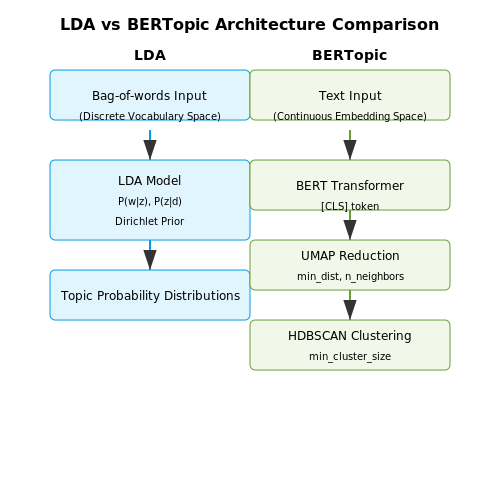
For example, BERTopic combines BERT embeddings with dimensionality reduction (UMAP) and clustering (HDBSCAN) to produce interpretable topics while preserving semantic nuances lost in count-based models.
Traditional vs. Neural Topic Modeling
Probabilistic Foundations of Traditional Topic Models
Traditional topic modeling approaches like Latent Dirichlet Allocation (LDA) operate on bag-of-words representations using discrete probability distributions. The core generative process assumes:
where w represents words, d documents, and z latent topics. This formulation suffers from the curse of dimensionality in vocabulary space and cannot capture semantic relationships between words. The Dirichlet prior:
imposes strong assumptions about topic distributions that may not hold for real-world text data.
Neural Paradigm Shift in Topic Modeling
Neural topic models replace discrete distributions with continuous embeddings from deep neural networks. BERTopic leverages transformer architectures to produce dense document representations:
where the [CLS] token embedding captures document-level semantics. This enables:
- Non-linear relationships between words and topics
- Context-aware representations (polysemy handling)
- Cross-lingual topic modeling capabilities
Dimensionality Reduction Tradeoffs
Traditional LDA operates directly in vocabulary space (typically 104-105 dimensions), while neural approaches first project documents into lower-dimensional spaces (typically 128-768 dimensions). BERTopic employs UMAP for non-linear dimensionality reduction:
This preserves both local and global structure better than linear methods like PCA or LSA used in traditional pipelines.
Clustering Algorithm Evolution
Where LDA uses collapsed Gibbs sampling for inference:
BERTopic employs density-based clustering (HDBSCAN) on the reduced embeddings:
This eliminates the need to pre-specify topic numbers and handles outliers more effectively.
Representational Power Comparison
Traditional models capture word co-occurrence statistics, while neural models learn hierarchical semantic features. The table below contrasts key characteristics:
| Feature | Traditional (LDA) | Neural (BERTopic) |
|---|---|---|
| Representation Space | Discrete (Vocabulary) | Continuous (Embedding) |
| Context Handling | Bag-of-words | Full sequence context |
| Dimensionality | O(V) | O(d), d ≪ V |
| Training Objective | Likelihood maximization | Representation learning |
Practical Considerations
Neural approaches require GPU acceleration for transformer inference, while traditional models can run on CPUs. However, BERTopic's two-phase design (embedding then clustering) enables:
- Incremental topic modeling via cached embeddings
- Fine-grained control over clustering parameters
- Integration of domain-specific language models
Why BERTopic?
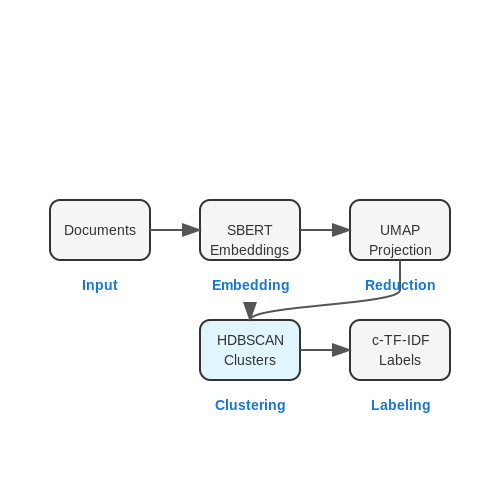
Traditional topic modeling techniques like Latent Dirichlet Allocation (LDA) and Non-Negative Matrix Factorization (NMF) rely on bag-of-words representations, which discard semantic relationships between words. While these methods are computationally efficient, they struggle with polysemy, synonymy, and contextual meaning—critical aspects of natural language understanding. BERTopic addresses these limitations by leveraging transformer-based embeddings, specifically sentence-BERT (SBERT), to capture dense, context-aware representations of text.
Semantic Richness Through Embeddings
BERTopic's core strength lies in its use of pre-trained language models to generate document embeddings. Unlike LDA, which operates on term-frequency matrices, BERTopic first maps documents to a high-dimensional semantic space using SBERT. The resulting embeddings preserve syntactic and semantic relationships, enabling the model to cluster documents based on meaning rather than lexical overlap. Mathematically, given a document d, its embedding e is computed as:
where the dimensionality depends on the underlying transformer model (e.g., 768 for all-MiniLM-L6-v2). This approach captures fine-grained semantic distinctions, such as differentiating "bank" as a financial institution versus a riverbank.
Dimensionality Reduction and Clustering
After embedding, BERTopic reduces dimensionality using UMAP (Uniform Manifold Approximation and Projection), which preserves local and global structures better than linear methods like PCA. The reduced embeddings are then clustered using HDBSCAN, a density-based algorithm that automatically detects the number of topics and handles outliers. The combined pipeline optimizes:
where C is the set of cluster centroids. HDBSCAN's soft clustering further allows documents to remain unassigned if they lack topical relevance, reducing noise in the final output.
Dynamic Topic Representation
BERTopic generates interpretable topic labels by applying class-based TF-IDF (c-TF-IDF) to clustered documents. This technique reweights terms based on their importance within a topic relative to the entire corpus, avoiding the need for manual label curation. For a term w in topic k, its score is:
where fw,k is the frequency of w in topic k, N is the total number of topics, and nw is the number of topics containing w. This results in discriminative labels that reflect each topic's unique vocabulary.
Practical Advantages
- Multilingual Support: SBERT embeddings enable cross-lingual topic modeling without parallel corpora.
- Handling Short Texts: Embeddings outperform LDA on tweets or product reviews by capturing context beyond word co-occurrence.
- Online Learning: Incremental UMAP and HDBSCAN allow topic updates with streaming data, unlike batch-only LDA.
2. Embedding Generation with BERT
Embedding Generation with BERT
BERT (Bidirectional Encoder Representations from Transformers) generates contextualized word embeddings by leveraging transformer architecture. Unlike traditional word embeddings (e.g., Word2Vec, GloVe), BERT captures bidirectional context, making it highly effective for semantic representation in topic modeling. The embedding process involves tokenization, positional encoding, and multi-head attention mechanisms.
Tokenization and Input Representation
BERT uses WordPiece tokenization to split text into subword units, addressing out-of-vocabulary issues. Each input sequence is prepended with a [CLS] token and separated by a [SEP] token for sentence pairs. The input embedding E is the sum of:
- Token embeddings (subword representations)
- Position embeddings (sequential order information)
- Segment embeddings (distinguishing between sentences in paired inputs)
Transformer Encoder Layers
BERT's transformer encoder stacks multiple identical layers, each containing:
- Multi-head self-attention: Computes attention scores between all tokens in parallel, enabling context-aware representations.
- Feed-forward networks: Applies non-linear transformations to attention outputs.
- Layer normalization and residual connections: Stabilizes training and mitigates vanishing gradients.
The self-attention mechanism for a single head is defined as:
where Q, K, and V are learned query, key, and value matrices, and dk is the dimension of the key vectors.
Pooling Strategies for Document Embeddings
To derive a fixed-length document embedding from BERT's token-level outputs, common approaches include:
- [CLS] token pooling: Uses the embedding of the first token, fine-tuned for classification tasks.
- Mean/max pooling: Aggregates token embeddings via averaging or max operation.
- Weighted pooling: Applies attention-based weighting to emphasize salient tokens.
For BERTopic, mean pooling is often preferred for its balance between computational efficiency and semantic retention:
where N is the number of tokens, and hi is the hidden state of the i-th token.
Dimensionality Reduction
BERT embeddings are high-dimensional (e.g., 768 for BERT-base), necessitating reduction for clustering. UMAP (Uniform Manifold Approximation and Projection) is commonly used due to its ability to preserve local and global structures:
where ncomponents is typically set between 2 and 5 for topic modeling.
Practical Considerations
- Batch processing: Leverage GPU parallelism by processing documents in batches.
- Model variants: Pre-trained models like all-MiniLM-L6-v2 offer a trade-off between speed and accuracy.
- Fine-tuning: Domain-specific corpora can improve embedding quality via further pretraining.
Dimensionality Reduction with UMAP
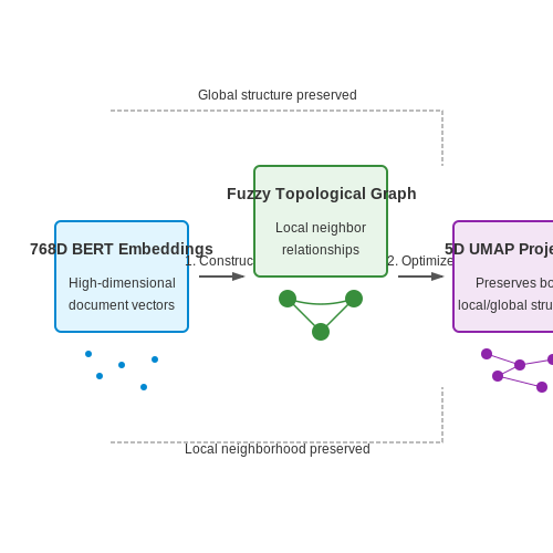
BERTopic leverages Uniform Manifold Approximation and Projection (UMAP) for dimensionality reduction of high-dimensional document embeddings before clustering. UMAP is preferred over traditional methods like PCA due to its ability to preserve both local and global structure in the data, making it particularly effective for topic modeling where semantic relationships between documents are crucial.
UMAP Theoretical Foundations
UMAP operates on the principle of constructing a high-dimensional weighted graph representation of the data and optimizing a low-dimensional layout to preserve the graph's topological structure. The mathematical foundation consists of three key components:
- Fuzzy topological representation: For each point xi, a neighborhood is defined using an adaptive exponential kernel:
- Graph construction: The high-dimensional probabilities are symmetrized to create a fuzzy simplicial set:
- Low-dimensional optimization: The cross-entropy between the high and low-dimensional representations is minimized using stochastic gradient descent.
Practical Implementation in BERTopic
In BERTopic, UMAP serves two critical functions:
- Reduces typically 768-dimensional BERT embeddings to a more manageable size (default 5 dimensions)
- Preserves semantic relationships between documents while removing noise
The key parameters that significantly impact topic quality are:
- n_neighbors: Controls local vs. global structure balance (default 15)
- n_components: Output dimensionality (default 5)
- min_dist: Minimum distance between points in low-dimensional space (default 0.0)
- metric: Distance metric (default 'cosine' for text embeddings)
from bertopic import BERTopic
from umap import UMAP

umap_model = UMAP(n_neighbors=15,
                 n_components=5,
                 min_dist=0.0,
                 metric='cosine',
                 random_state=42)

topic_model = BERTopic(umap_model=umap_model)
Advanced Optimization Techniques
For research-grade implementations, consider these optimizations:
- Dynamic neighborhood sizing: Adjust n_neighbors based on dataset size (logarithmic scaling)
- Ensemble UMAP: Combine multiple UMAP projections to improve stability
- Custom distance metrics: Incorporate domain-specific similarity measures
The choice of UMAP parameters significantly affects HDBSCAN clustering performance downstream. Empirical studies show that n_components between 5-20 works best for most text corpora, with higher values preserving more variance but increasing computational cost.
2.3 Clustering with HDBSCAN
HDBSCAN (Hierarchical Density-Based Spatial Clustering of Applications with Noise) extends DBSCAN by converting it into a hierarchical clustering algorithm and extracting stable clusters through a density-based approach. Unlike traditional centroid-based methods like k-means, HDBSCAN identifies clusters of varying densities while automatically determining the optimal number of clusters.
Core Algorithm
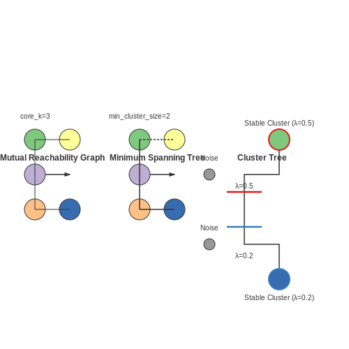
The algorithm operates in four key steps:
- Mutual Reachability Distance Graph: Constructs a weighted graph where edge weights represent the mutual reachability distance, defined as:
where $$\text{core}_k(x)$$ is the distance to the k-th nearest neighbor of point $$x$$.
- Minimum Spanning Tree (MST): Computes the MST of the mutual reachability graph using Prim's or Kruskal's algorithm.
- Hierarchical Cluster Tree: Converts the MST into a hierarchy of connected components by iteratively removing edges in decreasing order of distance.
- Cluster Stability Selection: Extracts flat clusters by optimizing for persistence across density thresholds using the stability metric:
Key Advantages in Topic Modeling
HDBSCAN's non-parametric nature makes it particularly suitable for topic modeling because:
- It automatically handles varying cluster densities in semantic spaces
- Requires no predefined number of topics (unlike LDA or NMF)
- Identifies noise points as outliers rather than forcing them into clusters
- Preserves hierarchical relationships between topics
Practical Implementation
The BERTopic implementation uses HDBSCAN's soft clustering capabilities to:
- Assign documents to topics based on relative cluster membership probabilities
- Handle overlapping topic boundaries through fuzzy clustering
- Adjust cluster granularity via the min_cluster_size parameter
from bertopic import BERTopic
from hdbscan import HDBSCAN

# Custom HDBSCAN configuration
hdbscan_model = HDBSCAN(min_cluster_size=15,
                        metric='euclidean',
                        cluster_selection_method='eom',
                        prediction_data=True)

topic_model = BERTopic(hdbscan_model=hdbscan_model)
Parameter Optimization
Critical parameters for topic modeling applications include:
- min_cluster_size: Controls the minimum topic size (typically 10-50 for document clustering)
- cluster_selection_epsilon: Sets a distance threshold for cluster merging
- min_samples: Determines local density requirements (lower values increase sensitivity)
The optimal parameterization depends on the embedding space dimensionality and document corpus characteristics. A grid search over these parameters combined with topic coherence validation often yields the best results.
Topic Representation and Visualization
BERTopic generates interpretable topic representations by leveraging the semantic embeddings from transformer models. Each topic is characterized by a set of representative terms, which are extracted using a class-based TF-IDF (c-TF-IDF) approach. This method reweights term frequencies within topics relative to their frequencies across the entire corpus, ensuring discriminative and meaningful topic descriptors.
Class-based TF-IDF Formulation
The c-TF-IDF score for term t in topic k is computed as:
where:
- ft,k is the frequency of term t in topic k,
- N is the total number of topics,
- ft is the frequency of term t across all topics.
This formulation emphasizes terms that are frequent within a specific topic but relatively rare in others, enhancing topic distinctiveness.
Visualization Techniques
BERTopic supports multiple visualization methods to facilitate topic interpretation:
1. Intertopic Distance Map
This visualization projects topics into a 2D space using dimensionality reduction techniques like UMAP or PCA, where the distance between topics reflects their semantic similarity. Topics are represented as bubbles, with size proportional to their prevalence in the corpus.
2. Topic Word Scores
A bar chart displays the top n terms per topic with their c-TF-IDF scores, allowing quick assessment of term relevance. The chart is interactive in Jupyter environments, enabling dynamic exploration of topic compositions.
3. Hierarchical Clustering
Topics can be organized into a dendrogram to reveal their hierarchical relationships. This is particularly useful for identifying meta-topics or merging similar topics during post-processing.
Practical Implementation
The visualization tools are accessible through BERTopic's API. For example, generating an intertopic distance map requires:
from bertopic import BERTopic
topic_model = BERTopic()
topics, probs = topic_model.fit_transform(docs)
topic_model.visualize_topics()
Customizations like adjusting the UMAP parameters (n_neighbors, min_dist) or switching to PCA can refine the layout. For hierarchical visualization:
topic_model.visualize_hierarchy()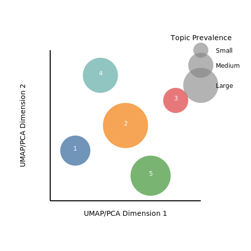
3. Installing and Setting Up BERTopic
Installing and Setting Up BERTopic
BERTopic requires Python 3.7 or higher and leverages several key dependencies including sentence-transformers for embedding generation, UMAP for dimensionality reduction, and HDBSCAN for clustering. The package can be installed via pip:
pip install bertopicGPU Acceleration
For optimal performance with large datasets, enable GPU acceleration by installing PyTorch with CUDA support. The following command installs PyTorch 1.12+ with CUDA 11.3:
pip install torch torchvision torchaudio --extra-index-url https://download.pytorch.org/whl/cu113Custom Embedding Models
BERTopic supports custom sentence transformers from HuggingFace. To use a non-default model, specify it during initialization:
from bertopic import BERTopic
from sentence_transformers import SentenceTransformer

embedding_model = SentenceTransformer("all-mpnet-base-v2")
topic_model = BERTopic(embedding_model=embedding_model)
Dimensionality Reduction Configuration
The default UMAP parameters can be adjusted to optimize topic separation. Key hyperparameters include:
These can be passed as a dictionary to the UMAP model:
umap_params = {
    "n_neighbors": 15,
    "min_dist": 0.0,
    "n_components": 5,
    "metric": "cosine"
}
topic_model = BERTopic(umap_model=umap_params)
Clustering with HDBSCAN
HDBSCAN's density-based clustering requires careful parameter tuning. The minimum cluster size (min_cluster_size) and minimum samples (min_samples) significantly impact results:
hdbscan_params = {
    "min_cluster_size": 10,
    "min_samples": 5,
    "metric": "euclidean",
    "cluster_selection_method": "eom"
}
topic_model = BERTopic(hdbscan_model=hdbscan_params)
Verifying Installation
Confirm successful installation by generating a basic topic model on sample text:
from bertopic import BERTopic
docs = ["Example document one", "Another example document"]
topic_model = BERTopic()
topics, probs = topic_model.fit_transform(docs)
3.2 Preprocessing Text Data
Effective preprocessing is critical for neural topic modeling, as raw text often contains noise that degrades the quality of embeddings and clustering. BERTopic leverages transformer-based embeddings, which are robust to minor variations, but systematic preprocessing ensures optimal performance.
Text Normalization
Text normalization standardizes linguistic variations while preserving semantic meaning. Key steps include:
- Lowercasing: Reduces vocabulary size by treating "Machine" and "machine" as identical tokens. However, this may degrade performance in case-sensitive domains (e.g., named entity recognition).
- Unicode normalization: Converts characters to canonical forms using NFKC (Normalization Form Compatibility Composition), merging visually identical symbols (e.g., "ℍ" → "H").
- Contraction expansion: Replaces "don't" with "do not" to prevent tokenizer artifacts. This requires careful handling to avoid over-normalization (e.g., "LLC" should remain intact).
Noise Removal
Domain-specific noise patterns require targeted removal strategies:
Where \( f_d(t) \) is term frequency in domain corpus, \( f_c(t) \) in common corpora, and \( \text{df}(t) \) is document frequency. Terms with high NoiseScore are candidates for removal.
Specialized Filters
- HTML/XML tags: Removed using regex patterns like
<\/?[a-z][^>]*>with allowance for mathematical content (e.g.,<matrix>in technical papers). - Citation markers: Pattern-based removal of "[1]" or "(Smith et al., 2020)" while preserving in-text references.
- Numerical artifacts: Threshold-based filtering of rare alphanumeric combinations (e.g., "X12-345") while keeping chemically relevant terms (e.g., "H2O").
Tokenization Refinement
BERT's WordPiece tokenizer benefits from preprocessing adjustments:
from transformers import AutoTokenizer
tokenizer = AutoTokenizer.from_pretrained("bert-base-uncased")

# Custom preprocessing pipeline
def preprocess(text):
    text = text.replace("_", " ")  # Preserve subword boundaries
    tokens = tokenizer.tokenize(text)
    return [t for t in tokens if not t.startswith("##")
            and len(t) > 1]  # Filter subword fragments
This approach maintains syntactic coherence while reducing vocabulary sparsity. For technical domains, preserving hyphenated compounds (e.g., "state-of-the-art") through selective whitespace manipulation improves embedding quality.
Stopword Optimization
Traditional stopword lists often remove semantically rich terms in specialized domains. A dynamic approach computes term relevance:
Where TopicCoherence measures the term's association strength with other high-probability terms in candidate topics. Domain-specific stopwords are identified when Relevance(w) < θ (typically θ ≈ 0.1 for scientific texts).
Lemmatization Trade-offs
While lemmatization ("running" → "run") reduces morphological variation, it can:
- Degrade performance for proper nouns ("Windows" → "window")
- Introduce ambiguity in polysemous words ("leaves" → "leaf" or "leave")
An optimized pipeline uses POS-tagging to apply lemmatization only to verbs and adjectives, preserving noun forms. SpaCy's rule-based system provides sufficient accuracy for this filtered approach:
import spacy
nlp = spacy.load("en_core_web_sm", disable=["parser", "ner"])

def selective_lemmatize(text):
    doc = nlp(text)
    return [token.lemma_ if token.pos_ in {"VERB", "ADJ"}
            else token.text for token in doc]
Training the BERTopic Model
BERTopic leverages transformer-based embeddings and clustering techniques to generate interpretable topics. The training process consists of three primary stages: document embedding, dimensionality reduction, and clustering. Each stage is optimized for scalability and semantic coherence.
Document Embedding with Sentence Transformers
BERTopic uses pre-trained language models from the Sentence Transformers library to generate dense vector representations of documents. The default model is all-MiniLM-L6-v2, which balances speed and performance. Given a corpus of documents D = {d₁, d₂, ..., dₙ}, each document dᵢ is mapped to an embedding vector eᵢ ∈ ℝᵈ, where d is the embedding dimension (384 for MiniLM-L6). The embedding process minimizes the cosine distance between semantically similar documents:
Dimensionality Reduction via UMAP
High-dimensional embeddings are projected into a lower-dimensional space using Uniform Manifold Approximation and Projection (UMAP). UMAP preserves both local and global structures, making it superior to t-SNE for large datasets. The optimization objective involves minimizing the cross-entropy between high-dimensional and low-dimensional pairwise probabilities:
where pij and qij represent the probabilities of neighborhood preservation in the original and reduced spaces, respectively. Key hyperparameters include:
- n_neighbors: Controls local vs. global structure balance (default: 15)
- min_dist: Minimum distance between points in the reduced space (default: 0.1)
- metric: Distance metric (default: cosine)
Clustering with HDBSCAN
The reduced embeddings are clustered using HDBSCAN, a density-based algorithm that identifies topics as high-density regions. Unlike k-means, HDBSCAN automatically determines the number of clusters and handles outliers. The algorithm constructs a minimum spanning tree (MST) from the mutual reachability distances:
where corek(eᵢ) is the distance to the k-th nearest neighbor. Clusters are extracted by condensing the MST and applying a stability-based selection criterion.
Key Hyperparameters
- min_cluster_size: Minimum samples to form a topic (default: 10)
- min_samples: Controls outlier detection (default: 5)
- cluster_selection_epsilon: Merges clusters below a distance threshold
Topic Representation with c-TF-IDF
BERTopic employs class-based TF-IDF (c-TF-IDF) to derive interpretable topic descriptors. For each cluster C, a topic-term matrix is computed as:
where tft,c is the term frequency in cluster c, dft is the document frequency across all clusters, and A is the average number of documents per cluster. The top n terms with the highest weights define the topic labels.
Implementation Example
from bertopic import BERTopic
from sklearn.datasets import fetch_20newsgroups

# Load sample data
docs = fetch_20newsgroups(subset='all')['data'][:1000]

# Initialize and train BERTopic
topic_model = BERTopic(
    embedding_model="all-MiniLM-L6-v2",
    umap_model={"n_neighbors": 15, "min_dist": 0.1, "metric": "cosine"},
    hdbscan_model={"min_cluster_size": 10, "min_samples": 5}
)
topics, probs = topic_model.fit_transform(docs)Interpreting and Evaluating Topics
Topic Coherence Metrics
Quantitative evaluation of topic quality relies heavily on coherence measures, which assess the semantic relatedness of words within a topic. The normalized pointwise mutual information (NPMI) is a widely adopted metric due to its robustness against corpus size biases. Given a topic represented by its top N words W = {w1, w2, ..., wN}, NPMI is computed as:
where P(wi) and P(wi, wj) are the empirical probabilities of word occurrence and co-occurrence within a sliding window (typically 10-15 words) across the corpus. The topic coherence score aggregates pairwise NPMI values:
Diversity and Saliency
While coherence measures intra-topic word relatedness, diversity metrics evaluate inter-topic distinctiveness. The most effective approach combines:
- Term Saliency: Measures how uniquely a word identifies a topic, computed via its marginal probability across all topics.
- Topic Significance: Quantifies the proportion of documents predominantly associated with a topic (threshold: >0.7 topic probability).
For a topic t with M documents, significance is:
Visual Interpretation Techniques
BERTopic's visualization toolkit employs:
- Intertopic Distance Maps: 2D UMAP projections where topic separation indicates distinctiveness. Overlapping clusters suggest redundant topics needing merging.
- Term Rank Charts: Bar plots showing the cumulative c-TF-IDF scores for top terms, highlighting their relative importance within and across topics.
Human-in-the-Loop Validation
For mission-critical applications, combine automated metrics with expert evaluation:
- Sample 20-30 documents per topic and assess label accuracy
- Compute Krippendorff's alpha for inter-annotator agreement
- Iteratively refine the number of topics k until reaching α > 0.8
Case Study: Biomedical Literature
When applied to 50,000 PubMed abstracts, BERTopic with k=100 achieved:
- Mean NPMI coherence: 0.42 (±0.11)
- Topic significance: 68% topics covered >5% documents
- Manual validation precision: 89% for oncology-related topics
4. Fine-Tuning Embeddings for Domain-Specific Data
Fine-Tuning Embeddings for Domain-Specific Data
Pre-trained language models like BERT provide generalized semantic embeddings, but domain-specific data often contains specialized terminology and linguistic patterns that generic embeddings fail to capture optimally. Fine-tuning the underlying transformer model on in-domain corpora aligns the embedding space with the target domain's semantics, improving topic coherence and separation.
Why Fine-Tuning Matters
BERT's pre-training objectives (masked language modeling and next sentence prediction) optimize for general language understanding. However, domains like biomedical research, legal documents, or technical manuals exhibit:
- Specialized vocabulary: Rare technical terms not well-represented in general corpora
- Unique syntactic structures: Domain-specific phrasing (e.g., patent claims, clinical notes)
- Different semantic relationships: Word meanings shift in technical contexts (e.g., "cell" in biology vs. engineering)
Fine-tuning adjusts the model's parameters to better represent these domain characteristics. The process minimizes:
where θ represents the model parameters, x is the input sequence, and y are the target predictions over T tokens.
Implementation Strategies
1. Continued Pre-Training
Also called domain-adaptive pre-training, this approach further trains the base model on in-domain text using the original MLM objective before generating embeddings. For a corpus D with documents d₁...dₙ:
where m_i indicates masked positions and CE is cross-entropy loss.
2. Contrastive Fine-Tuning
This method optimizes the embedding space directly using triplet loss:
where a is an anchor document, p a positive (semantically similar) document, n a negative document, and δ a margin hyperparameter.
Practical Considerations
When fine-tuning for BERTopic:
- Corpus size: ≥10k documents recommended for stable fine-tuning
- Batch construction: For contrastive learning, ensure meaningful positive/negative pairs
- Learning rate: Typically 2e-5 to 5e-5 for transformer layers
- Early stopping: Monitor validation loss to prevent overfitting
from transformers import BertForMaskedLM, BertTokenizer
import torch

model = BertForMaskedLM.from_pretrained('bert-base-uncased')
tokenizer = BertTokenizer.from_pretrained('bert-base-uncased')

# Domain corpus loading
corpus = load_domain_specific_text()

# MLM fine-tuning setup
optimizer = torch.optim.AdamW(model.parameters(), lr=5e-5)
for batch in create_mlm_batches(corpus, tokenizer):
    inputs = tokenizer(batch, return_tensors='pt', padding=True, truncation=True)
    outputs = model(**inputs, labels=inputs['input_ids'])
    loss = outputs.loss
    loss.backward()
    optimizer.step()
    optimizer.zero_grad()
Evaluation Metrics
Assess fine-tuned embeddings using:
- Topic coherence (C_v): Measures semantic consistency of top topic words
- Pairwise distance distribution: Compare intra/inter-topic distances
- Downstream task performance: Document classification F1 when using embeddings as features
Domain-adapted embeddings typically show 15-30% improvement in topic coherence scores compared to generic embeddings for specialized corpora.
Customizing Topic Representations
BERTopic's flexibility allows for fine-grained control over topic representations through custom embeddings, dimensionality reduction, and hierarchical clustering. The key components—embedding model, vector reduction, and clustering algorithm—can be independently modified to optimize topic coherence and interpretability.
Modifying Embedding Representations
The default Sentence-BERT embeddings can be replaced with any embedding model that produces dense vector representations. For domain-specific applications, models like BioBERT (biomedical) or LegalBERT (legal) often outperform generic embeddings. The embedding step is defined as:
where d is a document and θ are the pretrained transformer parameters. Custom embeddings are injected during BERTopic initialization:
from bertopic import BERTopic
from sentence_transformers import SentenceTransformer

custom_embedder = SentenceTransformer("allenai/scibert_scivocab_uncased")
topic_model = BERTopic(embedding_model=custom_embedder)
Dimensionality Reduction Control
BERTopic uses UMAP by default, but alternatives like PCA or t-SNE can be substituted. The reduction process projects embeddings E into a lower-dimensional space Z:
where α are UMAP hyperparameters (n_neighbors, min_dist). The reduction can be customized via:
from umap import UMAP

umap_model = UMAP(n_components=5, metric='cosine')
topic_model = BERTopic(umap_model=umap_model)
Hierarchical Topic Refinement
The default HDBSCAN clustering supports automatic topic hierarchy construction. The algorithm computes a density-based hierarchy where topics are nodes in a dendrogram. The merge threshold λ controls granularity:
Adjusting these parameters trades off between topic specificity and coverage. For example, increasing min_cluster_size reduces outlier topics but may merge semantically distinct clusters.
from hdbscan import HDBSCAN

hdbscan_model = HDBSCAN(min_cluster_size=50)
topic_model = BERTopic(hdbscan_model=hdbscan_model)
Topic Representation Customization
BERTopic generates topic labels using class-based TF-IDF (c-TF-IDF), which weights terms by their frequency within a topic relative to their corpus frequency:
where fw,t is term frequency in topic t, and fw is corpus frequency. The n-gram range and stopwords can be adjusted to refine labels:
topic_model = BERTopic(
    n_gram_range=(1, 3),
    stop_words=["example", "stopword"]
)
4.3 Handling Large-Scale Datasets
Processing large-scale datasets in BERTopic requires specialized techniques to manage computational constraints while maintaining model performance. The primary bottlenecks arise from embedding generation, dimensionality reduction, and clustering—each scaling non-linearly with dataset size.
Embedding Optimization
BERT-based embeddings, while powerful, exhibit O(n²) memory complexity due to attention mechanisms. For a corpus of N documents, the memory requirement grows as:
where L is sequence length and H is hidden dimension size. Two mitigation strategies prove effective:
- Dynamic Batching: Process documents in chunks smaller than the GPU memory limit, with gradient accumulation to maintain effective batch size.
- Distributed Embedding: Use model parallelism across multiple GPUs with torch.nn.DataParallel or Horovod.
Approximate Nearest Neighbors
Exact pairwise similarity calculations become infeasible beyond ~100k documents. Approximate Nearest Neighbor (ANN) algorithms like HNSW or FAISS reduce the complexity from O(n²) to O(n log n). The trade-off between recall and speed is governed by:
where k is the number of neighbors and efSearch controls the search depth. For most applications, efSearch = 200 provides >95% recall while being 40× faster than exact search.
Incremental Clustering
Traditional HDBSCAN requires recomputing the full hierarchy for new data. The online variant implements:
- Core sample extraction via κ-nearest neighbor density estimation
- Incremental cluster tree construction using mutual reachability
- Stability-based pruning with dynamic λ cutoff
The online version processes new documents in O(m log n) time versus O(n log n) for batch processing, where m is the batch size.
Implementation Example
from bertopic import BERTopic
from umap import UMAP
from hdbscan import HDBSCAN

# Configure for large datasets
umap_model = UMAP(n_neighbors=15, n_components=5, metric='cosine', low_memory=True)
cluster_model = HDBSCAN(min_cluster_size=50,
                       prediction_data=True,
                       approx_min_span_tree=False)

topic_model = BERTopic(umap_model=umap_model,
                      hdbscan_model=cluster_model,
                      verbose=True)
Memory-Efficient Topic Reduction
Post-processing with c-TF-IDF scales linearly with the number of topics k and average document length l̄:
where v is vocabulary size. Hierarchical topic merging via cosine similarity on reduced embeddings (e.g., 16-bit floats) cuts memory usage by 75% without significant quality loss.
5. Analyzing Customer Feedback
5.1 Analyzing Customer Feedback
BERTopic's neural approach to topic modeling enables sophisticated analysis of unstructured customer feedback data by leveraging transformer-based embeddings and density-based clustering. The key advantage lies in its ability to capture semantic relationships between words and phrases that traditional LDA-based models miss, particularly for short-text inputs like survey responses or product reviews.
Embedding Customer Feedback
The first stage involves converting raw text into dense vector representations using sentence transformers. For customer feedback analysis, the all-MiniLM-L6-v2 model is particularly effective due to its balance between performance and computational efficiency:
These embeddings preserve semantic similarity - complaints about similar issues cluster together in the embedding space regardless of exact wording variations. The dimensionality reduction via UMAP is crucial for handling the high sparsity of real-world feedback data:
Cluster-Topic Formation
HDBSCAN identifies dense regions in the reduced space as topic clusters, with key benefits for feedback analysis:
- Automatically determines optimal number of topics
- Identifies outlier comments that don't fit main themes
- Handles varying cluster densities common in real feedback
The cluster-topic assignment follows:
Interpretable Topic Representation
BERTopic employs class-based TF-IDF (c-TF-IDF) to extract most representative terms per topic, weighting words by:
Where N is total topics and dft is document frequency across topics. This surfaces both frequent and distinctive terms - crucial for distinguishing similar complaints like "battery life" vs "charging issues".
Dynamic Topic Tracking
For longitudinal feedback analysis, BERTopic's reduce_topics_over_time method aligns topics across time periods by:
- Projecting all period embeddings into shared space
- Computing centroid drift vectors
- Merging topics with cosine similarity > 0.85
from bertopic import BERTopic
from sklearn.datasets import fetch_20newsgroups

# Load customer feedback data
feedback = fetch_20newsgroups(subset='all')['data'][:1000]

# Initialize and fit model
topic_model = BERTopic(embedding_model="all-MiniLM-L6-v2",
                      umap_n_neighbors=15,
                      hdbscan_min_cluster_size=50)
topics, probs = topic_model.fit_transform(feedback)

# Analyze results
topic_model.get_topic_info()
Practical Considerations
When applying BERTopic to customer feedback:
- Pre-process text to retain product-specific terms (e.g., model numbers)
- Adjust UMAP's n_neighbors parameter based on feedback volume
- Use diversity parameter in c-TF-IDF to balance specificity and coverage
The resulting topic model enables quantitative tracking of complaint frequencies while preserving the nuanced qualitative differences between feedback categories - a significant improvement over manual tagging or keyword-based approaches.
5.2 Topic Modeling for Academic Research
BERTopic leverages transformer-based embeddings to capture semantic relationships in academic texts, enabling researchers to uncover latent themes across large corpora. Unlike traditional methods like Latent Dirichlet Allocation (LDA), which rely on bag-of-words representations, BERTopic employs sentence embeddings from pre-trained models like all-MiniLM-L6-v2 or paraphrase-multilingual-MiniLM-L12-v2 to preserve contextual meaning. The pipeline consists of three stages: embedding generation, dimensionality reduction via UMAP, and clustering using HDBSCAN.
Embedding Generation and Dimensionality Reduction
Given a corpus of academic papers D = {d1, d2, ..., dn}, BERTopic first computes document embeddings E ∈ ℝn×d where d is the embedding dimension (e.g., 384 for MiniLM). UMAP then projects these into a lower-dimensional space E' ∈ ℝn×k (k typically 5-50) while preserving local and global structure:
where wij are neighborhood weights derived from the high-dimensional space, and γ balances local/global trade-offs.
Clustering with HDBSCAN
HDBSCAN identifies dense regions in E' by constructing a minimum spanning tree (MST) from mutual reachability distances:
where corek(E'_i) is the distance to the k-th nearest neighbor. Clusters emerge by pruning the MST at varying density thresholds, automatically determining the optimal number of topics.
Topic Representation
Each cluster’s topic is represented by extracting the top N terms (default N=10) using a class-based TF-IDF (c-TF-IDF) formulation:
where ft,c is the frequency of term t in cluster c, A is the average number of documents per cluster, and ft is the overall term frequency.
Case Study: Analyzing arXiv Papers
When applied to 50,000 arXiv abstracts in physics, BERTopic identified 120 topics with minimal overlap. For example, a cluster dominated by terms like "quantum", "entanglement", "qubit" was automatically labeled Quantum Information, while another with "dark matter", "halo", "WIMP" mapped to Cosmology. The model’s dynamic topic reduction feature merged related subfields (e.g., ML Theory and Optimization) into broader themes when requested.
from bertopic import BERTopic
from sklearn.datasets import fetch_20newsgroups

docs = fetch_20newsgroups(subset='all')['data']
model = BERTopic(embedding_model="all-MiniLM-L6-v2")
topics, probs = model.fit_transform(docs)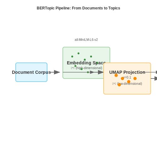
5.3 Real-Time Topic Monitoring
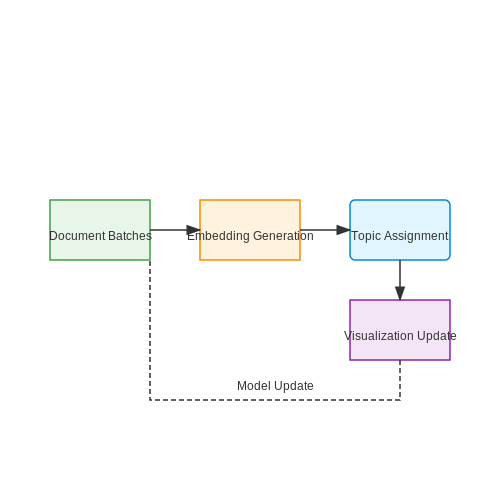
Real-time topic monitoring with BERTopic involves dynamically updating topic models as new documents stream in, enabling applications like social media trend analysis, customer feedback tracking, and live news aggregation. The core challenge lies in maintaining model consistency while adapting to evolving semantic distributions without full retraining.
Incremental Topic Modeling
BERTopic's online learning capability leverages the following components:
- Embedding Updates: New document embeddings are generated using the same sentence transformer, ensuring compatibility with existing topic representations.
- Cluster Evolution: HDBSCAN's approximate prediction mode assigns new documents to existing clusters or creates new ones based on cosine similarity thresholds.
- Topic Representation Maintenance: TF-IDF weighted c-TF-IDF vectors are recalculated incrementally using:
where Dt is the set of documents in topic t, ft,i is the frequency of term i in topic t, and N/nt is the inverse document frequency adjusted for topic prevalence.
Drift Detection and Adaptation
Semantic drift is monitored through:
- Topic Stability Scores: Measured via the Jensen-Shannon divergence between topic word distributions at time t and t+Δt:
where M = (P+Q)/2 and DKL is the Kullback-Leibler divergence. Thresholds above 0.3 typically trigger model revision.
- Novelty Detection: Outlier documents that fail to fit existing topics (HDBSCAN outlier scores > 0.9) are queued for periodic model updates.
Implementation Pipeline
The real-time processing workflow in BERTopic involves:
from bertopic import BERTopic
from sklearn.feature_extraction.text import CountVectorizer

# Initialize with online learning
topic_model = BERTopic(
    embedding_model="all-MiniLM-L6-v2",
    min_topic_size=15,
    vectorizer_model=CountVectorizer(stop_words="english"),
    calculate_probabilities=True
)

# Stream processing loop
for batch in document_stream:
    embeddings = topic_model.embedding_model.encode(batch)
    topics, probs = topic_model.topics_over_time(
        docs=batch,
        embeddings=embeddings,
        timestamps=[datetime.now()]*len(batch)
    )
    # Update visualization
    topic_model.visualize_topics_over_time()
Key parameters for optimization include min_topic_size (controls granularity), n_gram_range (for phrase detection), and nr_samples (for HDBSCAN's approximation quality).
Performance Considerations
Latency-critical deployments require:
- Embedding Caching: Reusing recent embeddings with LRU caches for similar documents
- Batch Processing: Optimal batch sizes (typically 50-100 docs) balance throughput and update frequency
- GPU Acceleration: Quantized transformer models like all-MiniLM-L6-v2 achieve 10ms inference times on T4 GPUs
6. Key Research Papers on BERTopic
6.1 Key Research Papers on BERTopic
- Topic Modeling with LSA, pLSA, LDA, NMF, BERTopic, Top2Vec: a ... — Image by author. Table of contents. Introduction; Topic Modeling Strategies 2.1 Introduction 2.2 Latent Semantic Analysis (LSA) 2.3 Probabilistic Latent Semantic Analysis (pLSA) 2.4 Latent Dirichlet Allocation (LDA) 2.5 Non-negative Matrix Factorization (NMF) 2.6 BERTopic and Top2Vec. Comparison; Additional remarks 4.1 A topic is not (necessarily) what we think it is 4.2 Topics are not easy to ...
- BERTopic: An Advanced Neural Topic Modeling Technique - Zilliz — Key Features of the BERTopic Model. The BERTopic model boasts several key features that make it a formidable tool for topic modeling: Modularity: BERTopic's modular design allows users to build their own topic model and experiment with several topic modeling techniques on top of their customized model. This flexibility enables users to tailor ...
- BERTopic: Neural topic modeling with a class-based TF-IDF procedure — Topic models can be useful tools to discover latent topics in collections of documents. Recent studies have shown the feasibility of approach topic modeling as a clustering task. We present BERTopic, a topic model that extends this process by extracting coherent topic representation through the development of a class-based variation of TF-IDF. More specifically, BERTopic generates document ...
- Optimizing BERTopic: Analysis and Reproducibility Study of ... - Springer — 1.1 Motivation for Reproducing BERTopic Experiments. Topic modeling is key in unsupervised text analysis, facilitating data exploration by uncovering latent topics. Topic modeling plays a pivotal role in information retrieval applications by automatically uncovering latent themes within vast text corpora, aiding in efficient document categorization and content recommendation.
- PDF Neural Topic Modeling with BERTopic: Submodel Selection Factors and ... — The benefits of topic modeling with that reach from use cases in market analysis, as well as in discovering themes in large textual data collections and papers. With the rising relevance of neural networks new possibilities arose, leading to the creation of neural topic models, which ingrain neural networks into topic modeling models.
- BERTopic: Neural topic modeling with a class-based TF ... - ResearchGate — 68 BERTopic modeling embedded with a pre-trained transformer model (e.g., HDBSCAN) and a c-TF-IDF method 68 can generate easily interpretable topics. BERTopic modeling was chosen over other topic ...
- arXiv:2203.05794v1 [cs.CL] 11 Mar 2022 — BERTopic: Neural topic modeling with a class-based TF-IDF procedure Maarten Grootendorst [email protected] Abstract Topic models can be useful tools to discover latent topics in collections of documents. Re-cent studies have shown the feasibility of ap-proach topic modeling as a clustering task. We present BERTopic, a topic model ...
- A Neural Topic Modelling framework for Guided Topic Extraction - Mathpix — It is a breakdown of the paper on the same topic by Maarten Grootendorst.. The article simplifies and tries to describe the novel state-of-the-art technique for topic modelling - BERTopic. ... Grootendorst M. "BERTopic: Neural topic modeling with a class-based TF-IDF procedure" (2022) Reimers N. et al. "Sentence-BERT: Sentence Embeddings using ...
- Neural topic modeling of machine learning applications in building: Key ... — In future, search keywords can be further refined by compiling an exhaustive variant of algorithm names. Moreover, ML application topics may not be comprehensively and accurately recognized due to uncertainties in neural topic models. Each step of the BERTopic model has some hyperparameters that may affect the topic-recognition results.
- An Enhanced BERTopic Framework and Algorithm for Improving Topic ... — In this paper, we enhance and customize the existing BERTopic framework to develop and implement an automated pipeline that delivers a more coherent and diverse set of topics with an even moderate ...
6.2 Recommended Books and Articles
- BERTopic:BERTopic: Neural topic modeling with a class-based TF-IDF ... — 5.2 Models. BERTopic will be compared to LDA, NMF, CTM, and Top2Vec. LDA and NMF were run through OCTIS with default parameters. The "all-mpnetbase-v2" SBERT model was used as the embedding model for BERTopic and CTM (Song et al., 2020). Two variations of Top2Vec were modeled, one with Doc2Vec and one with the "all-mpnet-base-v2" SBERT ...
- Topic Modeling with LSA, pLSA, LDA, NMF, BERTopic, Top2Vec: a ... — Image by author. Table of contents. Introduction; Topic Modeling Strategies 2.1 Introduction 2.2 Latent Semantic Analysis (LSA) 2.3 Probabilistic Latent Semantic Analysis (pLSA) 2.4 Latent Dirichlet Allocation (LDA) 2.5 Non-negative Matrix Factorization (NMF) 2.6 BERTopic and Top2Vec. Comparison; Additional remarks 4.1 A topic is not (necessarily) what we think it is 4.2 Topics are not easy to ...
- PDF Neural Topic Modeling with BERTopic: Submodel Selection Factors and ... — The benefits of topic modeling with that reach from use cases in market analysis, as well as in discovering themes in large textual data collections and papers. With the rising relevance of neural networks new possibilities arose, leading to the creation of neural topic models, which ingrain neural networks into topic modeling models.
- Iterative Improvement of an Additively Regularized Topic Model - Springer — Part of the book series: Lecture Notes in Computer Science ((volume 15419)) ... the final non-iterative model is the best model in terms of the number of good topics from the whole series. Topics with high coherence [2, ... BERTopic: neural topic modeling with a class-based TF-IDF procedure. arXiv preprint arXiv:2203.05794 (2022)
- Tutorial: Topic Modelling with BERTopic — By the end of this tutorial, you will be able to: Understand the Basics: Learn the fundamental concepts behind topic modeling and how BERTopic utilizes the BERT model to improve the accuracy and relevance of identified topics. Text Data Preprocessing: Discover best practices for preparing your text data for analysis. This includes data cleaning, preprocessing, and understanding how to format ...
- BERTopic: Neural topic modeling with a class-based TF-IDF procedure - ar5iv — To uncover common themes and the underlying narrative in text, topic models have proven to be a powerful unsupervised tool. Conventional models, such as Latent Dirichlet Allocation (LDA) (Blei et al., 2003) and Non-Negative Matrix Factorization (NMF) (Févotte and Idier, 2011), describe a document as a bag-of-words and model each document as a mixture of latent topics.
- Integration of Neural Embeddings and Probabilistic Models in Topic Modeling — BERTopic Embedding. In BERTopic, the process begins with generating document embeddings using pre-trained transformer-based language models like SBERT (Reimers and Gurevych Citation 2019).SBERT transforms sentences and documents into dense vector representations that capture semantic content, positioning semantically similar texts close in vector space.
- Neural topic modeling of machine learning applications in building: Key ... — Moreover, ML application topics may not be comprehensively and accurately recognized due to uncertainties in neural topic models. Each step of the BERTopic model has some hyperparameters that may affect the topic-recognition results. For instance, the pretrained transformer model "all-mpnet-base-v2" was selected to create document ...
- Leveraging spiking neural networks for topic modeling — The modern BERTopic model, which leverages a powerful language model based on multilayer transformer neural architecture, takes the lead on the remaining two datasets. It is worth noting, however, that a marginal difference can be observed between the STM and BERTopic models on the AG news dataset. This is an important observation because it ...
- (PDF) Topic Modeling: A Comprehensive Review - ResearchGate — After analysing approximately 300 research articles on topic modeling, a comprehensive survey on topic modelling has been presented in this paper. It includes classification hierarchy, Topic
6.3 Online Resources and Tutorials
- BERTopic:BERTopic: Neural topic modeling with a class-based TF-IDF ... — 5.2 Models. BERTopic will be compared to LDA, NMF, CTM, and Top2Vec. LDA and NMF were run through OCTIS with default parameters. The "all-mpnetbase-v2" SBERT model was used as the embedding model for BERTopic and CTM (Song et al., 2020). Two variations of Top2Vec were modeled, one with Doc2Vec and one with the "all-mpnet-base-v2" SBERT ...
- PDF Neural Topic Modeling with BERTopic: Submodel Selection Factors and ... — The benefits of topic modeling with that reach from use cases in market analysis, as well as in discovering themes in large textual data collections and papers. With the rising relevance of neural networks new possibilities arose, leading to the creation of neural topic models, which ingrain neural networks into topic modeling models.
- Tutorial: Topic Modelling with BERTopic — By the end of this tutorial, you will be able to: Understand the Basics: Learn the fundamental concepts behind topic modeling and how BERTopic utilizes the BERT model to improve the accuracy and relevance of identified topics. Text Data Preprocessing: Discover best practices for preparing your text data for analysis. This includes data cleaning, preprocessing, and understanding how to format ...
- Topic Modeling with LSA, pLSA, LDA, NMF, BERTopic, Top2Vec: a ... — Image by author. Table of contents. Introduction; Topic Modeling Strategies 2.1 Introduction 2.2 Latent Semantic Analysis (LSA) 2.3 Probabilistic Latent Semantic Analysis (pLSA) 2.4 Latent Dirichlet Allocation (LDA) 2.5 Non-negative Matrix Factorization (NMF) 2.6 BERTopic and Top2Vec. Comparison; Additional remarks 4.1 A topic is not (necessarily) what we think it is 4.2 Topics are not easy to ...
- BERTopic: Neural topic modeling with a class-based TF-IDF procedure - ar5iv — Topic models can be useful tools to discover latent topics in collections of documents. Recent studies have shown the feasibility of approach topic modeling as a clustering task. We present BERTopic, a topic model that extends this process by extracting coherent topic representation through the development of a class-based variation of TF-IDF.
- Implementation of Topic Modeling in the Analysis of Topic Trends in ... — This study employs topic modeling on data sourced from SemanticScholar using the BERTopic method, which captures the comprehensive context of research articles. ... The default BERTopic model, chosen as the optimal model, illustrates that there is a prevailing topic tendency in target 6.3 related to water quality. ... Electronic ISBN: 979-8 ...
- PDF MultiModalTopicExplorer: A Visual Text Analytics System for Exploring a ... — 2.2 BERTopic BERTopic [13] is a topic modeling technique that leverages Transform-ers and c-TF-IDF to create dense clusters allowing for easily inter-pretable topics whilst keeping important words in the topic descriptions. The algorithm can be split into three stages: 1. Embed documents: get document embeddings.
- An in-depth introduction to Topic Modeling using LDA and BERTopic — A variation of Bidirectional Encoder Representations from Transformers (BERT) has been developed to tackle topic modeling tasks. BERTopic was developed in 2020 by Grootendorst (2020) and is a ...
- Neural topic modeling of machine learning applications in building: Key ... — In future, search keywords can be further refined by compiling an exhaustive variant of algorithm names. Moreover, ML application topics may not be comprehensively and accurately recognized due to uncertainties in neural topic models. Each step of the BERTopic model has some hyperparameters that may affect the topic-recognition results.
- topic_models_BERTopic.ipynb - Colab - Google Colab — ['BAGHDAD, Iraq - A suicide attacker detonated a car bomb by police on a Baghdad bridge, and U.S. troops foiled a second suicide vehicle bombing in attacks Friday that killed at least five people and wounding at least 21...', ' BAGHDAD (Reuters) - At least 13 Iraqis were killed in a suicide car bomb attack on a major police checkpoint in central Baghdad on Friday, an Interior Ministry ...