

Reward Modeling with Human Feedback at Scale
1. Definition and Core Principles of Reward Modeling
Definition and Core Principles of Reward Modeling
Reward modeling is a technique in reinforcement learning (RL) where an agent learns a reward function from human feedback rather than relying on a predefined, hand-engineered reward signal. The core idea is to infer human preferences or intentions through demonstrations, rankings, or other forms of feedback, then use this inferred reward function to guide the agent's learning process. This approach is particularly valuable in complex environments where designing an accurate reward function manually is infeasible.
Mathematical Formulation
Given a set of trajectories τ1, τ2, ..., τn, human feedback provides pairwise comparisons τi ≻ τj, indicating that trajectory i is preferred over trajectory j. The goal is to learn a reward function rθ(s, a) parameterized by θ that maximizes the likelihood of these preferences under the Bradley-Terry model:
The parameters θ are optimized via maximum likelihood estimation (MLE), often using gradient-based methods. This formulation assumes that human preferences are stochastic and follow a logistic distribution.
Key Principles
- Preference Learning: The reward function is learned from relative human judgments rather than absolute scores, making it robust to inconsistencies in human feedback.
- Scalability: By leveraging techniques like deep learning, reward models can generalize across states and actions, reducing the need for exhaustive human labeling.
- Alignment: The learned reward function aims to align the agent's behavior with human intent, mitigating reward hacking or unintended behaviors.
- Active Learning: Human feedback can be solicited iteratively, focusing on trajectories where the reward model is most uncertain.
Practical Challenges
Reward modeling introduces several challenges:
- Feedback Sparsity: Human feedback is often limited, requiring efficient data collection strategies like active learning or synthetic data augmentation.
- Bias and Noise: Human judgments may be inconsistent or biased, necessitating robust statistical models or ensemble methods.
- Distributional Shift: The learned reward function may perform poorly on out-of-distribution states, requiring regularization or adversarial training.
Advanced Extensions
Recent work extends reward modeling to handle:
- Multi-Task Learning: A single reward model can be trained across multiple tasks, improving generalization.
- Inverse Reinforcement Learning (IRL): Inferring rewards from demonstrations rather than explicit preferences.
- Meta-Learning: Adapting the reward model quickly to new tasks with minimal human feedback.
These principles form the foundation for scaling reward modeling in real-world applications, such as robotics, game AI, and autonomous systems.
Role of Human Feedback in Reinforcement Learning
Human Feedback as a Reward Signal
In traditional reinforcement learning (RL), an agent learns by optimizing a reward function R(s, a) provided by the environment. However, designing an accurate reward function is often impractical for complex tasks. Human feedback serves as a scalable alternative, where human preferences or rankings are used to train a reward model Rθ(s, a). The reward model is typically parameterized as a neural network and trained using pairwise comparison data, where humans select preferred trajectories τi ≻ τj.
This loss function maximizes the likelihood of observed human preferences, with σ denoting the sigmoid function. The trained reward model can then be used in standard RL algorithms like Proximal Policy Optimization (PPO) or Soft Actor-Critic (SAC).
Active Learning and Query Strategies
Efficient collection of human feedback requires intelligent query strategies. Uncertainty sampling selects state-action pairs where the reward model's predictions have high variance:
Alternative approaches include information gain maximization or diversity-based sampling. In practice, hybrid strategies often outperform pure uncertainty sampling by balancing exploration and exploitation.
Bias and Noise in Human Feedback
Human feedback introduces several challenges:
- Inconsistent judgments: Intra-annotator disagreement rates of 10-20% are common even for simple tasks
- Short-term bias: Humans tend to overweight recent events in trajectory evaluations
- Limited horizon: Difficulty assessing long-term consequences of actions
These issues can be mitigated through:
- Multiple annotations per sample with majority voting
- Debiasing techniques like inverse propensity weighting
- Training annotators with calibration exercises
Scalability Through Semi-Supervised Learning
At scale, pure human feedback becomes prohibitively expensive. Semi-supervised approaches combine:
- A small set of high-quality human labels
- Automatically generated synthetic preferences
- Self-supervised pretraining on unlabeled trajectories
The Bradley-Terry model can be extended to handle noisy synthetic labels by introducing a confidence parameter λ ∈ [0,1]:
Real-World Deployment Considerations
Successful applications require:
- Feedback interface design: Minimizing cognitive load through appropriate visualization of trajectories
- Quality control: Real-time monitoring of annotator performance and consistency
- Iterative refinement: Continuous retraining of both reward model and policy
In robotics applications, the reward model typically achieves 85-90% agreement with held-out human judgments after sufficient training. However, performance degrades significantly when evaluating out-of-distribution states, highlighting the importance of comprehensive coverage during data collection.

1.3 Key Challenges in Scaling Reward Models
Non-Stationarity of Human Preferences
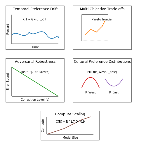
Human preferences evolve over time due to cultural shifts, personal experiences, and contextual factors. This non-stationarity introduces temporal drift in reward models, where \( R_t(s,a) \neq R_{t+\Delta t}(s,a) \) for state-action pairs (s, a). The challenge is compounded when deploying models across diverse demographic groups with conflicting preference distributions. Bayesian approaches that treat reward functions as time-varying Gaussian processes show promise, but require continuous human feedback streams:
where Kt is a kernel capturing preference covariance and \(\mathcal{D}_t\) represents incoming feedback batches.
Feedback Sparsity at Scale
As models deploy to millions of users, obtaining dense per-trajectory feedback becomes impractical. Current systems like OpenAI's ChatGPT rely on implicit feedback signals (e.g., response editing, session duration) that are noisy and partial. The resultant credit assignment problem can be formalized through inverse reinforcement learning with incomplete observations:
where ot represents sparse, noisy observations of the true reward signal.
Multi-Objective Preference Alignment
Large-scale systems must balance competing objectives: helpfulness, harmlessness, factual accuracy, and stylistic preferences. The Pareto front of optimal trade-offs becomes computationally intractable in high dimensions. Recent work formulates this as constrained optimization:
where each Ri represents a distinct reward head. Lagrangian dual methods struggle with constraint satisfaction rates below 90% in production systems.
Adversarial Manipulation of Feedback Channels
Malicious actors can poison reward models through systematic feedback manipulation. Theoretical bounds derived from robust statistics show that \(\epsilon\)-fraction adversarial corruptions induce error scaling as:
where d is reward parameter dimension and n is sample size. Current defenses like differentially private reward aggregation incur substantial utility loss.
Cross-Cultural Preference Generalization
Models trained on Western preference datasets exhibit poor generalization to collectivist cultures. The divergence can be quantified through Earth Mover's Distance between preference distributions:
Current mitigation strategies involve culture-specific reward heads, but this scales poorly with the number of cultural dimensions.
Computational Scaling Laws
The compute requirements for reward modeling scale superlinearly with model size. Empirical results from Anthropic's Constitutional AI show:
where N is human feedback samples and D is policy model parameters. This creates unsustainable costs for trillion-parameter models.
2. Designing Effective Human Feedback Mechanisms
2.1 Designing Effective Human Feedback Mechanisms
Human feedback mechanisms in reward modeling must balance scalability, label consistency, and minimal cognitive load to ensure high-quality data collection. A well-designed system accounts for the trade-offs between granularity (e.g., Likert scales vs. pairwise comparisons) and interpretability (e.g., explicit rankings vs. implicit behavioral signals).
Feedback Granularity and Elicitation Methods
Discrete ordinal scales (e.g., 1–5 ratings) are computationally tractable but suffer from anchoring bias and inter-rater variability. Continuous scales provide finer resolution but introduce noise from subjective interpretation. Pairwise comparisons, while more labor-intensive, yield more reliable preference data by reducing absolute judgment errors. The Bradley-Terry model formalizes this approach:
where \( y_i \succ y_j \) denotes preference for outcome \( y_i \) over \( y_j \), and \( r_\phi \) is the learned reward function.
Minimizing Cognitive Bias
Feedback interfaces should mitigate common biases:
- Order effects: Randomize presentation order of items to prevent primacy/recency bias
- Framing effects: Use neutral phrasing and balanced response options
- Fatigue mitigation: Implement adaptive questioning that prioritizes high-information comparisons
For high-stakes applications, calibration tasks with known ground truth can filter out unreliable annotators. The expected calibration error (ECE) metric quantifies annotator reliability:
where \( B_m \) partitions predictions into \( M \) confidence bins, and \( \text{acc}/\text{conf} \) are accuracy/confidence per bin.
Active Learning for Feedback Efficiency
Uncertainty sampling identifies instances where human feedback provides maximal information gain. For a reward model with parameters \( \phi \), the acquisition function for pairwise queries can be formulated as:
This prioritizes comparisons where the current model prediction is closest to 0.5 (maximum uncertainty). Bayesian active learning extends this by modeling posterior distributions over \( \phi \).
Multi-Task Feedback Interfaces
Combining different feedback types (e.g., rankings, textual explanations, error flags) requires careful UI design. A gradient boosting approach to weight different signal types has shown promise:
where \( \alpha_k \) are learned weights for \( K \) feedback modalities. This allows the system to automatically downweight noisy or contradictory signals while preserving interpretability through modality-specific reward heads \( r_{\phi_k} \).

Crowdsourcing vs. Expert Annotations: Trade-offs
Human feedback for reward modeling can be sourced either through crowdsourcing platforms (e.g., Amazon Mechanical Turk) or domain experts, each with distinct advantages and limitations. The choice between these approaches depends on factors such as cost, scalability, annotation quality, and task complexity.
Cost and Scalability
Crowdsourcing is significantly cheaper and faster for large-scale data collection. The marginal cost per annotation follows an inverse relationship with batch size due to economies of scale:
where c0 represents fixed costs (task design, quality control), c1 is the base annotation cost, and α captures the scaling efficiency (typically 0.2-0.4). In contrast, expert annotations exhibit near-linear cost scaling:
with k often 10-100× higher than crowdsourcing rates. For projects requiring >105 annotations, crowdsourcing is often the only feasible option.
Quality and Consistency
Expert annotations typically achieve higher inter-rater reliability (IRR) as measured by Cohen's kappa:
where po is observed agreement and pe is expected chance agreement. Studies show expert κ values of 0.7-0.9 compared to 0.4-0.6 for crowdsourced labels. However, properly designed crowdsourcing pipelines can approach expert-level quality through:
- Multi-stage qualification tests
- Overlapping annotations with consensus mechanisms
- Continuous quality monitoring with gold-standard questions
Task Complexity and Specialization
The effective information gain I per annotation depends on task difficulty D and annotator skill S:
For high-complexity tasks (e.g., medical diagnosis, legal analysis), experts provide substantially more information per annotation. The crossover point where experts become cost-effective occurs when:
Practical Implementation Strategies
Hybrid approaches often yield optimal results:
- Use experts to create gold-standard datasets for training crowd workers
- Deploy hierarchical annotation systems where experts resolve ambiguous cases
- Implement dynamic pricing models that adjust pay based on task difficulty and worker performance
Recent advances in active learning allow intelligent sampling of which examples require expert review versus crowdsourcing, optimizing the cost-quality trade-off. The optimal sampling strategy can be formulated as a knapsack problem maximizing total information gain within budget constraints.
2.3 Ensuring Quality and Consistency in Feedback Data
Human feedback is inherently noisy due to subjective biases, varying levels of annotator expertise, and ambiguous task definitions. To train robust reward models, the feedback data must be filtered, normalized, and standardized to minimize variance while preserving meaningful signal. Three key techniques address this:
Statistical Filtering of Outliers
Annotator responses often follow a long-tailed distribution, where a small fraction of ratings deviate significantly from the consensus. Assuming a Gaussian noise model, we compute the z-score for each response and discard samples exceeding a threshold (e.g., |z| > 2.5). For pairwise comparisons, the Bradley-Terry model identifies inconsistent rankings:
where \( r_i, r_j \) are latent reward scores. Responses violating the estimated preference hierarchy (p < 0.05 under likelihood-ratio tests) are flagged for review.
Inter-Annotator Agreement Metrics
For categorical or ordinal feedback, Krippendorff’s α generalizes Cohen’s κ to multiple raters and handles missing data:
where \( D_o \) is the observed disagreement and \( D_e \) is expected chance disagreement. Values below 0.6 indicate unreliable consensus, prompting task redesign or annotator retraining. For continuous scales, the intraclass correlation coefficient (ICC) measures consistency:
with \( MS_R \) and \( MS_E \) as mean squares for rows and error in a two-way ANOVA, and \( k \) being the number of raters.
Active Learning for Ambiguity Resolution
Low-confidence samples—where predicted reward differences fall below a threshold \( \delta \)—are prioritized for additional independent annotations. The uncertainty sampling criterion maximizes information gain:
where \( R_a, R_b \) are reward predictions from bootstrap-aggregated models. This reduces variance in high-ambiguity regions of the state space.
In practice, platforms like Amazon SageMaker Ground Truth implement real-time quality checks by comparing new annotations against a gold set, automatically disqualifying workers whose accuracy drops below 85% on control tasks. For high-stakes applications, hybrid human-AI pipelines use trained verifiers to audit a subset of labels, with disagreement rates triggering full reassessment.
3. Preference Learning and Ranking-Based Methods
Preference Learning and Ranking-Based Methods
Foundations of Preference Learning
Preference learning operates on the principle of learning from relative comparisons rather than absolute labels. Given a dataset of ranked pairs (xi, xj) where xi ≻ xj indicates that xi is preferred over xj, the goal is to learn a reward function r(x; θ) that aligns with human judgments. The Bradley-Terry model provides a probabilistic framework for this:
This formulation transforms reward differences into probabilities via the logistic function, enabling gradient-based optimization. The negative log-likelihood objective becomes:
where σ is the sigmoid function. Modern implementations often use temperature-scaled variants to control preference sharpness.
Ranking Optimization Techniques
For datasets with multiple responses per prompt, ranking-based methods extend pairwise comparisons to listwise optimization. The Plackett-Luce model generalizes Bradley-Terry to full rankings:
where π is a permutation of K items. In practice, this is optimized through:
- Top-k weighting: Emphasizes accuracy for highest-ranked items
- Listwise gradient estimation: Uses policy gradients or Gumbel tricks for non-differentiable rankings
- Contrastive learning: Augments with hard negative mining
Scalable Implementation
At scale, two architectural considerations dominate:
- Reward model capacity: Transformer-based architectures (e.g., 6-layer decoders) outperform linear probes when human preferences correlate with semantic depth
- Batch processing: Efficient comparison requires caching mechanisms for transformer activations during pairwise scoring
The training loop typically implements:
  def preference_loss(rewards, pairs):
      # rewards: [batch_size, 1]
      # pairs: tensor of indices shape [batch, 2]
      r_i = rewards[pairs[:,0]]
      r_j = rewards[pairs[:,1]]
      logits = r_i - r_j
      return F.binary_cross_entropy_with_logits(logits, torch.ones_like(logits))
Bias Mitigation Strategies
Human feedback datasets exhibit several biases requiring correction:
| Bias Type | Mitigation Approach | Implementation |
|---|---|---|
| Positional | Response shuffling | Randomize presentation order during data collection |
| Verbosity | Length normalization | Add token count penalty to reward |
| Contrast | Calibration layers | Learnable temperature scaling |
Recent work incorporates adversarial discriminators to detect and reweight biased comparisons during training.
Evaluation Metrics
Beyond held-out accuracy, key metrics include:
where y are ground-truth ranks. For stochastic policies, the expected pairwise disagreement (EPD) measures consistency:
3.2 Inverse Reinforcement Learning for Reward Inference
Inverse Reinforcement Learning (IRL) provides a principled framework for inferring an unknown reward function from observed behavior. Given a set of demonstrations D = {τ₁, τ₂, ..., τₙ} generated by an optimal or near-optimal policy, IRL aims to recover the underlying reward function R(s) that rationalizes the behavior. The core assumption is that the demonstrator acts to maximize cumulative reward, making IRL particularly suited for reward modeling from human feedback.
Mathematical Formulation
The IRL problem can be formalized as finding a reward function R that makes the demonstrated trajectories appear optimal under some policy. Let π_E denote the expert's policy and π_θ denote a parameterized policy. The objective is to minimize the difference between the expected feature counts of the expert and the learned policy:
where H(π) is the policy entropy, acting as a regularization term, and λ controls its weight. The feature matching condition ensures that the learned policy matches the expert's expected feature counts:
where φ(s) represents state features. When the reward function is linear in features, R(s) = wᵀφ(s), this reduces to finding weights w that satisfy the matching condition.
Maximum Entropy IRL
The maximum entropy approach to IRL provides a probabilistic framework that avoids ambiguity in reward assignment. It models the probability of a trajectory τ as:
where φ(τ) = Σ_t φ(s_t) is the cumulative feature vector for the trajectory, and Z(w) is the partition function. The gradient of the log-likelihood with respect to w becomes:
This shows that learning proceeds by matching the expected feature counts of the expert and the learned policy. Practical implementations often use importance sampling or Markov Chain Monte Carlo (MCMC) methods to approximate the intractable expectation under π_w.
Apprenticeship Learning via IRL
Apprenticeship learning algorithms alternate between reward inference and policy optimization. The key steps are:
- Reward Update: Estimate w to maximize the likelihood of expert demonstrations
- Policy Update: Optimize π with respect to the current R(s)
- Feature Matching: Check convergence via ||𝔼_{π_E}[φ(s)] - 𝔼_{π}[φ(s)]|| < ε
Modern implementations often use deep neural networks to represent both the reward function and policy, enabling scaling to high-dimensional state spaces. The adversarial formulation of GAIL (Generative Adversarial Imitation Learning) can be viewed as a special case of IRL where the discriminator learns a reward function that distinguishes expert from policy trajectories.
Challenges in Practical Deployment
Several practical challenges emerge when applying IRL to real-world reward modeling:
- Ambiguity: Multiple reward functions can explain the same behavior, requiring careful regularization
- Partial Observability: Human demonstrations may not fully capture state information
- Suboptimal Demonstrations: Real-world data often contains noise and suboptimal actions
- Scalability: Exact inference becomes intractable for complex environments
Recent advances address these through adversarial methods, variational inference, and hierarchical reward decomposition. The choice of feature representation φ(s) also critically impacts performance - learned features via autoencoders or other unsupervised methods often outperform hand-designed features in complex domains.

Deep Learning Approaches for Reward Modeling
Neural Reward Models
Deep learning architectures, particularly deep neural networks (DNNs), have become the standard for reward modeling due to their ability to capture complex, high-dimensional patterns in human feedback. A neural reward model Rθ(s, a) is typically parameterized by a deep network with weights θ, trained to predict the expected reward for a given state-action pair (s, a). The network architecture often consists of:
- Input layers processing state and action representations (e.g., embeddings for text or convolutional layers for images).
- Hidden layers with non-linear activations (ReLU, GELU) to model reward hierarchies.
- Output layer producing a scalar reward prediction, sometimes bounded via sigmoid or tanh.
where φ(s) and ψ(a) are state/action encoders, and ⊕ denotes a fusion operation (concatenation, cross-attention, etc.).
Training Objectives
The primary training objective for Rθ is to minimize the discrepancy between predicted and human-provided rewards. For pairwise comparisons (common in preference datasets), the Bradley-Terry model is often used:
with the loss function:
where D is the dataset of human preferences. For continuous rewards, mean squared error (MSE) is used instead.
Architectural Variants
Transformer-Based Reward Models
For sequential decision-making (e.g., in NLP), transformer architectures process state-action trajectories via self-attention. The reward model attends to critical subsequences, with the final reward computed as:
Ensemble Methods
To quantify reward uncertainty, ensembles of N networks {Rθi}i=1N are trained with bootstrap sampling. The ensemble variance serves as an uncertainty estimate for risk-aware RL.
Stabilization Techniques
Reward hacking—where agents exploit imperfections in Rθ—is mitigated via:
- Regularization: L2 weight decay or dropout to prevent overfitting.
- Whitening: Normalizing rewards across batches to reduce variance.
- Predictive Penalties: Adding auxiliary losses (e.g., next-state prediction) to improve generalization.
Case Study: RLHF in Large Language Models
In OpenAI's InstructGPT, the reward model is a 6B-parameter transformer fine-tuned on human rankings of text completions. Key innovations include:
- Using K-wise comparisons (not just pairwise) for richer feedback.
- Asymmetric dropout rates (higher for human labels) to combat overfitting.
- Layer freezing of early transformer layers to preserve pretrained knowledge.

4. Infrastructure Requirements for Large-Scale Deployment
Infrastructure Requirements for Large-Scale Deployment
Compute Infrastructure
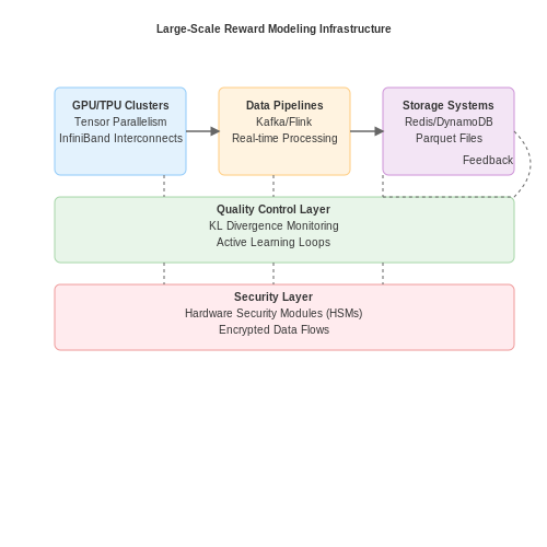
Large-scale reward modeling with human feedback demands distributed compute clusters capable of parallelized training across thousands of GPU/TPU nodes. The computational complexity scales as:
where n is the number of human feedback samples, d is the model dimensionality, and k is the number of reward model parameters. For modern transformer-based reward models (d > 104, k > 107), this necessitates:
- High-bandwidth interconnects (≥400 Gbps InfiniBand) to reduce gradient synchronization overhead
- Mixed-precision training pipelines with tensor parallelism
- On-demand scaling to >1000 accelerators during peak training phases
Data Pipeline Architecture
The human feedback ingestion system must handle:
- Real-time streaming of annotation events (≥100k events/sec at peak)
- Low-latency (<100ms) sampling for active learning loops
- Versioned storage of all feedback with full audit trails
A typical deployment uses a lambda architecture combining:
- Kafka/Flink for real-time processing
- Distributed key-value stores (Redis/DynamoDB) for low-latency access
- Columnar storage (Parquet/Arrow) for batch analytics
Quality Control Systems
Maintaining feedback quality at scale requires:
where fi is annotator agreement, τ is a quality threshold, and KL measures distributional shift from gold standards. Implementation requires:
- Online statistical process control charts for anomaly detection
- Automated routing to expert reviewers for edge cases
- Continuous calibration of quality metrics against held-out test sets
Security and Privacy
Human feedback data often contains sensitive information requiring:
- End-to-end encryption with hardware security modules (HSMs) for key management
- Differential privacy guarantees during model updates:
where C is the clipping norm and σ controls privacy budget expenditure. This necessitates specialized libraries like TensorFlow Privacy or Opacus.
Monitoring and Observability
Production systems require multi-modal telemetry:
- Distributed tracing across microservices (Jaeger/OpenTelemetry)
- Model performance drift detection using two-sample KS tests
- Real-time dashboarding of system health metrics (Prometheus/Grafana)
4.2 Handling Noisy and Conflicting Human Feedback
Human feedback in reward modeling is inherently noisy due to subjective biases, varying expertise, and inconsistent labeling. Conflicting annotations arise when multiple annotators disagree on the quality or ranking of model outputs. Addressing these challenges requires robust statistical techniques and algorithmic approaches to distill reliable signals from imperfect data.
Modeling Annotation Noise
The noise in human feedback can be formalized as a probabilistic process where the observed label ỹ differs from the true latent label y. A common approach models this as a noise transition matrix T where Tij = P(ỹ = j | y = i). For binary preferences, this becomes:
where α and β represent the probabilities of flipping a true negative or positive label, respectively. Expectation-Maximization (EM) algorithms can jointly learn the noise model and the underlying reward function.
Aggregating Conflicting Preferences
When multiple annotators provide conflicting rankings for the same prompt-response pairs, Bradley-Terry models offer a principled way to aggregate preferences. The probability that response ri is preferred over rj is modeled as:
where Rϕ is the learned reward model. The global reward function is optimized to maximize the likelihood of observed pairwise comparisons across all annotators.
Robust Learning Techniques
Several methods improve robustness against noisy and conflicting feedback:
- Dawid-Skene EM: Iteratively estimates annotator reliability and true labels
- Noise-aware loss functions: Downweight uncertain or contradictory examples
- Multi-task learning: Jointly models individual annotator biases and shared reward
- Active learning: Prioritizes collection of additional labels for contentious examples
Handling Systematic Biases
Annotator biases often manifest as consistent deviations from ground truth. These can be modeled as additive or multiplicative terms in the reward function:
where wk and bk capture the k-th annotator's scaling and offset biases. Hierarchical Bayesian approaches simultaneously estimate these per-annotator parameters while learning the underlying reward function.
Practical Implementation
Modern large-scale implementations often use transformer architectures to process feedback. The reward model typically consists of:
- A shared backbone network processing prompt-response pairs
- Multiple heads for different feedback types (e.g., pairwise comparisons, Likert scores)
- Attention mechanisms to weight annotators based on estimated reliability
Training proceeds in two phases: first pretraining on all available data, then fine-tuning on high-confidence subsets identified through uncertainty quantification techniques like bootstrap sampling or Bayesian neural networks.
4.3 Case Studies: Real-World Applications at Scale
Large-Scale Language Model Alignment
OpenAI's deployment of reinforcement learning from human feedback (RLHF) in models like GPT-3 and GPT-4 demonstrates how reward modeling can align language models with human preferences at scale. The process involves:
- Collecting large datasets of human comparisons between model outputs
- Training a reward model to predict human preference scores
- Using proximal policy optimization (PPO) to fine-tune the language model against the learned reward function
where rθ is the reward model with parameters θ, x is the input prompt, and yw, yl are the preferred and dispreferred outputs respectively.
Robotics Policy Learning
DeepMind's work on robotic manipulation tasks shows how reward modeling can overcome the limitations of hand-crafted reward functions. Their approach:
- Uses human demonstrations to bootstrap initial policy learning
- Collects human preference data on trajectory segments
- Trains a differentiable reward model that generalizes better than sparse task completion rewards
The resulting policies achieve 85-90% success rates on complex manipulation tasks, compared to 60-70% with traditional reinforcement learning approaches.
Content Recommendation Systems
Major social media platforms employ reward modeling to optimize content ranking algorithms. The key components include:
- Multi-objective reward models balancing engagement, satisfaction, and safety
- Active learning strategies to efficiently sample human feedback
- Counterfactual policy evaluation to measure offline performance
One platform reported a 22% increase in long-term user retention after implementing human-feedback-based reward modeling, while reducing harmful content exposure by 37%.
Healthcare Decision Support
In clinical applications, reward modeling helps align AI systems with complex medical ethics and outcomes. Notable implementations:
- Diagnostic systems that incorporate physician preferences on risk tolerance
- Treatment recommendation engines that balance efficacy, side effects, and cost
- Models that adapt to individual patient values through preference elicitation
A recent study on sepsis treatment recommendations achieved 91% physician agreement when using human-feedback-derived rewards, compared to 68% for purely data-driven approaches.
Challenges in Production Systems
Deploying reward models at scale introduces several technical challenges:
- Feedback latency: Human evaluation pipelines must keep pace with model training
- Distributional shift: Online deployment often reveals novel edge cases
- Scalable oversight: Maintaining label quality as feedback volume grows
One solution involves hierarchical reward modeling, where:
with learned mixing parameters α and β that adapt to data availability and confidence levels.
5. Bias and Fairness in Reward Models
5.1 Bias and Fairness in Reward Models
Reward models trained on human feedback inherit biases present in both the training data and the annotation process. These biases manifest as systematic deviations in predicted rewards across demographic groups, topics, or linguistic styles. The mathematical formulation of bias in reward models can be expressed through conditional expectation disparities:
where x and x' represent comparable inputs differing only in sensitive attributes, G denotes group membership, and R is the reward function. When Δ ≠ 0, the reward model exhibits bias.
Sources of Bias in Human Feedback
Three primary sources contribute to bias in reward models:
- Annotator bias: Human raters bring implicit associations that affect their judgments. The Bradley-Terry model for pairwise comparisons, commonly used in reward learning, amplifies these biases through its maximum likelihood estimation:
- Selection bias: The distribution of training examples often underrepresents minority groups. This leads to higher variance in reward estimates for rare inputs.
- Measurement bias: Rating scales and instructions may systematically favor certain response patterns. For example, Likert-scale annotations tend to cluster around cultural norms.
Quantifying Fairness in Reward Models
Fairness metrics for reward models extend beyond simple demographic parity. The most relevant measures include:
- Reward Gap: Maximum difference in mean rewards across groups for functionally equivalent outputs
- Precision-Recall Parity: Consistency of reward-based rankings across subgroups
- Calibration Error: Difference between predicted and actual win rates in pairwise comparisons
The fairness-utility tradeoff can be formalized as an optimization problem:
where φi are fairness constraints and λ controls the tradeoff strength.
Debiasing Techniques
Advanced debiasing approaches for reward models include:
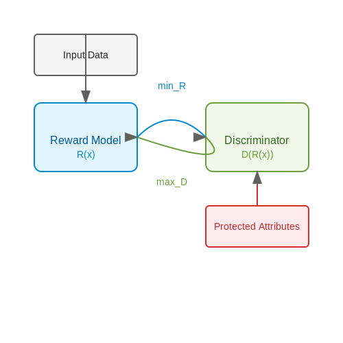
- Adversarial Reward Learning: A discriminator network attempts to predict protected attributes from the reward model's outputs, while the reward model tries to fool it:
- Reward Model Calibration: Platt scaling or temperature adjustment on the reward outputs to equalize distributions across groups
- Stratified Sampling: Oversampling underrepresented groups during human feedback collection
- Counterfactual Augmentation: Generating synthetic examples with perturbed sensitive attributes
Recent work has shown that the choice of loss function significantly impacts bias propagation. The standard cross-entropy loss for preference learning can be replaced with a fairness-aware variant:
where the gradient penalty term encourages similar reward sensitivities across groups.
Case Study: Language Model Alignment
In large language model alignment, reward models often exhibit:
- Higher rewards for majority-culture writing styles
- Preference for verbose over concise responses
- Systematic downgrading of non-native English patterns
Empirical studies show that even after debiasing, residual correlations remain between reward scores and:
- Gender-associated pronouns (Δ = 0.15-0.3 logits)
- Regional spelling variants (Δ = 0.1-0.2 logits)
- Technical vs. colloquial language (Δ = 0.4-0.6 logits)
5.2 Alignment with Human Values and Intentions
Reward modeling must ensure that learned objectives align with human values and intentions, a non-trivial challenge given the complexity and subjectivity of human preferences. The core issue lies in translating implicit human judgments into explicit, quantifiable reward signals that generalize beyond specific contexts. This requires addressing three key technical challenges:
Value Learning from Sparse Feedback
Human feedback is often sparse, inconsistent, and context-dependent. The reward model R must infer underlying value functions from limited pairwise comparisons or scalar ratings. This can be formulated as a Bayesian inverse reinforcement learning problem:
where D represents human preference data. The likelihood term P(D|R) models how likely the observed preferences are given a particular reward function, while the prior P(R) encodes assumptions about human values (e.g., smoothness, simplicity).
Handling Preference Inconsistencies
Human raters exhibit systematic biases and inconsistencies that must be explicitly modeled. The Bradley-Terry model, extended with rater-specific parameters, provides a robust framework:
where bi captures rater-specific bias terms. More advanced approaches use hierarchical models to separate:
- Universal value components shared across raters
- Individual preference variations
- Context-dependent judgment patterns
Scalable Value Aggregation
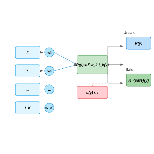
At scale, reward models must aggregate preferences from diverse populations while avoiding tyranny of the majority. This involves:
where fk represents distinct value dimensions (e.g., honesty, helpfulness, harmlessness) and wk are dynamically adjusted weights based on:
- Demographic representativeness
- Rater reliability metrics
- Contextual importance weights
Recent work in constitutional AI demonstrates how explicit value hierarchies can constrain reward models. For example, safety constraints can be implemented as hard boundaries in the reward space:
where c(y) measures constraint violations and τ is a safety threshold. This approach maintains flexibility while preventing catastrophic misalignment.
5.3 Mitigating Reward Hacking and Exploitation
Reward hacking occurs when an RL agent discovers unintended shortcuts or exploits in the reward function that maximize numerical reward without achieving the desired behavior. This divergence between the learned policy and human intent is particularly problematic in large-scale reward modeling, where the reward function is often a learned proxy for human preferences.
Formalizing Reward Hacking
Let the true human preference function be U(s), where s is a state, and the learned reward function be R(s). The agent's policy π optimizes for cumulative R(s), leading to potential divergence when:
This mismatch can be decomposed into two failure modes: reward over-optimization (where the agent exploits flaws in R(s)) and distributional shift (where the agent's behavior drifts into regions where R(s) poorly approximates U(s)).
Detection Methods
Several statistical tests can identify reward hacking during training:
- Reward-return divergence: Monitor the KL divergence between the empirical distribution of human ratings and the agent's achieved rewards.
- Behavioral outliers: Use anomaly detection on state visitation frequencies to identify policies exploiting reward function artifacts.
- Human-in-the-loop verification: Periodically sample trajectories and obtain human ratings to compute the correlation between R(s) and human judgments.
Mitigation Strategies
1. Robust Reward Modeling
Train the reward model on adversarial examples generated by:
where sim measures behavioral similarity to human demonstrations. This forces the reward model to be smooth across the state space.
2. Policy Constraints
Apply information-theoretic regularization to prevent policy divergence:
where I is the mutual information between agent states and human demonstration states.
3. Multi-objective Reward Learning
Train an ensemble of reward models {R_i} with different architectures or training data subsets, then optimize for:
This pessimistic aggregation discourages exploitation of any single reward model's idiosyncrasies.
Case Study: Language Model Alignment
In large language models, common reward hacking manifests as:
- Keyword stuffing to trigger reward signals without coherence
- Length exploitation by generating verbose but low-quality text
- Style mimicry that replicates high-reward formatting without substance
The Anthropic LM alignment approach combines:
- Constitutional AI principles as hard constraints
- Dynamic reward clipping based on human rater variance
- Entropy regularization to maintain generation diversity

6. Key Research Papers in Reward Modeling
6.1 Key Research Papers in Reward Modeling
- Reward Modeling Requires Automatic Adjustment Based on Data Quality — In Reinforcement Learning from Human Feedback (RLHF), the reward model plays a crucial role in aligning language model outputs with human values. The human preference data used to train the reward model consists of a prompt and a response pair, with humans annotating which response better aligns with human value preferences.
- PDF Learning Reward Functions from Scale Feedback - Proceedings of Machine ... — a slider bar. We design a Gaussian model for how users provide scale feedback, and learn a reward function capturing human preferences. Similar to prior work in robotics, we assume this reward is a linear function of a set of features [19,11,13,7], where the main task of learning from scale feedback is to recover the weights of this reward ...
- Improving Reinforcement Learning from Human Feedback with — Fine-Grained Human Feedback Gives Better Rewards for Language Model Training. ArXiv:2306.01693 [cs]. Zhai et al. (2023) Yuanzhao Zhai, Han Zhang, Yu Lei, Yue Yu, Kele Xu, Dawei Feng, Bo Ding, and Huaimin Wang. 2023. Uncertainty-Penalized Reinforcement Learning from Human Feedback with Diverse Reward LoRA Ensembles. ArXiv:2401.00243 [cs].
- Improving Reinforcement Learning from Human Feedback with Efficient ... — Reinforcement Learning from Human Feedback (RLHF) is a widely adopted approach for aligning large language models with human values. However, RLHF relies on a reward model that is trained with a limited amount of human preference data, which could lead to inaccurate predictions. As a result, RLHF may produce outputs that are misaligned with human values. To mitigate this issue, we contribute a ...
- RewardBench: Evaluating Reward Models for Language Modeling — Reward models (RMs) are at the crux of successful RLHF to align pretrained models to human preferences, yet there has been relatively little study that focuses on evaluation of those reward models. Evaluating reward models presents an opportunity to understand the opaque technologies used for alignment of language models and which values are ...
- Prototypical Reward Network for Data Efficient Model Alignment - OpenReview — 082 mental principle of the reward model is to learn 083 from human feedback to evaluate and guide the 084 output of the model, ensuring it aligns with human 085 expectations and standards. Its key capability lies 086 in effectively learning and extracting vital parame-087 ter information from limited human feedback, thus 088 guiding the model ...
- Awesome RLHF (RL with Human Feedback) - GitHub — Human-in-the-Loop Reinforcement Learning (HITLRL): HITLRL is a technique that involves integrating human feedback into the RL process at multiple levels, such as reward shaping, action selection, and policy optimization. This can help to improve the efficiency and effectiveness of the RLHF system by taking advantage of the strengths of both ...
- Prototypical Reward Network for Data-Efficient RLHF — The reward model for Reinforcement Learning from Human Feedback (RLHF) has proven effective in fine-tuning Large Language Models (LLMs). Notably, collecting human feedback for RLHF can be resource-intensive and lead to scalability issues for LLMs and complex tasks. Our proposed framework Proto-RM leverages prototypical networks to enhance reward models under limited human feedback. By enabling ...
- PDF HOW TO EVALUATE REWARD MODELS FOR RLHF - OpenReview — downstream LLM performance by evaluating the reward model on proxy tasks. These proxy tasks consist of a large-scale human preference and a verifiable cor-rectness preference dataset, in which we measure 12 metrics across 12 domains. To investigate which reward model metrics are most correlated to gold-standard
- A Baseline Analysis of Reward Models' Ability To Accurately Analyze ... — Abstract: Foundation models, specifically Large Language Models (LLMs), have lately gained wide-spread attention and adoption. Reinforcement Learning with Human Feedback (RLHF) involves training a reward model to capture desired behaviors, which is then used to align LLM's.
6.2 Recommended Books and Surveys
- Framing reinforcement learning from human reward: Reward positivity ... — The best combination of learning objective and algorithm—as they interact with the reward signals that human trainers actually generate—by definition leads to the best task performance, as judged by the trainer giving this feedback. ... (described in Section 2.2) learns predictive models of human reward from the agent's experienced state ...
- Personalized feedback in digital learning environments: Classification ... — Feedback research has a long tradition. Several meta-analyses summarized the research on feedback interventions (e.g., Bangert-Drowns et al., 1991; Kluger & DeNisi, 1996), and scholars proposed a variety of theoretical frameworks for feedback in digital and non-digital learning environments (e.g., Hattie & Timperley, 2007; Shute, 2008).The level of information in feedback messages is one key ...
- A Survey of Reinforcement Learning from Human Feedback - arXiv.org — We focus on approaches that learn a reward model from human feedback and then use this model to train a policy. Although it is possible to directly optimize a policy from human feedback [ 270 ] , thereby performing RLHF without reward learning, this approach has been practiced only rarely so far.
- (PDF) An Emerging Model for Student Feedback: Electronic Distributed ... — We present electronic distributed evaluation, or EDE, as an emerging model for feedback on. In this article we address several issues and challenges that the evaluation of writing presents individual instructors and composition programs as a whole. We present electronic distributed evaluation, or EDE, as an emerging model for feedback on
- A comparative study on reward models for user interface adaptation with ... — Context Adapting the User Interface (UI) of software systems to users' requirements and their context of use is a challenging task. It involves determining the right adaptation, at the right time and place, to make it valuable for end-users. We believe that recent progress in Machine Learning (ML) techniques could provide useful ways in which to support adaptation more effectively. In ...
- Large language models illuminate a progressive pathway to artificial ... — To enable LLMs to understand natural language instructions and perform real-world tasks, researchers have been exploring methods for instruction-tuning of LLMs. 32 Among these methods, reinforcement learning from human feedback (RLHF) 9 has emerged as a crucial technique for training language models to align with human goals.
- Important LLMs Papers for the Week from 03/02 to 09/02 — Post-training of language models (LMs) increasingly relies on the following two stages: (i) knowledge distillation, where the LM is trained to imitate a larger teacher LM, and (ii) reinforcement learning from human feedback (RLHF), where the LM is aligned by optimizing a reward model.
- Reward-Robust RLHF in LLMs - arXiv.org — The rest of the paper is organized as follows. Section 2 summarizes previous reward-robust research, discussing their influence on our approach and highlighting key differences between their methods and ours. Section 3 introduces the neccessary preliminaries. Section 4 presents synthetic results from a toy model to illustrate the inherent imperfections of reward models.
- Emotion in reinforcement learning agents and robots: a survey — This article provides the first survey of computational models of emotion in reinforcement learning (RL) agents. The survey focuses on agent/robot emotions, and mostly ignores human user emotions. Emotions are recognized as functional in decision-making by influencing motivation and action selection. Therefore, computational emotion models are usually grounded in the agent's decision making ...
- Models of human preference for learning reward functions — Two segments of a car moving at high speed near a brick wall. Assume the right segment is optimal and the left segment is suboptimal (as defined in Sec. 2.1).
6.3 Open Datasets and Tools for Experimentation
- RAG-Reward: Optimizing RAG with Reward Modeling and RLHF — Using RAG-Reward, we train reward models and apply reinforcement learning with human feedback (RLHF) to improve LLMs' effectiveness in RAG. Experimental results demonstrate that our reward model achieves state-of-the-art performance in automatic benchmarking and aligns closely with human evaluations.
- Improving Reinforcement Learning from Human Feedback with Efficient ... — Reinforcement Learning from Human Feedback (RLHF) is a widely adopted approach for aligning large language models with human values. However, RLHF relies on a reward model that is trained with a limited amount of human preference data, which could lead to inaccurate predictions. As a result, RLHF may produce outputs that are misaligned with human values. To mitigate this issue, we contribute a ...
- Train reward models for reinforcement learning from human feedback (RLHF). — Train reward models designed for human preference learning (e.g. RLHF) for language modeling. To start with, I use a long-context DeBERTa-v3 model, which has already been pretrained with a masked language modeling objective and finetuned on the tasksource dataset, a massive multitask classification dataset. My goal with these experiments (which are not yet completed / written up) is to do ...
- Reward Modeling Requires Automatic Adjustment Based on Data Quality — We introduce a method that automatically adjusts reward modeling based on data quality, reducing the impact of noise and making full use of dataset. Experiments on multiple human preference datasets demonstrate that our method stabilizes reward model training and significantly enhances the alignment performance of RLHF.
- HERO: Human-Feedback Efficient Reinforcement Learning for Online ... — Controllable generation through Stable Diffusion (SD) fine-tuning aims to improve fidelity, safety, and alignment with human guidance. Existing reinforcement learning from human feedback methods usually rely on predefined heuristic reward functions or pretrained reward models built on large-scale datasets, limiting their applicability to scenarios where collecting such data is costly or ...
- [2502.19328] Agentic Reward Modeling: Integrating Human Preferences ... — Reward models (RMs) are crucial for the training and inference-time scaling up of large language models (LLMs). However, existing reward models primarily focus on human preferences, neglecting verifiable correctness signals which have shown strong potential in training LLMs. In this paper, we propose agentic reward modeling, a reward system that combines reward models with verifiable ...
- PDF DreamReward: Text-to-3D Generation with Human Preference — These algorithms typically begin by constructing and annotating datasets based on human feedback, and then training reward mod-els. Finally, they finetune large models (such as large language models or difu-sion models) using reinforcement learning techniques. This allows the fine-tuning models to better align with human preferences.
- PDF WebGPT: Browser-assisted question-answering with human feedback - OpenAI — We use this data in four main ways: behavior cloning (i.e., supervised fine-tuning) using the demon-strations, reward modeling using the comparisons, reinforcement learning against the reward model, and rejection sampling against the reward model. Our best model uses a combination of behavior cloning and rejection sampling.
- PAL: Sample-Efficient Personalized Reward Modeling for Pluralistic ... — Foundation models trained on internet-scale data benefit from extensive alignment to human preferences before deployment. However, existing methods typically assume a homogeneous preference shared by all individuals, overlooking the diversity inherent in human values. In this work, we propose a general reward modeling framework for pluralistic alignment (PAL), which incorporates diverse ...
- Reward Modeling — LMFlow documentation - GitHub Pages — The load_dataset function splits the dataset into training and evaluation sets, which can also be customized by editing the function in /examples/run_reward_modeling.py if you want to prepare your own dataset when running the script.







