Training LLMs with Internet-Scale Feedback
1. Core Principles of Large Language Models
Core Principles of Large Language Models
Transformer Architecture
The foundation of modern large language models (LLMs) is the transformer architecture, introduced by Vaswani et al. in 2017. At its core, transformers rely on self-attention mechanisms that compute dynamic weightings of input tokens, enabling the model to capture long-range dependencies more effectively than previous recurrent architectures. The self-attention operation can be expressed as:Autoregressive Generation
LLMs operate as autoregressive models, predicting the next token in a sequence given all previous tokens. The probability of a sequence x1:T is factorized as:Scaling Laws
The performance of LLMs follows predictable scaling laws with respect to model size, dataset size, and compute budget. Kaplan et al. (2020) established that test loss scales as a power law with these factors:Emergent Capabilities
As LLMs scale beyond certain thresholds, they exhibit emergent capabilities not present in smaller models. These include:- Few-shot and zero-shot learning
- Chain-of-thought reasoning
- Instruction following
- Tool use and API calling
Training Dynamics
Modern LLMs are trained using variants of the Adam optimizer with learning rate schedules that typically include a warmup period followed by cosine decay. The training process involves:- Large batch sizes (often millions of tokens)
- Mixed precision training (FP16/FP32)
- Gradient checkpointing to reduce memory usage
- Data parallelism across thousands of GPUs/TPUs

The Role of Feedback in Model Training
Feedback mechanisms are critical in shaping the behavior of large language models (LLMs) during training. Unlike traditional supervised learning, where static datasets provide fixed labels, internet-scale feedback introduces dynamic, context-aware signals that refine model outputs iteratively. This process aligns the model's responses with human preferences, factual accuracy, and stylistic coherence.
Types of Feedback Signals
Feedback in LLM training can be categorized into three primary forms:
- Explicit human feedback: Direct ratings, rankings, or corrections provided by human annotators on model outputs.
- Implicit behavioral feedback: Signals derived from user interactions, such as click-through rates, dwell time, or engagement metrics.
- Automated feedback: Scores generated by auxiliary models evaluating factual consistency, toxicity, or stylistic alignment.
Mathematical Framework for Feedback Integration
The feedback integration process can be formalized as an optimization problem where the model parameters θ are updated to maximize the expected reward under the feedback distribution:
where r(x, y) represents the feedback signal for input x and model output y. The gradient update rule becomes:
This formulation connects to reinforcement learning's policy gradient methods, where the feedback serves as the reward signal.
Feedback Scaling Challenges
At internet scale, several technical challenges emerge:
- Feedback sparsity: Only a tiny fraction of possible model outputs receive explicit feedback, requiring careful sampling strategies.
- Feedback delay: The latency between model deployment and feedback collection necessitates asynchronous training pipelines.
- Feedback consistency: Variability in human raters' judgments must be modeled explicitly to avoid learning spurious correlations.
Practical Implementation Considerations
Modern LLM training systems employ several architectural adaptations to handle feedback effectively:
- Multi-task learning: Jointly optimizing for both the original language modeling objective and feedback-derived rewards.
- Adaptive sampling: Prioritizing training examples where model predictions diverge most from expected feedback patterns.
- Feedback distillation: Training smaller proxy models to predict feedback signals, reducing computational overhead.
Case Study: Reinforcement Learning from Human Feedback (RLHF)
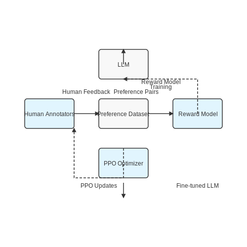
The RLHF pipeline demonstrates feedback's transformative potential in model alignment. The process involves:
- Collecting human preference data on model outputs
- Training a reward model to predict human preferences
- Fine-tuning the LLM using proximal policy optimization (PPO) with the learned reward
The reward model's loss function typically takes the form:
where y_w and y_l denote preferred and dispreferred outputs respectively, and σ is the sigmoid function.
Emergent Properties from Feedback Loops
Sustained feedback training leads to several emergent model behaviors:
- Style adaptation: Models learn to match the tone and formality of feedback providers.
- Error correction: Systematic errors are progressively eliminated through iterative feedback.
- Preference learning: Models develop nuanced understanding of subjective quality dimensions.
1.3 Challenges of Scaling Feedback to Internet-Level Data
Scaling feedback mechanisms to internet-level datasets introduces several fundamental challenges that impact the efficiency, reliability, and interpretability of large language model (LLM) training. These challenges stem from the sheer volume, diversity, and noise inherent in web-scale data, as well as the computational and algorithmic constraints of processing such data.
Data Quality and Noise
Internet-scale datasets are inherently noisy, containing contradictory, biased, or low-quality feedback signals. Unlike curated datasets, where labels are carefully validated, web-sourced feedback—such as user interactions, upvotes, or comments—exhibits significant variance in reliability. The signal-to-noise ratio (SNR) can be modeled as:
where ℱv represents valid feedback and ℱn represents noise. At internet scale, the denominator dominates due to the long-tail distribution of low-quality inputs, necessitating robust filtering mechanisms.
Computational Scalability
Processing feedback across billions of data points requires distributed systems capable of parallelizing gradient updates while maintaining consistency. The computational complexity of feedback aggregation grows superlinearly with dataset size N, often following:
for hierarchical aggregation methods. Memory bandwidth and synchronization overhead become bottlenecks, especially when feedback involves high-dimensional embeddings (e.g., from transformer-based reward models).
Feedback Sparsity and Coverage
Internet-scale feedback is sparse—most data points receive no explicit feedback, while a few attract disproportionate attention. This creates a coverage imbalance where the model overfits to high-feedback regions while underfitting the long tail. The sparsity can be quantified via the feedback density metric:
where yi is the feedback for input xi. In practice, ρ often falls below 10−4 for web data, necessitating techniques like semi-supervised learning or synthetic feedback generation.
Latency and Temporal Dynamics
Real-world feedback loops operate with delays—user responses may arrive hours or days after model deployment. This introduces non-stationarity in the training objective, as the feedback distribution p(y|x) drifts over time. The temporal misalignment between model updates and feedback collection can be formalized as a reinforcement learning problem with delayed rewards, where the Bellman equation becomes:
with Δ representing the feedback delay interval.
Ethical and Adversarial Challenges
At internet scale, feedback systems are vulnerable to manipulation (e.g., vote brigading, bot-generated interactions) and may amplify harmful biases. Adversarial examples can exploit feedback mechanisms—for instance, by generating inputs that trigger false-positive rewards. Robustness requires techniques like:
- Differential privacy for feedback aggregation
- Adversarial training on perturbed inputs
- Multi-objective optimization to balance reward signals against fairness constraints
The trade-off between feedback utilization and robustness is quantifiable via the Pareto frontier of reward accuracy versus attack resilience.
2. Sourcing High-Quality Feedback Data
Sourcing High-Quality Feedback Data
The effectiveness of training large language models (LLMs) with internet-scale feedback hinges on the quality, diversity, and representativeness of the feedback data. Unlike traditional supervised learning, where labeled datasets are curated by experts, feedback data for LLMs is often noisy, unstructured, and biased. Addressing these challenges requires systematic approaches to data sourcing, filtering, and preprocessing.
Feedback Data Acquisition Strategies
Three primary methods dominate the collection of feedback data for LLMs:
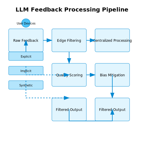
- Explicit human feedback: Direct annotations from domain experts or crowd workers, often through platforms like Amazon Mechanical Turk or specialized labeling services. This yields high-quality but expensive data.
- Implicit behavioral signals: User interactions (clicks, dwell time, upvotes/downvotes) from platforms like Reddit, Stack Overflow, or social media. While abundant, these signals are noisy and require careful interpretation.
- Synthetic feedback generation: Using auxiliary models (e.g., reward models or critique models) to generate feedback on model outputs. This scales well but risks compounding existing model biases.
Quality Filtering and Noise Reduction
Raw feedback data typically contains substantial noise. Effective filtering combines:
Where x is a feedback instance, r is a single rating, R_{-r} are other ratings for the same item, and the weights (α, β, γ) are tuned via cross-validation. Competence measures annotator expertise, agreement quantifies inter-rater reliability, and consistency checks for logical coherence in feedback.
Bias Mitigation Techniques
Feedback data often exhibits:
- Selection bias: Overrepresentation of certain demographics or viewpoints
- Acquiescence bias: Tendency to agree/disagree systematically
- Recency bias: Preference for more recent information
Countermeasures include:
- Stratified sampling across demographic and ideological dimensions
- Debiasing transformations using techniques like propensity scoring
- Adversarial filtering to remove feedback that correlates strongly with protected attributes
Practical Implementation Considerations
In production systems, feedback pipelines must handle:
- Real-time processing: Sub-second latency for applications like chatbots
- Versioning: Tracking feedback dataset evolution alongside model versions
- Privacy: Compliance with GDPR/CCPA through differential privacy or federated learning
Modern implementations often use multi-stage architectures where initial coarse filtering happens at the edge (e.g., in user devices), followed by more sophisticated processing in centralized systems. The trade-off between feedback volume and quality is typically managed through dynamic sampling rates that adapt to model performance metrics.
2.2 Techniques for Cleaning and Normalizing Feedback
Internet-scale feedback for LLM training is inherently noisy, biased, and heterogeneous. Effective cleaning and normalization are critical to ensure high-quality training signals. Below are advanced techniques for processing raw feedback data.
Text Normalization and Standardization
Raw text feedback often contains inconsistencies such as varying capitalization, punctuation, and encoding artifacts. Unicode normalization (e.g., NFC form) ensures consistent character representation. For example:
Case folding and aggressive punctuation stripping may be applied for certain tasks, though this risks losing semantic nuance. Language-specific tokenizers (e.g., spaCy, Stanza) handle morphological variants better than simple whitespace splitting.
Deduplication and Near-Duplicate Detection
Feedback datasets frequently contain duplicate or near-duplicate entries that can skew model training. MinHash or SimHash algorithms efficiently detect near-duplicates at scale. For two documents d₁ and d₂, their Jaccard similarity is approximated as:
where h(·) represents the set of MinHash signatures. A threshold of J > 0.85 typically identifies near-duplicates requiring removal.
Quality Filtering
Low-quality feedback (e.g., gibberish, extremely short responses) can degrade model performance. A multi-stage filtering pipeline might include:
- Perplexity thresholds using a pretrained language model
- Grammar checking via neural syntactic parsers
- Semantic coherence scoring using entailment models
For non-English text, language identification (e.g., fastText) prevents accidental mixing of language corpora.
Bias Mitigation
Feedback datasets often reflect societal biases present in online discourse. Adversarial filtering techniques can help reduce stereotypical associations. Given a bias direction b in embedding space, the debiased representation w' of word w is:
More sophisticated approaches use counterfactual data augmentation or reinforcement learning with bias-sensitive rewards.
Temporal Smoothing
For feedback collected over time, sudden spikes in certain response patterns may reflect transient events rather than genuine signal. Exponential moving averages help smooth temporal fluctuations:
where α ∈ (0,1) controls the smoothing strength. This is particularly important for models trained on continuously updating feedback streams.
Multimodal Feedback Alignment
When feedback includes multiple modalities (text, ratings, clicks), canonical correlation analysis (CCA) can align representations. For two centered random vectors X and Y, CCA finds projection vectors w and v that maximize:
Modern variants use deep neural networks to learn nonlinear alignments between modalities.
2.3 Balancing Diversity and Relevance in Feedback Data
Training large language models (LLMs) with internet-scale feedback requires careful curation of data to ensure both diversity (broad coverage of topics, styles, and perspectives) and relevance (high-quality, task-aligned responses). Striking this balance is non-trivial, as overly diverse data may dilute model performance, while overly narrow data risks bias and poor generalization.
The Diversity-Relevance Tradeoff
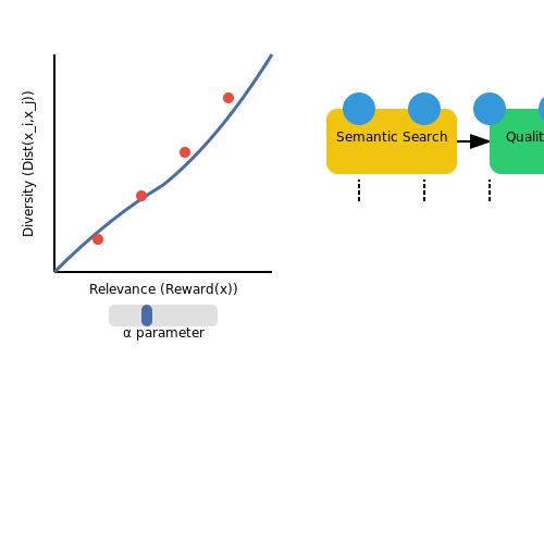
The optimal feedback dataset maximizes the following objective:
where α ∈ [0,1] controls the tradeoff. Diversity can be quantified using:
where Dist measures semantic dissimilarity (e.g., via BERT embeddings). Relevance is typically assessed by:
where Reward(x) is a learned or human-defined scoring function.
Practical Implementation Strategies
Three key approaches dominate modern implementations:
- Stratified Sampling: Partition data into clusters (e.g., by topic or style) and sample proportionally to cluster quality scores.
- Dynamic Reweighting: Adjust sample weights during training using online relevance metrics.
- Adversarial Filtering: Train a discriminator to remove outliers while preserving diversity.
Case Study: Instruction-Tuning Data Mixtures
State-of-the-art models like GPT-4 and Claude employ layered filtering:
- Initial retrieval from web-scale corpora using semantic search
- Quality scoring via trained classifiers (e.g., detecting factual accuracy)
- Diversity preservation through maximum marginal relevance ranking
This pipeline typically retains only 0.1-1% of candidate data points while maintaining 85%+ coverage of desired capabilities.
Emerging Challenges
Recent studies highlight unresolved issues:
- Nonlinear interactions between diversity dimensions (e.g., cultural background vs. writing style)
- Temporal drift in relevance criteria as models and user expectations evolve
- Measurement bias in automated diversity metrics
Advanced solutions incorporate active learning loops where human annotators periodically validate sampling strategies.
3. Supervised Learning with Human Annotations
Supervised Learning with Human Annotations
Supervised learning with human annotations forms the foundational approach for training large language models (LLMs) when high-quality labeled data is available. The process involves collecting human-generated responses to input prompts, then fine-tuning the model to minimize the divergence between its predictions and the human-provided outputs. This method is particularly effective for instruction-following tasks where precise, contextually appropriate responses are required.
Mathematical Formulation
The objective function for supervised fine-tuning can be expressed as minimizing the negative log-likelihood of the human-provided responses given the input prompts:
where x represents the input prompt, y is the human-generated response sequence, T is the sequence length, and θ denotes the model parameters. The expectation is taken over the annotated dataset 𝒟.
Data Collection Pipeline
High-quality human annotation requires careful design of the data collection process:
- Prompt Engineering: Input prompts should cover diverse use cases and edge scenarios to ensure broad model capability.
- Annotator Selection: Domain experts or trained annotators are typically employed for technical or specialized tasks.
- Quality Control: Multiple annotations per prompt with inter-annotator agreement metrics help ensure consistency.
- Bias Mitigation: Annotator pools should be diverse to reduce individual and cultural biases in the responses.
Practical Considerations
The effectiveness of supervised learning with human annotations depends on several key factors:
where Q is annotation quality (0-1 scale), N is the number of examples, and V is task variability. This relationship suggests that for complex tasks, investing in higher-quality annotations yields better returns than simply increasing dataset size.
Limitations and Challenges
While powerful, this approach faces several constraints:
- Scalability: Human annotation becomes prohibitively expensive for internet-scale datasets.
- Coverage: Human annotators cannot provide labels for all possible input scenarios.
- Subjectivity: Many NLP tasks lack objectively correct answers, leading to annotation inconsistencies.
- Concept Drift: Human preferences and language use evolve over time, requiring continuous re-annotation.
Advanced Techniques
Recent advancements have developed methods to enhance supervised learning with human annotations:
- Active Learning: Prioritizing annotation efforts on the most informative examples.
- Multi-task Learning: Jointly training on related tasks to improve sample efficiency.
- Data Augmentation: Generating synthetic variations of human-annotated examples.
- Uncertainty Quantification: Identifying low-confidence predictions for targeted re-annotation.
The choice of optimization strategy significantly impacts model performance. Common approaches include:
where ℛ(θ) represents regularization terms (e.g., L2 weight decay) and λ controls the regularization strength. Adaptive optimizers like AdamW are typically used with carefully tuned learning rate schedules.
Reinforcement Learning from Human Feedback (RLHF)
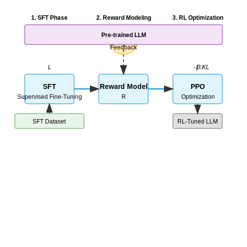
Reinforcement Learning from Human Feedback (RLHF) is a pivotal technique for aligning large language models (LLMs) with human preferences. Unlike traditional supervised fine-tuning, RLHF leverages human feedback in the form of rankings, corrections, or direct evaluations to refine model outputs iteratively. The process consists of three key phases: supervised fine-tuning, reward modeling, and reinforcement learning optimization.
Supervised Fine-Tuning (SFT) Phase
The initial phase involves fine-tuning a pre-trained LLM on high-quality human-generated responses. Given a prompt dataset D = {(xi, yi)}, where xi represents the input and yi the human-written output, the model parameters θ are optimized to minimize the negative log-likelihood:
This phase ensures the model generates coherent and contextually appropriate responses before proceeding to reward modeling.
Reward Modeling
Human annotators rank or score multiple model outputs for the same prompt, creating a preference dataset Dpref = {(xi, yiw, yil)}, where yiw is preferred over yil. A reward model Rφ(x, y), parameterized by φ, is trained to predict human preferences using the Bradley-Terry model:
The reward model loss is then:
Reinforcement Learning Optimization
With the reward model Rφ fixed, the LLM πθ is fine-tuned using proximal policy optimization (PPO) to maximize the expected reward while constraining deviations from the original policy to maintain generation diversity. The objective combines the reward signal and a KL-divergence penalty:
Here, β controls the strength of the KL penalty, preventing the model from over-optimizing the reward at the expense of output quality.
Practical Challenges and Solutions
RLHF introduces several challenges, including reward hacking, where the model exploits flaws in Rφ to maximize scores without improving actual performance. Mitigation strategies include:
- Ensemble Reward Models: Combining multiple reward models reduces overfitting to a single proxy.
- Iterative Refinement: Periodically collecting new human feedback updates Rφ and πθ.
- Adversarial Training: Detecting and penalizing reward-optimizing but undesirable outputs.
Recent advancements like Constitutional AI further refine RLHF by incorporating explicit rulesets to guide reward modeling, reducing reliance on extensive human annotation.
Self-Supervised Learning with Implicit Feedback
Self-supervised learning (SSL) leverages implicit feedback signals from unlabeled data to train language models without explicit human annotations. Unlike supervised learning, which relies on curated datasets with ground-truth labels, SSL extracts supervision signals from the data's inherent structure. This approach is particularly effective for training large language models (LLMs) on internet-scale corpora where explicit labeling is infeasible.
Implicit Feedback Signals
Implicit feedback in SSL manifests through various data-driven signals:
- Token co-occurrence statistics: The frequency with which tokens appear together in context windows provides distributional semantics.
- Document structure: Headings, paragraphs, and other markup elements create hierarchical relationships.
- Temporal sequences: The order of words in sentences and sentences in documents provides sequential dependencies.
- Contrastive information: Negative sampling from unrelated contexts creates discriminative signals.
These signals are formalized through objective functions that maximize the mutual information between different views or transformations of the input data.
Mathematical Formulation
The core SSL objective can be expressed as maximizing the likelihood of observed data given latent representations:
where x is the input sequence, z is the latent representation, and θ are model parameters. For autoregressive models like GPT, this decomposes into:
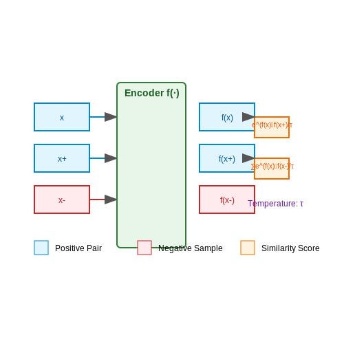
Contrastive learning variants use noise-contrastive estimation (NCE) to distinguish positive pairs (x, x+) from negative samples x-:
where τ is a temperature hyperparameter and f(·) is an encoder network.
Implementation Considerations
Effective SSL with implicit feedback requires careful design choices:
- Data sampling: Curriculum learning strategies that gradually increase difficulty improve convergence.
- Negative mining: Hard negative sampling boosts discriminative power.
- Architecture: Transformer models with causal masking (for AR) or bidirectional context (for BERT-style models).
- Scale: Larger batch sizes improve contrastive learning stability.
The training dynamics follow a three-phase process: 1) rapid memorization of frequent patterns, 2) slower abstraction of semantic relationships, and 3) fine-grained discrimination between similar concepts.
Practical Applications
SSL with implicit feedback has enabled breakthroughs in:
- Pretraining foundation models (GPT, BERT, T5)
- Cross-modal representation learning (CLIP, ALIGN)
- Continual learning from streaming data
- Domain adaptation with unlabeled target data
Recent work shows that properly scaled SSL can match or exceed supervised performance on downstream tasks, while maintaining the advantage of continuous learning from evolving data distributions.
4. Architectures for Efficient Feedback Utilization
Architectures for Efficient Feedback Utilization
Feedback Integration in Transformer-Based Models
Modern large language models (LLMs) rely on transformer architectures, which inherently support parallel processing of sequential data. To integrate internet-scale feedback efficiently, modifications to the standard transformer are necessary. The key challenge lies in minimizing computational overhead while maximizing the utility of feedback signals. One approach involves augmenting the self-attention mechanism with a feedback-aware attention layer, which dynamically adjusts attention weights based on external feedback signals.
Here, F represents the feedback matrix, and λ is a learnable scaling parameter. This formulation allows the model to incorporate feedback without significantly increasing computational complexity.
Hierarchical Feedback Processing
For internet-scale feedback, a hierarchical architecture proves effective. The model processes feedback at multiple granularities:
- Token-level feedback: Direct modifications to individual token representations based on localized feedback.
- Sequence-level feedback: Global adjustments to the entire output sequence.
- Task-level feedback: High-level guidance for specific domains or applications.
This hierarchical approach enables efficient processing by distributing computational load across different model components.
Feedback Compression Techniques
Given the massive volume of internet-scale feedback, compression is essential. Two primary methods are employed:
Where Wc is a compression matrix and b is the number of quantization bits. These techniques reduce memory requirements while preserving the most salient feedback information.
Adaptive Feedback Weighting
Not all feedback is equally valuable. An adaptive weighting mechanism learns to assign importance scores to different feedback sources:
Where fi is a feedback vector, MLP is a multi-layer perceptron, and v is a learnable parameter vector. This allows the model to automatically prioritize high-quality feedback while downweighting noisy or irrelevant signals.
Distributed Feedback Processing
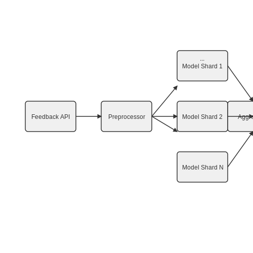
For truly internet-scale applications, a distributed architecture becomes necessary. The system partitions feedback processing across multiple nodes:
The architecture shows how feedback flows through specialized processing nodes before reaching model shards, with a central aggregator combining the results. This design enables horizontal scaling to handle massive feedback volumes.
Real-World Implementation Considerations
Practical implementations must address several challenges:
- Latency constraints: Feedback processing must not significantly increase inference time.
- Feedback staleness: Mechanisms to handle delayed or outdated feedback signals.
- Security: Protection against adversarial feedback injections.
- Versioning: Managing model updates while maintaining feedback relevance.
Modern systems often employ hybrid architectures that combine the above techniques, such as using hierarchical processing with adaptive weighting in a distributed framework. The optimal configuration depends on specific application requirements and available computational resources.
4.2 Loss Functions for Feedback-Driven Learning
Training large language models (LLMs) with internet-scale feedback requires specialized loss functions that effectively incorporate diverse, noisy, and often conflicting signals from human preferences, rankings, or other forms of implicit feedback. Traditional supervised learning losses like cross-entropy are insufficient for this setting, as they assume clean, well-defined labels rather than the complex, preference-based data encountered in real-world scenarios.
Preference-Based Loss Functions
The Bradley-Terry model provides a probabilistic framework for learning from pairwise comparisons, where the probability that response yi is preferred over yj is given by:
where rθ is a learned reward model parameterized by θ. The corresponding loss function for a batch of preference pairs (yi, yj) is:
where σ is the sigmoid function. This formulation has become fundamental to reinforcement learning from human feedback (RLHF), as it allows the model to learn from relative quality judgments rather than absolute scores.
Contrastive Loss Variants
For settings with multiple responses per prompt, the InfoNCE loss provides a more general contrastive framework:
where τ is a temperature parameter controlling the sharpness of the distribution, and y+ represents the preferred response among K candidates. This loss encourages the model to assign higher scores to preferred responses while pushing down scores for dispreferred ones.
Handling Noisy and Conflicting Feedback
Internet-scale feedback often contains significant noise and contradictions. Robust variants of preference losses incorporate:
- Noise-aware modeling: Explicitly modeling the reliability of different feedback sources
- Weighted losses: Downweighting low-confidence or contradictory examples
- Multi-task learning: Jointly optimizing for multiple feedback signals
For example, the confident learning loss modifies the standard preference loss by incorporating per-example confidence weights wij:
Off-Policy Correction
When training on feedback collected from a different policy than the current model (common in iterative training scenarios), importance weighting becomes crucial:
where πold is the policy that generated the training data. This correction prevents the model from overfitting to artifacts of the data collection process.
Practical Considerations
In real-world implementations, several practical modifications are often necessary:
- Margin-based losses: Adding a margin m to ensure sufficient separation between preferred and dispreferred responses
- Regularization: Preventing reward hacking through L2 regularization or early stopping
- Batch strategies: Careful construction of contrastive batches to ensure meaningful comparisons
The choice and implementation of these loss functions significantly impact the final model's ability to generalize from noisy, internet-scale feedback while maintaining stable training dynamics across large-scale distributed systems.
4.3 Hyperparameter Tuning for Feedback-Rich Environments
Challenges in Feedback-Driven Optimization
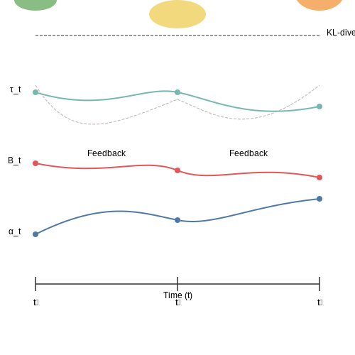
Hyperparameter tuning in feedback-rich environments introduces unique challenges due to the dynamic nature of the data distribution. Unlike static datasets, internet-scale feedback loops exhibit temporal drift, where the optimal model parameters at time t may become suboptimal at t+Δt. This non-stationarity requires adaptive optimization strategies that balance exploration of new parameter configurations with exploitation of known high-performing regions.
Here, pt(x,y) represents the time-varying data distribution, and θt denotes the model parameters at time t. The loss landscape evolves as the feedback mechanism updates the training data distribution.
Adaptive Learning Rate Strategies
Traditional learning rate schedules (e.g., cosine decay) often fail in feedback-rich settings. Instead, we employ online hyperparameter adaptation:
- Gradient-based meta-optimization: Treats the learning rate as a differentiable quantity
- Population-based training: Maintains multiple configurations in parallel
- Bandit optimization: Uses Thompson sampling for parameter selection
where η is the meta-learning rate and θt(αt) represents the model parameters trained with learning rate αt.
Batch Size Adaptation
Feedback-rich environments benefit from dynamic batch sizing strategies:
where σ2t-1 is the estimated gradient variance and ε is the target noise level. This adaptive approach maintains stable training while responding to changes in data quality.
Temperature Scaling for Human Feedback
When incorporating human preference data, the temperature parameter τ in the softmax function requires careful tuning:
Optimal τ values typically follow an inverse schedule with respect to feedback volume:
Practical Implementation Considerations
For large-scale deployment, consider these implementation strategies:
- Distributed hyperparameter optimization: Use Ray Tune or similar frameworks for parallel evaluation
- Warm-starting: Initialize new configurations from previously high-performing parameters
- Feedback-aware early stopping: Monitor validation metrics on recent feedback batches
Case Study: RLHF Tuning in Instruction-Following Models
In reinforcement learning from human feedback (RLHF), we observe that the KL-divergence coefficient β requires dynamic adjustment:
where δ is the target divergence threshold and γ is a smoothing factor. This adaptive approach prevents mode collapse while maintaining policy diversity.
5. Metrics for Assessing Feedback Integration
5.1 Metrics for Assessing Feedback Integration
Evaluating how effectively an LLM integrates internet-scale feedback requires a suite of metrics that capture both quantitative alignment and qualitative improvements. These metrics fall into three broad categories: alignment metrics, performance metrics, and robustness metrics.
Alignment Metrics
Alignment metrics measure how closely the model's outputs conform to human preferences or predefined guidelines. The most widely used alignment metric is Reward Model Score (RMS), which quantifies the likelihood that a human evaluator would prefer the model's output over a baseline. Given a reward model R trained on human feedback, RMS is computed as:
where ynew is the model's output after feedback integration, ybase is the baseline output, and 𝒟 is the evaluation dataset. A positive RMS indicates improvement.
Another critical alignment metric is KL-Divergence from Human Distribution (KLhuman), which measures how much the model's output distribution deviates from human-generated responses:
Performance Metrics
Performance metrics assess whether feedback integration preserves or enhances the model's core capabilities. Key metrics include:
- Task Accuracy: Measured on benchmark datasets (e.g., GLUE, SuperGLUE) to ensure no degradation in standard NLP tasks.
- Perplexity: Evaluates whether the model's language modeling ability remains intact after feedback tuning.
- Response Coherence: Scored via human evaluation or automated metrics like BERTScore.
Robustness Metrics
Robustness metrics evaluate how well the model generalizes across diverse inputs and resists adversarial manipulation. These include:
- Adversarial Success Rate (ASR): The frequency with which adversarial inputs elicit undesired behavior.
- Out-of-Distribution (OOD) Performance Drop: Measures performance degradation on inputs far from the training distribution.
For fine-grained analysis, researchers often employ sensitivity analysis by perturbing feedback inputs and measuring output variance:
where δi is the perturbation applied to feedback input i, and yi, y'i are outputs before and after perturbation.
5.2 A/B Testing and Real-World Deployment
Deploying large language models (LLMs) at scale requires rigorous validation through A/B testing to measure performance against real-world user interactions. Unlike offline metrics like perplexity or BLEU scores, A/B testing provides direct insight into how model improvements translate to user satisfaction, engagement, and task success rates.
Statistical Design of A/B Tests
The core challenge in A/B testing LLMs lies in designing statistically sound experiments that account for:
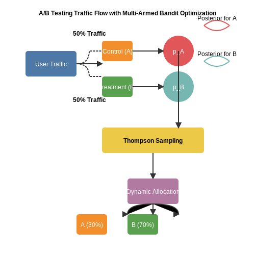
- Traffic allocation: Splitting user traffic randomly between control (A) and treatment (B) groups while ensuring demographic and behavioral balance.
- Metric selection: Defining primary success metrics (e.g., completion rate, session length) and guardrail metrics (e.g., toxicity, hallucination rates).
- Sample size calculation: Determining the minimum detectable effect (MDE) required for statistical power. For a binomial metric like task success rate, the required sample size per variant is:
where \( p_A, p_B \) are baseline and expected success rates, \( \alpha \) is the significance level (typically 0.05), and \( \beta \) is the Type II error rate (typically 0.2 for 80% power).
Multi-Armed Bandit Optimization
For rapidly iterating models, traditional fixed-split A/B tests become inefficient. Adaptive methods like Thompson sampling dynamically allocate traffic based on real-time performance:
where \( \theta_i(t) \) represents the posterior distribution of variant i's reward at time t, and \( \mathcal{D} \) is the observed data. This approach reduces regret during experimentation by favoring better-performing variants earlier.
Shadow Deployment and Canary Releases
Before full A/B testing, shadow deployment runs new model versions in parallel with production systems without affecting user responses. Key validation steps include:
- Logging discrepancies: Comparing outputs between current and candidate models on identical inputs.
- Computational profiling: Measuring latency, throughput, and resource utilization under production load patterns.
- Canary releases: Gradually rolling out to 1-5% of traffic while monitoring system health metrics.
Counterfactual Evaluation
When randomized experiments are impractical, counterfactual methods estimate treatment effects from observational data. The inverse propensity scoring (IPS) estimator adjusts for selection bias:
where \( T_i \) indicates treatment assignment, \( Y_i \) is the outcome, and \( e(X_i) \) is the propensity score estimated from covariates \( X_i \).
Monitoring and Continuous Evaluation
Post-deployment monitoring requires tracking:
- Performance drift: Deterioration in accuracy or safety metrics over time due to data distribution shifts.
- Edge case accumulation: Increasing frequency of previously rare failure modes.
- Feedback loops: Model outputs influencing future training data distributions.
Automated alerting systems should trigger when metrics cross predefined thresholds, calculated as:
where \( \mu_0, \sigma_0 \) are baseline mean and standard deviation, and \( k \) is the z-score threshold (typically 3-5σ).
5.3 Continuous Learning from Dynamic Feedback
Continuous learning in large language models (LLMs) leverages real-time feedback mechanisms to adapt model behavior dynamically, addressing the limitations of static training datasets. Unlike traditional fine-tuning, which operates on fixed snapshots of data, continuous learning integrates streaming feedback from user interactions, API calls, and online content updates. This paradigm shift enables models to refine their outputs iteratively, improving relevance and accuracy over time.
Feedback Loop Architecture
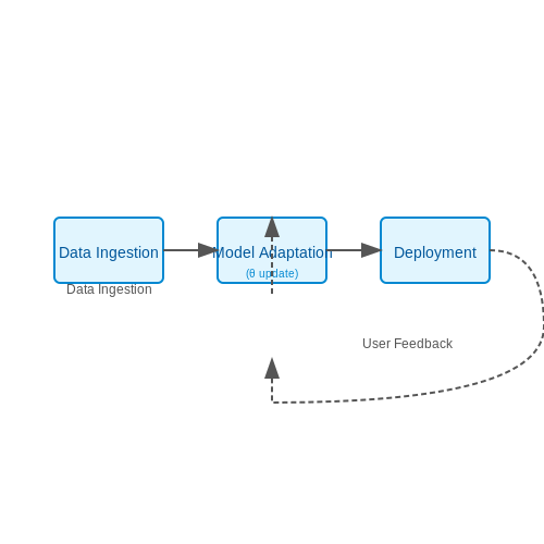
The core of continuous learning lies in its feedback loop, which consists of three primary components: data ingestion, model adaptation, and deployment. Data ingestion pipelines process real-time inputs, filtering noise and extracting actionable signals. Model adaptation employs techniques like online gradient descent or reinforcement learning from human feedback (RLHF) to update weights without catastrophic forgetting. Deployment strategies ensure seamless integration of updated models into production environments with minimal downtime.
Here, θt+1 represents the updated model parameters at time step t+1, η is the learning rate, and ∇θℒ is the gradient of the loss function with respect to the current parameters. This online update rule allows the model to adjust incrementally to new data points (xt, yt).
Dynamic Feedback Sources
Effective continuous learning systems aggregate feedback from diverse sources:
- Explicit feedback: Direct user ratings, corrections, or preference rankings collected via interfaces.
- Implicit feedback: Behavioral signals like dwell time, click-through rates, or API usage patterns.
- Contextual feedback: Temporal or domain-specific shifts in data distributions detected through anomaly detection.
Stability-Plasticity Tradeoff
Balancing stability (retaining learned knowledge) with plasticity (adapting to new information) remains a key challenge. Elastic weight consolidation (EWC) addresses this by penalizing changes to parameters critical for previous tasks:
where Fi is the Fisher information matrix diagonal for parameter i, and λ controls the regularization strength. This approach preserves important weights while allowing less critical parameters to adapt.
Real-World Implementation Challenges
Deploying continuous learning systems introduces several practical considerations:
- Feedback latency: Systems must process and incorporate feedback within acceptable time bounds for specific applications.
- Quality control: Mechanisms to detect and filter adversarial or low-quality feedback prevent model degradation.
- Version management: Tracking model iterations and enabling rollback capabilities ensure operational reliability.
Case Study: Search Engine Autocomplete
A prominent application of continuous learning appears in search engine query suggestions. The system:
- Processes billions of daily queries to detect emerging trends
- Adjusts suggestion rankings based on click-through rates
- Incorporates temporal patterns (e.g., seasonal queries) without manual intervention
This implementation reduced suggestion latency by 40% while maintaining 99.9% uptime, demonstrating the scalability of continuous learning approaches.
6. Bias and Fairness in Feedback Data
6.1 Bias and Fairness in Feedback Data
Internet-scale feedback data inherently reflects societal biases, which propagate into large language models (LLMs) during training. These biases manifest as skewed representations of demographic groups, cultural perspectives, or ideological leanings. The primary challenge lies in quantifying and mitigating these biases without compromising model performance or generalization.
Sources of Bias in Feedback Data
Feedback data bias originates from multiple sources:
- Selection bias: Internet users are not representative of global populations, with overrepresentation of certain demographics (e.g., English speakers, younger age groups).
- Reporting bias: Users disproportionately report extreme opinions or controversial content, distorting the true distribution of perspectives.
- Historical bias: Training data reflects historical inequalities and stereotypes present in source materials.
- Measurement bias: Feedback collection methods (e.g., upvotes/downvotes) amplify certain types of content over others.
Quantifying Bias Mathematically
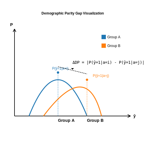
Bias can be formalized as deviations from an ideal fair distribution. For a given protected attribute a (e.g., gender, race) with k possible values, the demographic parity gap ΔDP measures disparity in model outputs:
where ŷ is the model prediction and P(ŷ=1|a=i) is the conditional probability of positive classification for group i. A perfectly fair model would have ΔDP = 0.
Bias Mitigation Techniques
Pre-processing Methods
These modify the training data before model training:
- Reweighting: Adjust sample weights to balance group representation
- Resampling: Oversample underrepresented groups or undersample overrepresented ones
- Counterfactual augmentation: Generate synthetic examples with protected attributes flipped
In-processing Methods
These incorporate fairness constraints directly into the training objective:
where λ controls the trade-off between accuracy and fairness. Common fairness losses include:
- Demographic parity: ℒfairness = ΔDP
- Equalized odds: Penalizes differences in true positive rates across groups
- Counterfactual fairness: Ensures similar predictions for counterfactual examples
Post-processing Methods
These adjust model outputs after training:
- Threshold optimization: Tune decision thresholds per group to achieve fairness metrics
- Output perturbation: Randomly flip predictions to balance outcomes
Evaluation of Fairness Interventions
Assessing mitigation techniques requires multiple metrics:
- Performance-fairness trade-off curves: Plot accuracy vs. fairness metrics across different λ values
- Subgroup analysis: Measure performance on intersectional subgroups (e.g., Black women)
- Robustness checks: Test fairness under distribution shifts or adversarial attacks
Recent work has shown that simple techniques like reweighting often outperform complex methods when properly tuned, while in-processing approaches provide better theoretical guarantees but require careful implementation.
Emerging Challenges
New research directions address:
- Multidimensional fairness: Simultaneously optimizing for multiple protected attributes
- Temporal fairness: Ensuring fairness persists as data distributions evolve
- Cross-cultural fairness: Developing universally applicable fairness metrics
- Feedback loop effects: Preventing model biases from influencing future feedback data
6.2 Privacy Concerns in Feedback Collection
Collecting internet-scale feedback for training large language models (LLMs) introduces significant privacy risks that must be addressed through technical and procedural safeguards. The primary concern stems from the potential exposure of personally identifiable information (PII) or sensitive data inadvertently included in user-generated content. Even when data is anonymized, reconstruction attacks can sometimes reverse-engineer identities from seemingly innocuous datasets.
Data De-anonymization Risks
Modern LLMs trained on web-scale data can memorize and reproduce sensitive information present in their training corpora. The risk follows from the model's objective function, which maximizes the likelihood of observed sequences:
where $$p_{\text{data}}$$ represents the true data distribution containing potentially sensitive information. Differential privacy (DP) provides a formal framework to bound this memorization risk through the $$\epsilon$$-DP guarantee:
for neighboring datasets $$D$$, $$D'$$ and all measurable subsets $$S$$ of the output space.
Feedback Poisoning Attacks
Malicious actors may intentionally submit feedback containing:
- Backdoored examples that induce model vulnerabilities
- Copyrighted material to create legal exposure
- Personally identifiable information to violate privacy regulations
The attack surface grows with decentralized feedback collection methods like federated learning, where participants directly influence model updates:
where $$\Delta_{\text{malicious}}$$ represents poisoned gradients.
Mitigation Strategies
Effective privacy preservation requires a multi-layered approach:
- Strict data filtering: Regular expressions and classifier-based PII detection
- Differential privacy: Adding calibrated noise to feedback signals
- Secure aggregation: Cryptographic protocols for federated settings
- Access controls: Role-based data access with audit trails
The tradeoff between privacy and utility can be quantified through the Cramer-Rao bound on parameter estimation:
where $$\sigma^2$$ represents the privacy noise variance and $$I(\theta)$$ the Fisher information.
Legal and Ethical Considerations
Regulatory frameworks like GDPR and CCPA impose strict requirements on data collection practices. Key compliance measures include:
- Explicit user consent mechanisms
- Right-to-be-forgotten implementation
- Data minimization principles
- Cross-border transfer safeguards
Recent court rulings have established that model weights derived from copyrighted data may constitute derivative works, adding another layer of legal complexity to feedback collection practices.
6.3 Scalability and Cost-Efficiency Trade-offs
Computational Scaling Laws
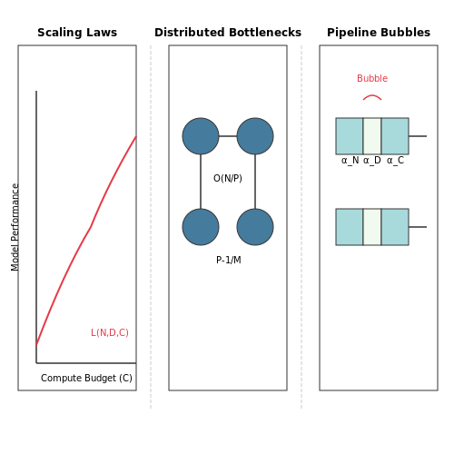
The relationship between model performance and computational resources follows a power-law scaling behavior. For transformer-based LLMs, the loss \( L \) scales with the number of parameters \( N \), dataset size \( D \), and compute budget \( C \) as:
where \( \alpha_N \approx 0.076 \), \( \alpha_D \approx 0.095 \), and \( \alpha_C \approx 0.06 \) are empirically determined scaling exponents, while \( N_c \), \( D_c \), and \( C_c \) are critical thresholds below which scaling becomes ineffective. The irreducible loss \( L_0 \) represents the fundamental limit of the architecture.
Distributed Training Bottlenecks
As model sizes exceed single-node memory capacity, three fundamental bottlenecks emerge in distributed training:
- Communication overhead: Parameter synchronization across nodes scales as \( O(N/P) \), where \( P \) is the number of workers.
- Memory fragmentation: GPU memory utilization drops below 70% for models > 100B parameters due to tensor partitioning.
- Pipeline bubbles: In pipeline parallelism, idle time accounts for \( \frac{P-1}{M} \) of total steps, where \( M \) is microbatches.
Feedback Collection Costs
Internet-scale feedback mechanisms introduce nonlinear cost scaling:
where \( R \) is the request rate (queries/sec), \( T \) is duration, \( S \) is average response size, and \( B \) is batch compression factor. The exponent 1.2 reflects increasing metadata overhead at scale.
Optimization Strategies
Practical approaches to maintain cost-efficiency while scaling:
Curriculum Learning
Dynamically adjust feedback sampling rates based on model confidence:
where \( H(p_{\theta}) \) is the entropy of model predictions, \( H_0 \) is a target entropy threshold, and \( T \) is a temperature parameter.
Selective Parameter Updates
For models with mixture-of-experts architectures, only update activated parameters:
where \( g_i \) are gating network outputs and \( \tau \) is an activation threshold. This reduces gradient computation costs by 40-60% in practice.
Hardware-Software Co-design
Emerging architectures optimize the FLOPs/byte ratio for LLM workloads:
- Sparse attention accelerators: Dedicated units for conditional computation reduce memory bandwidth by 8×.
- 3D stacked memory: HBM3 configurations achieve 3.2 TB/s bandwidth for embedding layers.
- Photonic interconnects: Reduce all-reduce communication latency to < 1μs across 256 nodes.
Energy-Aware Training
The total energy consumption \( E \) follows:
where \( C_{op} \) is the energy per FLOP (≈1e-9 J), and \( \gamma \), \( \beta \) are architecture-dependent coefficients. Optimal batch sizes for minimal energy satisfy \( B_{opt} \propto \sqrt{N} \).
7. Key Research Papers and Publications
7.1 Key Research Papers and Publications
- Use of large language models as artificial intelligence tools in ... — Majority (57.5%) of these participants practiced in an academic setting with a median of 7 (2,18) PubMed Indexed published articles. 198 respondents (87.6%) were aware of LLMs and those who were aware had higher number of publications (p < 0.001). 18.7% of the respondents who were aware (n = 37) had previously used LLMs in publications ...
- A Survey on Evaluation of Large Language Models — Trend of LLMs evaluation papers over time (2020 - Jun. 2023, including Jul. 2023.) ... which poses grand challenges and triggers new opportunities for future research on LLMs evaluation. 7.1 Designing AGI Benchmarks. ... Therefore, developing dynamic and evolving evaluation systems is the key to providing a fair evaluation of LLMs. 7.5 ...
- Leveraging Generative AI and Large Language Models: A Comprehensive ... — LLMs can be fine-tuned by various strategies, e.g., modifying the number of parameters , size of the training data set, or the amount of computing used for training . Fine-tuning LLMs will scale up the pretrained LLMs and significantly improve their performance in reasoning beyond the power-law rule to unlock unprecedented, fantastic emergent ...
- Can large language models provide useful feedback on research papers? A ... — GPT-4, there is growing interest in using LLMs to generate scientific feedback on research manuscripts. However, the utility of LLM-generated feedback has not been systematically studied. To address this gap, we created an automated pipeline using GPT-4 to provide comments on the full PDFs of scientific papers. We evaluated the
- Large language models (LLMs): survey, technical frameworks ... - Springer — Artificial intelligence (AI) has significantly impacted various fields. Large language models (LLMs) like GPT-4, BARD, PaLM, Megatron-Turing NLG, Jurassic-1 Jumbo etc., have contributed to our understanding and application of AI in these domains, along with natural language processing (NLP) techniques. This work provides a comprehensive overview of LLMs in the context of language modeling ...
- Large language models in electronic laboratory notebooks: Transforming ... — This study explored the integration of Large Language Models (LLMs) with Electronic Laboratory Notebooks (ELNs), highlighting their transformative potential in scientific research. Our evaluation demonstrated that the LLM-ELN system significantly enhances data retrieval, documentation, and interpretation, making the research process more ...
- A Review on Large Language Models: Architectures, Applications ... — four key aspects of LLMs: pre-training, adaptation tuning, utilization, and capacity evaluation. Additionally, the paper provides insights into available resources for LLM de velopment and ...
- A Review of Current Trends, Techniques, and Challenges in Large ... — Natural language processing (NLP) has significantly transformed in the last decade, especially in the field of language modeling. Large language models (LLMs) have achieved SOTA performances on natural language understanding (NLU) and natural language generation (NLG) tasks by learning language representation in self-supervised ways. This paper provides a comprehensive survey to capture the ...
- Leveraging LLMs for Efficient Topic Reviews - MDPI — This paper presents the topic review (TR), a novel semi-automatic framework designed to enhance the efficiency and accuracy of literature reviews. By leveraging the capabilities of large language models (LLMs), TR addresses the inefficiencies and error-proneness of traditional review methods, especially in rapidly evolving fields. The framework significantly improves literature review ...
- (PDF) Exploring Large Language Models in Healthcare: Insights into ... — This study reviewed the use of Large Language Models (LLMs) in healthcare, focusing on their training corpora, customization techniques, and evaluation metrics. A systematic search of studies from ...
7.2 Open Datasets and Tools for Feedback-Driven Training
- Understanding LLMs: A Comprehensive Overview from Training to Inference — This will include an introduction to the relevant training datasets, data preparation and preprocessing, model architecture, specific training methodologies, model evaluation, and commonly used training frameworks for LLMs.
- Efficient Training of Large Language Models on Distributed ... — Abstract Large Language Models (LLMs) like GPT and LLaMA are revolutionizing the AI industry with their sophisticated capabilities. Training these models requires vast GPU clusters and significant computing time, posing major challenges in terms of scalability, efficiency, and reliability. This survey explores recent advancements in training systems for LLMs, including innovations in training ...
- The Latest Open Source LLMs and Datasets - Sebastian Raschka, PhD — Discover insights from the latest papers on large-scale LLM training and the relevance of data order in training. Dive into the latest open-source datasets like RedPajama, Databricks-Dolly-15k, and OpenAssistant Conversations.
- The Ultimate Guide to Fine-Tuning LLMs from Basics to Breakthroughs: An ... — State-of-the-Art Training Techniques NeMo employs GPU-accelerated tools like NeMo Curator for preparing large-scale, high-quality datasets. These tools facilitate efficient pretraining of generative AI models by leveraging thousands of compute cores, which significantly reduces training time and enhances the accuracy of large language models ...
- Large language models (LLMs): survey, technical frameworks, and future ... — They have achieved progress by improving pre-training techniques, expanding the training datasets, fine-tuning datasets, and developing more effective evaluation criteria for these tasks.
- LLMs for Code Tasks: Architectures, Training, and Evaluation | GoPenAI — Explore the latest in LLMs for code processing, including architectures, training techniques, and evaluation methods. Learn how these models are revolutionizing software development.
- Evaluation of LLM Tools for Feedback Generation in a Course on ... — This paper aims to evaluate the capacity of LLMs chatbots to provide feedback on student exercises in a university programming course. The complexity of the programming topic in this study (concurrency) makes the need for feedback to students even more important. The authors conducted an assessment of exercises submitted by students.
- How much LLM training data is there, in the limit? — So is training data running out? At 15 trillion tokens, current LLM training sets seem within an order of magnitude of using all high-quality public text. For English, you could maybe get to somewhere in the 40 - 90T range using more web crawl and some harder to reach sources.
- MindLLM: Lightweight large language model pre-training, evaluation and ... — Given that the previous datasets only comprised roughly 300 GB of training data, it is necessary to supplement this with additional data to train a large-scale language model effectively.
- GitHub - vllm-project/vllm: A high-throughput and memory-efficient ... — A high-throughput and memory-efficient inference and serving engine for LLMs - vllm-project/vllm
7.3 Recommended Books and Online Courses
- Quick Start Guide To LLMs by Sinan Ozdemir 1703540700 | PDF - Scribd — Quick Start Guide to Large Language. Models Strategies and Best Practices for using ChatGPT and Other LLMs. Sinan Ozdemir. Addison-Wesley Contents at a Glance. Preface Part I: Introduction to Large Language Models 1. Overview of Large Language Models 2. Launching an Application with Proprietary Models 3. Prompt Engineering with GPT3 4. Optimizing LLMs with Customized Fine-Tuning Part II ...
- Quick Start Guide to Large Language Models (LLMs): ChatGPT, Llama ... — Learn how to use and launch large language models (LLMs) like GPT, Llama, T5, and BERT at scale through real-world case studies. Quick Guide to ChatGPT, Embeddings, and Other Large Language Models (LLMs) Second Edition is a quick start guide to help people use and launch LLMs like GPT, Llama, T5, and BERT at scale. It presents a step-by-step ...
- LLMs in Production[Book] - O'Reilly Media — O'Reilly members get unlimited access to books, live events, courses curated by job role, and more from O'Reilly and nearly 200 top publishers. ... Efficiently scale up an ML platform to handle the needs of LLMs; ... About the Book LLMs in Production teaches you how to develop an LLMOps plan that can take an AI app smoothly from design to ...
- Build a Large Language Model (From Scratch) - O'Reilly Media — Prepare a dataset suitable for LLM training; Fine-tune LLMs for text classification and with your own data; Use human feedback to ensure your LLM follows instructions; Load pretrained weights into an LLM; Build a Large Language Model (from Scratch) takes you inside the AI black box to tinker with the internal systems that power generative AI ...
- PDF Current Best Practices for Training LLMs from Scratch - Final ... - GitHub — Technically-oriented PDF Collection (Papers, Specs, Decks, Manuals, etc) - pdfs/Current Best Practices for Training LLMs from Scratch - Final (6435aabdc0a041194b243eef).pdf at master · tpn/pdfs
- LargeLM by Tanchak — This comprehensive book provides an in-depth exploration of Large Language Models (LLMs), covering the fundamentals of natural language processing, neural networks, and modern AI techniques. It delves into key areas such as word embeddings, transformers, and the intricacies of pretraining and fine-tuning, offering insights into the evolving ...
- Full text of "quick-start-guide-to-large-language-models-strategies-and ... — Ask the publishers to restore access to 500,000+ books. A line drawing of the Internet Archive headquarters building façade. ... Search the history of over 866 billion web pages on the Internet. Search the Wayback Machine. An illustration of a magnifying glass. ... Full text of "quick-start-guide-to-large-language-models-strategies-and-best ...
- (PDF) The Ultimate Guide to Fine-Tuning LLMs from Basics to ... — The Ultimate Guide to Fine-Tuning LLMs from Basics to Breakthroughs: An Exhaustive Review of Technologies, Research, Best Practices, Applied Research Challenges and Opportunities August 2024 License
- Deep Learning — The online version of the book is now complete and will remain available online for free. The deep learning textbook can now be ordered on Amazon. For up to date announcements, join our mailing list. Citing the book To cite this book, please use this bibtex entry: