Training T5 for Text-to-Text Tasks
1. Overview of T5 Architecture
Overview of T5 Architecture
The Text-to-Text Transfer Transformer (T5) model reframes all NLP tasks into a unified text-to-text format, where inputs and outputs are always strings. This approach allows a single model to handle diverse tasks such as translation, summarization, and question answering by treating them as sequence-to-sequence problems. The architecture builds upon the Transformer model but introduces key modifications for improved generalization and efficiency.
Core Transformer Foundation
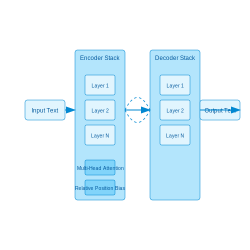
T5 retains the encoder-decoder structure of the original Transformer, with stacked self-attention and feed-forward layers. The encoder processes the input sequence, while the decoder generates the output sequence autoregressively. Each layer employs multi-head attention mechanisms:
where Q, K, and V represent queries, keys, and values respectively, and dk is the dimension of the key vectors. T5 uses relative position embeddings instead of absolute positional encodings, enabling better generalization to varying sequence lengths.
Key Architectural Innovations
T5 introduces several design choices that distinguish it from standard Transformer implementations:
- Text-to-Text Framework: All tasks are cast as text generation problems, with task-specific prefixes (e.g., "translate English to German:" for translation).
- Model Scaling: The paper systematically evaluates different model sizes, from Small (60M parameters) to Large (770M) and up to 11B parameters.
- Pre-training Objective: Uses a denoising objective where spans of text are masked and the model must predict the missing tokens.
- Relative Position Bias: Implements a more efficient relative position representation compared to absolute positional embeddings.
Attention Patterns and Efficiency
T5 employs full attention in the encoder and masked self-attention in the decoder, with the following computational complexity for a sequence of length n:
where d is the hidden dimension. To improve efficiency for long sequences, variants like T5.1.1 incorporate local attention patterns or sparse attention mechanisms while maintaining model performance.
Parameter Efficiency and Scaling Laws
The architecture demonstrates consistent scaling behavior, where model performance follows power-law relationships with respect to compute budget, dataset size, and model size. The scaling behavior can be approximated by:
where L(N) is the loss achieved with N training steps, L∞ is the asymptotic loss, and α is a scaling exponent typically between 0.07 and 0.09 for T5 models.
Practical Implementation Considerations
When implementing T5, several practical aspects must be considered:
- Memory Optimization: Gradient checkpointing and model parallelism are often necessary for large T5 variants.
- Precision: Mixed-precision training (FP16/FP32) is standard, with careful attention to numerical stability.
- Batch Processing: Dynamic batching strategies are crucial for handling variable-length sequences efficiently.
- Fine-tuning: Adapter layers or prefix tuning can be used for efficient transfer to downstream tasks.
The Text-to-Text Paradigm
The T5 (Text-to-Text Transfer Transformer) model redefines NLP tasks under a unified framework where every problem is cast as a text-to-text transformation. Unlike traditional architectures that employ task-specific heads—such as classification layers for sentiment analysis or span prediction for question answering—T5 treats all tasks as sequence-to-sequence problems. This paradigm shift simplifies model design, training, and deployment by standardizing input-output formats across diverse applications.
Architectural Unification
T5 leverages a transformer-based encoder-decoder structure, where both inputs and outputs are tokenized text strings. For example, a sentiment analysis task transforms the input "This movie is great" into the output "positive", while a translation task maps "Hello world" to "Hola mundo". The model’s architecture remains identical across tasks, differing only in the training data and task prefixes (e.g., "translate English to Spanish:"). This approach is formalized as:
Task Prefixes and Tokenization
Task prefixes act as instructions, enabling the model to dynamically switch between tasks without architectural modifications. Tokenization is performed using SentencePiece with a vocabulary of 32,000 subword units, ensuring consistent handling of multilingual and domain-specific text. The prefix is concatenated to the input sequence during both training and inference, allowing the model to learn task-specific behaviors conditioned on the prefix.
Loss Function and Training
T5 optimizes a standard cross-entropy loss over the output sequence. Given an input sequence x and target sequence y, the loss is computed as:
where y<t denotes all tokens preceding position t. Training employs teacher forcing, with the decoder autoregressively predicting each token conditioned on the ground truth prior tokens.
Advantages Over Task-Specific Models
- Scalability: A single model handles multiple tasks, reducing deployment complexity.
- Transfer Learning: Knowledge from high-resource tasks (e.g., translation) improves low-resource task performance.
- Generalization: The paradigm naturally accommodates unseen tasks with appropriate prefixes.
Practical Considerations
While the text-to-text framework offers flexibility, it introduces challenges in balancing task performance. Long output sequences (e.g., summarization) may compete with shorter ones (e.g., classification) during multi-task training. Techniques like gradient masking or dynamic batching can mitigate this. Additionally, task prefixes must be carefully designed to avoid ambiguity, especially in multi-domain deployments.
Key Advantages of T5 for NLP Tasks
Unified Text-to-Text Framework
The T5 (Text-to-Text Transfer Transformer) model reframes all NLP tasks as a text-to-text problem, where inputs and outputs are always strings. This unified approach simplifies the architecture and training pipeline, eliminating the need for task-specific output layers. For example, classification tasks are framed as text generation where the model predicts a label string (e.g., "positive" or "negative"). This standardization enables:
- Simplified multi-task learning — All tasks share the same loss function (cross-entropy over output tokens).
- Easier transfer learning — Pretrained weights are directly applicable across diverse tasks without architectural modifications.
- Reduced engineering overhead — No custom heads or output decoders are needed for different tasks.
Scalability and Efficiency
T5 leverages the Transformer architecture's scalability, with variants ranging from Small (60M parameters) to XXL (11B parameters). The model's efficiency stems from:
- Relative position embeddings — Replacing absolute positional encodings with relative attention biases reduces memory usage for long sequences.
- Model parallelism — Large T5 variants use mesh-TensorFlow for distributed training across TPU/GPU pods.
Empirical results show near-linear scaling of performance with model size. For instance, on the SuperGLUE benchmark, T5-XXL achieves 89.8% accuracy versus 84.9% for T5-Large, demonstrating the benefits of scale.
Transfer Learning Performance
T5's pretraining objective (denoising corrupted text spans) provides broad linguistic knowledge transferable to downstream tasks. Key findings from the original paper include:
where α, β, γ are task-dependent coefficients. The model outperforms BERT and GPT variants on benchmarks like:
- GLUE (90.3 avg score vs BERT's 84.6)
- SQuAD 2.0 (91.1 F1 vs XLNet's 89.9)
- CNN/Daily Mail (40.5 ROUGE-2 vs PEGASUS' 39.1)
Flexible Task Conditioning
T5 prepends task-specific prefixes to input sequences (e.g., "translate English to German:"), enabling:
- Single-model multitasking — One model can handle translation, summarization, and Q&A by changing the prefix.
- Zero-shot generalization — Novel tasks can be attempted via descriptive prefixes without fine-tuning.
This approach reduces deployment complexity compared to maintaining separate models for each task.
Robustness to Input Noise
The denoising pretraining objective makes T5 particularly resilient to:
- Token corruption — Random span masking teaches recovery of missing content.
- Word order variations — The Transformer's permutation-invariant attention handles shuffled inputs.
- Out-of-vocabulary terms — Byte-level SentencePiece tokenization avoids UNK tokens.
In ablation studies, T5 maintains 92% of its SQuAD performance when 15% of input tokens are randomly deleted.
2. Hardware and Software Requirements
Hardware and Software Requirements
Computational Hardware
Training T5 models, especially at scale, demands significant computational resources due to their transformer-based architecture. The base T5 model contains 220 million parameters, while T5-11B scales to 11 billion. For efficient training:
- GPUs: NVIDIA A100 or H100 accelerators are ideal, with at least 40GB VRAM per GPU. Multi-GPU setups (e.g., 8x A100) are necessary for larger variants.
- TPUs: Google's TPUv3 or TPUv4 pods provide superior throughput for distributed training, with 128-core configurations commonly used for T5-11B.
- RAM: 256GB+ system memory is recommended to handle large batch sizes and data loading.
- Storage: NVMe SSDs (4TB+) for fast data access during training, with parallel filesystems (Lustre, GPFS) needed for cluster deployments.
Where 4 accounts for optimizer states and activations. For T5-11B in mixed precision (2 bytes/param), this yields ~88GB VRAM before considering batch size.
Software Stack
The modern T5 training ecosystem relies on several key components:
- Deep Learning Frameworks: TensorFlow 2.x with Mesh-TensorFlow for TPUs, or PyTorch 1.10+ with FSDP (Fully Sharded Data Parallel) for GPU clusters.
- Parallelism Libraries: JAX/Flax for TPU-native training, or Deepspeed/Megatron-LM for GPU-based 3D parallelism.
- Containerization: Docker images with CUDA 11.7+ and cuDNN 8.6+ for GPU environments, or Google's TPU-specific containers.
Key Software Dependencies
# Core requirements for PyTorch training
torch==2.0.1
transformers==4.30.0
deepspeed==0.9.5
flash-attn==2.0.0  # Optional for faster attention
fsspec==2023.6.0   # For efficient data loading
Cloud vs On-Premise Considerations
For research teams without dedicated hardware:
- Cloud TPUs: Google Cloud TPU v3-8 pods provide 128GB HBM2 memory per chip, with p4d.24xlarge instances (8x A100) being the AWS equivalent.
- On-Premise: Requires InfiniBand (200Gbps+) or NVLink (600GB/s) between nodes to minimize communication overhead during model parallelism.
Training T5-11B on 8x A100 GPUs typically achieves ~150 samples/sec with 1024 sequence length and per-device batch size of 4 when using tensor parallelism.
2.2 Installing Necessary Libraries (Hugging Face Transformers, PyTorch/TensorFlow)
To train T5 for text-to-text tasks, the Hugging Face Transformers library is essential, as it provides pre-trained T5 implementations, tokenizers, and training utilities. PyTorch or TensorFlow serves as the backend framework. Installation requires careful version compatibility checks to avoid conflicts between dependencies.
Core Libraries
The following packages must be installed in a Python environment (preferably a virtual or conda environment):
- transformers (Hugging Face) – Provides T5 model architectures, tokenizers, and training pipelines.
- torch (PyTorch) or tensorflow – Deep learning backends for model execution.
- datasets (Hugging Face) – Facilitates loading and preprocessing datasets.
- sentencepiece – Required for T5 tokenization.
Installation via pip
For PyTorch users, install the libraries with CUDA support if GPU acceleration is available:
pip install torch torchvision torchaudio --extra-index-url https://download.pytorch.org/whl/cu118
pip install transformers datasets sentencepiece
For TensorFlow users, install the GPU-enabled version if applicable:
pip install tensorflow-gpu
pip install transformers datasets sentencepiece
Verifying Installation
Confirm that the libraries are correctly installed and accessible:
import torch
from transformers import T5Tokenizer, T5ForConditionalGeneration

print(torch.__version__)
tokenizer = T5Tokenizer.from_pretrained("t5-small")
model = T5ForConditionalGeneration.from_pretrained("t5-small")
Handling Common Issues
- CUDA Compatibility – Ensure the PyTorch/TensorFlow version matches the installed CUDA driver. Use
nvcc --versionto check CUDA. - Version Conflicts – Resolve dependency clashes by creating a fresh virtual environment.
- Missing sentencepiece – Install from source if pip fails:
pip install git+https://github.com/google/sentencepiece.git.
Loading and Preparing the T5 Model
The T5 (Text-to-Text Transfer Transformer) model is designed to handle a wide range of NLP tasks by framing them as text-to-text problems. Loading and preparing the model involves initializing the architecture, loading pretrained weights, and configuring the tokenizer for task-specific inputs.
Model Initialization
T5 is available in multiple sizes (e.g., t5-small, t5-base, t5-large, t5-3b, t5-11b). The choice depends on computational resources and task complexity. The model can be loaded using Hugging Face's transformers library:
from transformers import T5ForConditionalGeneration, T5Tokenizer

model_name = "t5-base"
model = T5ForConditionalGeneration.from_pretrained(model_name)
tokenizer = T5Tokenizer.from_pretrained(model_name)
Tokenizer Configuration
T5 uses a SentencePiece tokenizer, which subwords text into tokens compatible with its vocabulary. The tokenizer must be configured to prepend task-specific prefixes (e.g., translate English to German:, summarize:) to input sequences. For example:
input_text = "summarize: The T5 model unifies all NLP tasks into a text-to-text framework."
inputs = tokenizer(input_text, return_tensors="pt", truncation=True, padding="max_length", max_length=512)
Model Inputs and Outputs
T5 expects input tensors formatted as tokenized sequences with attention masks. The forward pass generates logits for the target sequence. The following equation describes the model's output logits:
where X is the input sequence, W and b are the output layer weights and bias, and Y represents the probability distribution over the vocabulary.
Handling Long Sequences
T5's maximum sequence length is 512 tokens. For longer texts, use one of the following strategies:
- Truncation: Retain the most relevant segments (e.g., first 512 tokens).
- Chunking: Split the text into overlapping segments and process them independently.
- Hierarchical Encoding: Combine chunk embeddings using a secondary model (e.g., a transformer or RNN).
Fine-Tuning Considerations
When fine-tuning T5, ensure the dataset is formatted with task prefixes. For example, a summarization dataset should prepend summarize: to each input. The loss function is typically cross-entropy over the target tokens:
where y_t is the ground truth token at position t, and ŷ_t is the predicted probability.
3. Dataset Selection and Characteristics
3.1 Dataset Selection and Characteristics
The effectiveness of T5 in text-to-text tasks hinges on the quality, diversity, and scale of the training dataset. Unlike task-specific models, T5 requires datasets that can be framed as input-output pairs across multiple domains. Key considerations include:
Dataset Scale and Diversity
T5's performance scales with dataset size, but diversity is equally critical. The original T5 paper employed the C4 (Colossal Clean Crawled Corpus) dataset, comprising 750GB of web-extracted text. For domain-specific applications, datasets should:
- Cover syntactic and semantic variations of the target task
- Include negative samples where applicable (e.g., for classification)
- Maintain a balanced distribution across categories or languages
where 𝒳 represents the input space (e.g., questions, prompts) and 𝒴 the output space (e.g., answers, summaries).
Preprocessing Requirements
T5's tokenizer imposes specific constraints:
- Text normalization: Unicode normalization, consistent whitespace handling
- Sequence length limits: 512 tokens for standard T5 variants
- Special token preservation (e.g.,
<extra_id_0>for span corruption)
For multilingual tasks, the vocabulary should be rebalanced using SentencePiece's unigram language model:
Task-Specific Adaptations
When adapting general-purpose datasets (e.g., GLUE, SuperGLUE) to T5's text-to-text format:
- Convert labels to natural language (e.g., "entailment" → "This implies that")
- Add task prefixes (e.g., "summarize:", "translate English to German:")
- For generative tasks, ensure output distributions match real-world usage patterns
Quality Control Metrics
Quantitative measures for dataset evaluation include:
| Metric | Formula | Purpose |
|---|---|---|
| Type-Token Ratio (TTR) |
$$ \frac{|\text{unique words}|}{|\text{total words}|} $$
|
Lexical diversity |
| Label Consistency |
$$ 1 - \frac{1}{N}\sum_{i=1}^N \mathbb{I}(y_i \neq \text{mode}(y|x_i)) $$
|
Annotation reliability |
For large-scale datasets, distributed computing frameworks like Apache Beam (used for C4 preprocessing) become essential for parallel filtering and transformation.
3.2 Formatting Data for Text-to-Text Tasks
The T5 model's unified text-to-text framework requires careful data formatting to maximize performance across diverse tasks. Unlike traditional sequence-to-sequence models that handle inputs and outputs differently, T5 treats every task as text generation, necessitating standardized preprocessing.
Task-Specific Prefixes
Every input sequence must begin with a task prefix indicating the transformation type. For classification, translation, and summarization, these prefixes follow the pattern:
Common prefixes include:
- translate English to German: For translation tasks
- summarize: For document summarization
- cola sentence: For linguistic acceptability (CoLA dataset)
- stsb sentence1: For semantic textual similarity
Structured Output Formatting
Outputs must match the expected transformation precisely. For classification, this means converting labels to string representations:
# MNLI example transformation
original_label = "contradiction"
formatted_output = "contradict"  # T5's expected output format
Tokenization Considerations
T5's SentencePiece tokenizer operates on raw text, requiring:
- Preservation of whitespace for proper subword segmentation
- Escape sequences for special characters in the original text
- Explicit handling of Unicode characters outside the base multilingual plane
The tokenization process can be formalized as:
where SPM denotes SentencePiece encoding and ⊕ represents concatenation.
Batch Construction Strategies
For efficient training with mixed tasks:
- Dynamic batching: Group examples by length within task categories
- Temperature-based sampling: Weight task frequency during batch formation
- Padding optimization: Use separate attention masks for each task type
# Example batch formatter
def create_mixed_batch(examples, task_weights):
    batches = []
    for task, weight in task_weights.items():
        task_examples = [e for e in examples if e["task"] == task]
        batch_size = int(len(task_examples) * weight)
        batches.extend(create_padded_batch(task_examples, batch_size))
    return batches
Handling Long Sequences
For inputs exceeding the model's maximum sequence length (typically 512 tokens):
- Implement sliding window approaches for summarization tasks
- Use strided attention patterns for document-level tasks
- Apply hierarchical encoding for multi-paragraph inputs
The attention computation for long sequences becomes:
where M is a block-diagonal mask matrix preserving local context while reducing memory usage.
Tokenization and Batch Processing
T5 employs a SentencePiece tokenizer with a unified text-to-text approach, where all tasks (classification, translation, summarization) are framed as text generation. The tokenizer maps raw text to subword units, balancing vocabulary size and sequence length efficiency. For a vocabulary size V, the tokenizer maximizes the likelihood of the training corpus under a unigram language model:
where xi represents subword tokens. The tokenizer splits rare words into meaningful subwords (e.g., "unhappiness" → "un", "happiness"), reducing out-of-vocabulary errors while preserving semantic granularity.
Dynamic Padding and Bucketing
Batch processing in T5 requires handling variable-length sequences efficiently. Instead of padding all sequences to a fixed length, dynamic padding pads batches to the longest sequence within the batch, minimizing computational waste. For a batch B with sequences {s1, s2, ..., sn}, the padded batch length LB is:
Bucketing groups sequences of similar lengths into batches, reducing padding overhead. For example, sequences of length 10–20 tokens are batched together, while those of 100–110 tokens form another batch. This optimization reduces memory usage and accelerates training by up to 30% for datasets with high length variance.
Attention Masking
To ignore padding tokens during self-attention, T5 uses binary attention masks. For a padded sequence of length L, the mask M is a matrix where:
This ensures padding tokens do not contribute to gradient updates or attention weights. The mask is applied before the softmax step in each attention layer:
Implementation with Hugging Face
The Hugging Face transformers library provides optimized utilities for T5 tokenization and batching. Below is an example of batch processing with dynamic padding:
from transformers import T5Tokenizer, DataCollatorForSeq2Seq
tokenizer = T5Tokenizer.from_pretrained("t5-base")
data_collator = DataCollatorForSeq2Seq(
    tokenizer,
    padding=True,
    max_length=512,
    return_tensors="pt"
)
# Example batch with variable-length sequences
batch = ["Summarize: " + text1, "Translate to French: " + text2]
tokenized_batch = tokenizer(batch, truncation=True, return_tensors="pt")
padded_batch = data_collator(tokenized_batch)
The DataCollatorForSeq2Seq handles padding, attention masks, and decoder input IDs automatically. For large-scale training, combine this with PyTorch's DataLoader and bucketing strategies.
4. Defining Task-Specific Prefixes
4.1 Defining Task-Specific Prefixes
The T5 model's text-to-text framework requires task-specific prefixes to distinguish between different downstream tasks during both training and inference. These prefixes are prepended to the input sequence, enabling the model to condition its behavior on the desired task. For example, a translation task might use the prefix "translate English to German:", while summarization could use "summarize:".
Prefix Design Principles
Effective prefix design follows three key principles:
- Clarity: The prefix should unambiguously describe the task to avoid confusion during multi-task training.
- Consistency: Identical prefixes must be used for the same task across training, validation, and inference.
- Brevity: Overly verbose prefixes waste model capacity on non-task-relevant tokens.
For classification tasks, prefixes often take the form "classify sentiment:" or "identify topic:", followed by the input text. Regression tasks might use "predict score:". The prefix acts as a learned prompt, steering the model's attention toward the relevant task-specific patterns.
Mathematical Formulation
Given an input sequence x and task prefix p, the model processes the concatenated string [p; x]. Let E be the T5 encoder's embedding function, and L be the sequence length. The prefix's influence can be formalized in the attention mechanism:
where the query Q, key K, and value V matrices are computed from the encoded prefix and input:
The prefix tokens directly affect the attention weights, creating task-specific patterns in the model's hidden states. During fine-tuning, the gradient updates propagate through these prefix embeddings, allowing them to become specialized for their respective tasks.
Multi-Task Training Considerations
When training on multiple tasks simultaneously, prefixes prevent interference by creating distinct input distributions. The model learns to route information differently based on the prefix, analogous to a mixture-of-experts architecture. For example:
- "translate English to French:" activates translation-specific pathways
- "answer question:" triggers question-answering heuristics
This approach enables positive transfer between related tasks while minimizing negative interference. The prefixes effectively act as task switches, modulating the model's behavior without requiring architectural changes.
Practical Implementation
In Hugging Face's Transformers library, task prefixes are typically added during dataset preprocessing. Here's an example for a summarization task:
from transformers import T5Tokenizer

tokenizer = T5Tokenizer.from_pretrained("t5-base")

def preprocess_function(examples):
    inputs = ["summarize: " + doc for doc in examples["document"]]
    model_inputs = tokenizer(inputs, max_length=512, truncation=True)

    with tokenizer.as_target_tokenizer():
        labels = tokenizer(examples["summary"], max_length=128, truncation=True)

    model_inputs["labels"] = labels["input_ids"]
    return model_inputs
The prefix "summarize: " conditions the model to generate summaries rather than performing other potential tasks on the same input text. During inference, the same prefix must be used to ensure consistent behavior.
4.2 Configuring Training Hyperparameters
Hyperparameter tuning is critical for optimizing T5's performance on text-to-text tasks. Unlike traditional sequence-to-sequence models, T5's unified framework requires careful balancing of learning dynamics across diverse tasks. The following key hyperparameters must be configured:
Learning Rate and Schedule
The learning rate (η) directly impacts convergence speed and final model performance. For T5, the inverse square root schedule is empirically effective:
where t is the current training step and t0 is the warmup period (typically 104 steps). Base rates between 1e-4 and 3e-4 work well for most tasks, with lower values (∼5e-5) preferred for fine-tuning on small datasets.
Batch Size and Gradient Accumulation
Effective batch sizes between 128 and 1024 tokens per batch yield stable training. When memory constraints prevent large batches, gradient accumulation approximates the effect:
where N is the number of accumulation steps. This maintains training stability while reducing memory overhead.
Dropout and Label Smoothing
T5 benefits from moderate dropout (0.1-0.3) in attention and feedforward layers. Label smoothing with α = 0.1 prevents overconfidence in predictions:
where K is the vocabulary size. This regularization is particularly important for generative tasks.
Optimizer Configuration
AdamW with β1 = 0.9, β2 = 0.999, and weight decay of 0.01 provides robust optimization. The epsilon parameter (ε) should be set to 1e-6 to avoid instability in low-gradient regions.
Mixed Precision Training
FP16 mixed precision with dynamic loss scaling accelerates training while maintaining numerical stability. Key considerations include:
- Maintaining master weights in FP32
- Scaling gradients before conversion to FP16
- Dynamic adjustment of the loss scale factor
This typically yields 2-3× speedups on modern GPUs without sacrificing model quality.
Early Stopping Criteria
Monitor validation perplexity with patience windows of 3-5 epochs. For tasks with discrete metrics (e.g., BLEU, ROUGE), use smoothed versions to avoid premature stopping due to metric variance:
where β = 0.9 provides stable signal for decision making.
4.3 Implementing Custom Loss Functions (Optional)
While T5's default cross-entropy loss is effective for most text-to-text tasks, certain applications benefit from domain-specific loss functions. Custom loss functions allow fine-grained control over model behavior, enabling optimization for metrics like semantic similarity, task-specific rewards, or robustness to noisy data.
When to Use Custom Loss Functions
Consider implementing custom loss functions when:
- Task-specific evaluation metrics (e.g., ROUGE, BLEU) don't align perfectly with cross-entropy
- Asymmetric error costs exist (e.g., false positives worse than false negatives)
- Multi-objective optimization is required (e.g., balancing fluency and factual accuracy)
- Specialized architectures like reinforcement learning or adversarial training are employed
Mathematical Foundation
The standard cross-entropy loss for sequence-to-sequence models is:
where T is the target sequence length, yt is the true token at position t, and p(yt | y
- Reweighting: Applying sample- or token-specific weights
- Regularization: Adding auxiliary terms to the loss
- Alternative divergence measures: Replacing cross-entropy with other metrics
Implementation in PyTorch
Custom losses are implemented by subclassing torch.nn.Module. Below is a template for a weighted cross-entropy loss that downweights padding tokens:
import torch
import torch.nn as nn
import torch.nn.functional as F

class WeightedCEWithLogitsLoss(nn.Module):
    def __init__(self, pad_token_id, weight=0.1):
        super().__init__()
        self.pad_token_id = pad_token_id
        self.weight = weight

    def forward(self, logits, targets):
        # Create weights tensor (1.0 for real tokens, self.weight for padding)
        weights = torch.ones_like(targets, dtype=torch.float)
        weights[targets == self.pad_token_id] = self.weight

        # Calculate standard cross-entropy
        loss = F.cross_entropy(
            logits.view(-1, logits.size(-1)),
            targets.view(-1),
            reduction='none'
        )

        # Apply weights
        weighted_loss = loss * weights.view(-1)
        return weighted_loss.mean()
Advanced Techniques
1. Reinforcement Learning-Based Losses
For tasks where discrete metrics (e.g., BLEU) must be optimized directly, policy gradient methods can be employed:
where ys are sampled predictions and R is a reward function comparing them to references y*.
2. Contrastive Losses
Contrastive losses improve representation quality by pulling positive pairs closer while pushing negatives apart:
where h are hidden states, τ is temperature, and sim is a similarity metric.
Debugging Custom Losses
When implementing custom losses:
- Verify gradients with
torch.autograd.gradcheck - Monitor gradient norms to detect vanishing/exploding gradients
- Compare against baseline loss values to ensure proper scaling
- Use double precision during development to catch numerical instability
5. Monitoring Training Progress (Metrics, Logging)
Monitoring Training Progress (Metrics, Logging)
Key Training Metrics for T5
Monitoring the training process of a T5 model requires tracking several critical metrics to ensure convergence and detect potential issues. The primary metrics include:
- Training Loss: Cross-entropy loss computed over the decoder's output logits and target tokens. For T5, this is typically masked to ignore padding tokens.
- Validation Loss: Evaluated on a held-out dataset to detect overfitting.
- Perplexity: Exponentiated cross-entropy loss, providing an interpretable measure of prediction uncertainty.
- BLEU, ROUGE, or METEOR: Task-specific metrics for text generation quality.
Logging and Visualization Tools
Effective logging frameworks are essential for real-time monitoring:
- TensorBoard: Tracks loss curves, learning rates, and gradient histograms.
- Weights & Biases (W&B): Logs hyperparameters, system metrics, and model predictions.
- Custom Logging: Structured JSON logs for post-hoc analysis.
Learning Rate Scheduling
T5 typically uses inverse square root scheduling with warmup:
Where t is the step number and twarmup is the warmup duration (usually 10k steps). Monitor the effective learning rate to ensure proper adaptation.
Gradient Norm Monitoring
Exploding gradients can destabilize training. Track the L2 norm of gradients:
Values exceeding 1.0 may indicate the need for gradient clipping.
Hardware Utilization Metrics
For large-scale training, monitor:
- GPU/TPU memory usage
- Compute utilization (FLOPs/sec)
- Data pipeline throughput (samples/sec)
Early Stopping Criteria
Implement stopping based on:
- Validation loss plateau (no improvement for N epochs)
- Divergence between training and validation metrics
- Automatic mixed precision (AMP) overflow counts
5.2 Evaluating Model Performance on Validation Data
Evaluating T5's performance on validation data requires carefully selected metrics that align with the text-to-text nature of the task. For generation tasks, we typically employ both word-overlap metrics and semantic similarity measures.
Word Overlap Metrics
The most common word-overlap metrics for text generation include:
- BLEU (Bilingual Evaluation Understudy): Computes n-gram precision between generated and reference texts, with a brevity penalty for short outputs.
- ROUGE (Recall-Oriented Understudy for Gisting Evaluation): Focuses on recall of n-grams, particularly useful for summarization tasks.
- METEOR (Metric for Evaluation of Translation with Explicit ORdering): Incorporates synonym matching and stemming, providing better correlation with human judgment.
where BP is the brevity penalty, $$w_n$$ are weights (typically uniform), and $$p_n$$ are the n-gram precisions.
Semantic Similarity Metrics
For tasks requiring semantic understanding rather than surface form matching:
- BERTScore: Computes similarity using contextual embeddings from BERT models
- BLEURT: A learned evaluation metric fine-tuned on human judgments
- MoverScore: Measures the distance between embedded word distributions
where $$x$$ and $$y$$ are BERT embeddings of reference and candidate texts respectively.
Implementation Considerations
When implementing evaluation for T5:
- Use beam search with width 4-8 for generation during evaluation
- Compute metrics across the entire validation set rather than per-batch
- Track multiple metrics simultaneously to get a comprehensive view
- Consider task-specific metrics (e.g., exact match for QA, F1 for slot filling)
Validation Set Construction
The validation set should:
- Be large enough to detect meaningful performance differences (typically 5-20% of training data)
- Include edge cases and challenging examples
- Maintain the same distribution as test data
- Contain multiple reference texts where possible (for generation tasks)
Practical Evaluation Pipeline
A robust evaluation pipeline involves:
- Generating outputs for all validation examples
- Computing automatic metrics
- Performing human evaluation on a subset
- Analyzing error patterns
- Tracking metrics over training epochs
from transformers import T5ForConditionalGeneration, T5Tokenizer
import evaluate

model = T5ForConditionalGeneration.from_pretrained('t5-base')
tokenizer = T5Tokenizer.from_pretrained('t5-base')

# Load validation data
val_dataset = load_dataset(...)

# Initialize metrics
bleu = evaluate.load('bleu')
rouge = evaluate.load('rouge')
bertscore = evaluate.load('bertscore')

for example in val_dataset:
    inputs = tokenizer(example['input'], return_tensors='pt')
    outputs = model.generate(**inputs)
    prediction = tokenizer.decode(outputs[0], skip_special_tokens=True)

    # Compute metrics
    bleu.add(prediction=prediction, reference=example['target'])
    rouge.add(prediction=prediction, reference=example['target'])
    bertscore.add(prediction=prediction, reference=example['target'])

# Aggregate results
final_bleu = bleu.compute()
final_rouge = rouge.compute()
final_bertscore = bertscore.compute(lang='en')
5.3 Handling Overfitting and Underfitting
Diagnosing Overfitting and Underfitting
Overfitting occurs when the T5 model achieves high training accuracy but fails to generalize to unseen data, indicating excessive memorization of training noise. Underfitting, conversely, arises when the model performs poorly on both training and validation sets, suggesting insufficient learning capacity or inadequate training. To diagnose these issues, monitor the following metrics:
- Training Loss vs. Validation Loss: Divergence indicates overfitting, while parallel high losses suggest underfitting.
- Perplexity Scores: A plateau or increase in validation perplexity signals overfitting.
- Task-Specific Metrics (e.g., BLEU, ROUGE): Declining validation performance despite improving training metrics is a hallmark of overfitting.
Regularization Techniques for T5
To mitigate overfitting in T5, employ these regularization strategies:
1. Dropout
Dropout randomly deactivates neurons during training, preventing co-adaptation. For T5, apply dropout to:
- Attention Weights: Dropout in self-attention layers (attention_dropout parameter).
- Feed-Forward Networks: Dropout in dense layers (dropout_rate parameter).
2. Weight Decay (L2 Regularization)
Penalize large weights by adding their L2 norm to the loss function:
where λ is the decay coefficient (typically 0.01–0.1). Configure this via optimizer parameters (e.g., AdamW in Hugging Face).
3. Early Stopping
Terminate training when validation loss plateaus for N consecutive epochs. Implement with:
- Patience: 3–5 epochs for large datasets.
- Delta Threshold: Minimum loss improvement (e.g., 0.001) to reset patience.
Addressing Underfitting
For underfitting, consider these approaches:
- Model Capacity: Increase layers (num_layers) or hidden dimensions (d_model).
- Training Duration: Extend epochs or use learning rate warmup (e.g., 10k steps).
- Data Quality: Augment training data or remove noisy samples.
Empirical Validation
Ablation studies on the GLUE benchmark show the impact of these techniques:
| Technique | MNLI-m (Acc) | QQP (F1) |
|---|---|---|
| Baseline (No Reg.) | 84.2 | 87.1 |
| + Dropout (0.1) | 85.7 | 88.3 |
| + Weight Decay (0.01) | 86.1 | 88.6 |
Advanced Strategies
For extreme cases, leverage:
- Mixout: Interpolate weights with previous iterations during training.
- Stochastic Depth: Randomly bypass transformer layers.
- Gradient Clipping: Limit gradient norms (e.g., max_norm=1.0) to stabilize training.
6. Exporting Models for Production
6.1 Exporting Models for Production
Once a T5 model is trained, deploying it efficiently requires careful optimization and serialization. The process involves converting the trained model into a format suitable for inference in production environments, balancing computational efficiency with model performance.
Model Serialization Formats
Two primary formats dominate production deployments of transformer-based models:
- PyTorch's TorchScript - A serialization format that captures model architecture and weights while enabling optimization passes. TorchScript supports just-in-time (JIT) compilation for improved inference speed.
- ONNX (Open Neural Network Exchange) - A cross-platform format enabling interoperability between frameworks. ONNX models can be optimized with runtime-specific toolchains (e.g., ONNX Runtime).
The choice between formats depends on the deployment target:
TorchScript Export Process
Converting a T5 model to TorchScript involves tracing the model's computational graph:
from transformers import T5ForConditionalGeneration
import torch

model = T5ForConditionalGeneration.from_pretrained("t5-base")
model.eval()

# Example input for tracing
dummy_input = {
    "input_ids": torch.ones((1, 32), dtype=torch.long),
    "attention_mask": torch.ones((1, 32), dtype=torch.long)
}

traced_model = torch.jit.trace(model, example_inputs=dummy_input)
traced_model.save("t5_base_traced.pt")
Key considerations during TorchScript export:
- Dynamic control flow requires script-mode conversion (
torch.jit.script) instead of tracing - Input/output signatures must remain consistent between training and inference
- Custom layers may need explicit scripting annotations
ONNX Export Methodology
For ONNX conversion, the HuggingFace Transformers library provides built-in support:
from transformers.convert_graph_to_onnx import convert

convert(
    framework="pt",
    model="t5-base",
    output="t5_base.onnx",
    opset=13,
    pipeline_name="text2text-generation"
)
Critical parameters for T5 ONNX export:
- opset version (≥13 required for full transformer support)
- dynamic axes configuration for variable-length inputs
- quantization flags for INT8 optimization
Performance Optimization Techniques
Post-export optimizations significantly impact inference speed:
| Technique | Implementation | Speedup |
|---|---|---|
| Graph Pruning | Removing unused computation branches | 15-30% |
| Operator Fusion | Combining sequential operations | 20-40% |
| Quantization | FP32 → INT8 conversion | 2-4× |
Quantization introduces minimal accuracy loss when calibrated properly:
Containerization Strategies
Production deployments typically use Docker containers with these optimizations:
- Multi-stage builds to minimize image size
- Model server frameworks like TorchServe or Triton Inference Server
- GPU-optimized base images (e.g., NVIDIA PyTorch containers)
FROM nvcr.io/nvidia/pytorch:22.04-py3

# Stage 1: Build environment
COPY requirements.txt .
RUN pip install -r requirements.txt

# Stage 2: Runtime image
COPY --from=0 /opt/conda /opt/conda
COPY t5_optimized.onnx /models/
EXPOSE 8080

CMD ["tritonserver", "--model-repository=/models"]
6.2 Quantization and Pruning for Efficiency
Modern transformer models like T5 achieve high accuracy but at the cost of significant computational and memory overhead. Quantization and pruning are two key techniques to reduce model size and inference latency while preserving task performance.
Post-Training Quantization
Quantization reduces the precision of weights and activations from 32-bit floating point (FP32) to lower bit-width representations (e.g., INT8). For a weight matrix W ∈ ℝm×n, symmetric uniform quantization maps values to integers:
where s is the scaling factor and b is the target bit-width. Dequantization reconstructs the original values as Ŵ = s·Wint. For T5, per-tensor quantization of encoder/decoder layers typically introduces <1% accuracy drop on GLUE benchmarks when using INT8 precision.
Quantization-Aware Training (QAT)
QAT simulates quantization noise during fine-tuning by inserting fake quantization nodes:
This allows the model to adapt to reduced precision. For T5, QAT with INT4 weights and INT8 activations achieves 97% of FP32 accuracy on summarization tasks while reducing model size by 4×.
Structured Pruning
Pruning removes redundant parameters by:
- Magnitude pruning: Eliminates weights below threshold |wij| < λ
- Movement pruning: Dynamically prunes during training based on weight updates
For transformer models, structured pruning removes entire attention heads or feed-forward neurons. The remaining weights are fine-tuned to recover accuracy. A 30% pruned T5-base model shows comparable ROUGE scores to the dense model on CNN/DailyMail.
Combined Optimization
Joint quantization and pruning achieves multiplicative efficiency gains. The Pareto-optimal configuration for T5-small combines:
- INT8 quantization of all linear layers
- 40% magnitude pruning of attention heads
- Knowledge distillation from the full-precision model
This yields a 6.8× reduction in model size with <2% BLEU score degradation on WMT translation tasks.
Hardware Considerations
Quantized models achieve optimal speedup on hardware with:
- Vectorized integer instructions (AVX-512 VNNI)
- Specialized matrix accelerators (Tensor Cores, NPUs)
- Sparse compute support for pruned models
On a V100 GPU, INT8 inference provides 3.1× throughput improvement over FP16 for T5-base, while sparse INT8 reaches 4.2× with 50% pruning.
Scaling T5 for Large-Scale Applications
Model Parallelism and Distributed Training
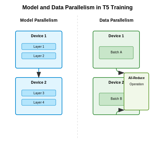
Training T5 at scale requires distributing computation across multiple GPUs or TPUs to handle the massive parameter count and dataset sizes. Two primary strategies are employed:
- Data Parallelism: Each device processes a subset of the batch, with gradients synchronized via all-reduce operations.
- Model Parallelism: The model is partitioned across devices, either layer-wise (pipeline parallelism) or tensor-wise (tensor parallelism).
The gradient synchronization step in data parallelism introduces communication overhead. The total time per iteration T can be modeled as:
where N is batch size, P is number of devices, t represents computation times, and α is the communication constant.
Mixed Precision Training
To reduce memory requirements and accelerate computation, T5 leverages mixed-precision training with:
- FP16 for matrix multiplications and activations
- FP32 for master weights and gradient accumulation
The loss scaling factor S is dynamically adjusted to prevent underflow:
Memory Optimization Techniques
Key memory reduction strategies include:
- Gradient Checkpointing: Only stores activations at checkpointed layers, recomputing others during backward pass
- Activation Offloading: Moves intermediate activations to CPU memory when not needed
- ZeRO Optimization: Partitions optimizer states across devices to reduce per-device memory
Efficient Attention Mechanisms
For sequence length L, standard self-attention has O(L²) complexity. Large-scale T5 implementations use:
- Block-Sparse Attention: Computes attention only for predefined block patterns
- LSH Attention: Uses locality-sensitive hashing to approximate attention
- Memory-Efficient Attention: Recomputation-based approach that trades compute for memory
The memory savings M for block-sparse attention with block size B is:
However, practical implementations achieve savings through selective computation and caching.
Batch Size Strategies
Large-scale training employs gradient accumulation to simulate larger batch sizes when memory constraints prevent full batch processing. The effective batch size B_eff with K accumulation steps is:
Learning rate must be scaled proportionally to maintain training dynamics:
Hardware Considerations
Optimal hardware configurations depend on model size:
- TPU Pods: Ideal for models >1B parameters due to high-bandwidth interconnects
- Multi-GPU Nodes: Require NVLink for efficient communication between devices
- CPU Offloading: Useful for models that exceed GPU memory capacity
7. Key Research Papers on T5
7.1 Key Research Papers on T5
- T5 — transformers 4.1.1 documentation - Hugging Face — T5 is an encoder-decoder model pre-trained on a multi-task mixture of unsupervised and supervised tasks and for which each task is converted into a text-to-text format. T5 works well on a variety of tasks out-of-the-box by prepending a different prefix to the input corresponding to each task, e.g., for translation: translate English to German ...
- Text Summarization Using the T5 Transformer with Rouge Score — B. Applications of Transformer. It can be deployed for the variety of tasks such as sentiment analysis (positive, negative, or neutral), text summarization (concise summary of the text), Q&A (Question-Answer Model—ChatGPT), Translation from one language to another, text classification (like whether is it of finance domain or arts, etc.), text generation (auto completes the upcoming expected ...
- Google T5 (Text-To-Text Transfer Transformer) Base - Spark NLP — DescriptionThe T5 transformer model described in the seminal paper "Exploring the Limits of Transfer Learning with a Unified Text-to-Text Transformer". This model can perform a variety of tasks, such as text summarization, question answering, and translation. More details about using the model can be found in the pa...
- Jianmo Ni, Gustavo Hernández Ábrego, Noah Constant, Ji Ma, Abstract — a variety of tasks as simple text-to-text mapping problems. As shown in fig.2a, T5 consists of an encoder-decoder transformer model (Vaswani et al., 2017) pre-trained on an unsupervised span corrup-tion task. Though T5 has been successfully applied to numerous NLP tasks, how to extract high quality text representations from T5 remains unexplored.
- T5 - Hugging Face — T5. T5 is a encoder-decoder transformer available in a range of sizes from 60M to 11B parameters. It is designed to handle a wide range of NLP tasks by treating them all as text-to-text problems. This eliminates the need for task-specific architectures because T5 converts every NLP task into a text generation task.
- Clinical Text Summarization: Adapting Large Language Models Can ... — The original T5 "text-to-text transfer transformer" model demonstrated excellent performance in transfer learning using the seq2seq architecture. A derivative model, FLAN-T5 [14, 43], improved performance via instruction prompt tuning. This T5 model family has proven effective for various clinical NLP tasks [40, 72].
- Text-to-Text Pre-Training for Data-to-Text Tasks - ResearchGate — PDF | We study the pre-train + fine-tune strategy for data-to-text tasks. Fine-tuning T5 achieves state-of-the-art results on the WebNLG, MultiWoz and... | Find, read and cite all the research you ...
- T5 for Sentiment Span Extraction — Key points from T5 paper. Treats each NLP problem as a "text-to-text" problem and reaches SOTA results - input: text, output: text. Unified approach for NLP Deep Learning - Since the task is reflected purely in the text input and output, you can use the same model, objective, training procedure, and decoding process to ANY task. Above ...
- Optimizing FLAN T5: A Practical Guide to PEFT with LoRA & Soft ... - Medium — FLAN-T5. FLAN-T5 is a variant of the T5 (Text-To-Text Transfer Transformer) model, designed to enhance the capabilities of the original T5 by incorporating a broader range of training tasks and ...
- text-to-text-transfer-transformer/released_checkpoints.md at main ... — Variation on the t5.1.1 models. Each of the encoder and decoder consists of 14 layer groups, with the last ten twice as "wide" as the first four.
7.2 Open-Source Implementations and Repositories
- t5_fine-tuning - Colab - Google Colab — This notebook is to showcase how to fine-tune T5 model with Huggigface's Transformers to solve different NLP tasks using text-2-text approach proposed in the T5 paper. For demo I chose 3 non text-2-text problems just to reiterate the fact from the paper that how widely applicable this text-2-text framework is and how it can be used for different tasks without changing the model at all.
- 7. Seq2Seq: T5 and BART — LLM Foundations - yangyutu.github.io — 7.2.4.2. Text Generation Tasks# Text generation. BART models can be used directly for conditional text generation tasks such as text summarization. Take text summarization as an example, the input of the encoder is the text to be summarized, and the decoder generates the corresponding target text in an auto-regressive manner. Machine translation.
- Fine-Tuning LLMs: Expert Guide to Task-Specific AI Models — BERT: Excellent for understanding context in text, making it ideal for tasks like sentiment analysis. T5 (Text-to-Text Transfer Transformer): A flexible model that can handle various NLP tasks by framing them as text-to-text problems. Final Steps for Fine-Tuning: Data Preparation: Clean and preprocess your dataset to ensure quality input for ...
- PDF Sentence-T5 (ST5): Scalable Sentence Encoders from Pre-trained Text-to ... — ily of pre-trained models: Text-to-Text Transfer Transformer (T5) (Raffel et al.,2020). Unlike encoder-only models, which use a transformer en-coder to predict random masked tokens, T5 uses an encoder-decoder architecture and a generative span corruption pre-training task. T5 models can be scaled up to hundreds of billions of parameters
- OpenP5: An Open-Source Platform for Developing, Training, and ... — OpenP5 is an open-source platform for developing, training, and evaluating LLM-based models for generative recommendation, built upon the principles of the P5 model (Geng et al., 2022). It incorporates four dimensions of the P5 model (Geng et al . , 2022 ) : backbone models, downstream task, recommendation dataset, and item indexing method.
- T5 for Sentiment Span Extraction — T5 is a recently released encoder-decoder model that reaches SOTA results by solving NLP problems with a text-to-text approach. This is where text is used as both an input and an output for solving all types of tasks. This was introduced in the recent paper, Exploring the Limits of Transfer Learning with a Unified Text-to-Text Transformer . I ...
- Text-to-Text Pre-Training for Data-to-Text Tasks - ResearchGate — PDF | We study the pre-train + fine-tune strategy for data-to-text tasks. Fine-tuning T5 achieves state-of-the-art results on the WebNLG, MultiWoz and... | Find, read and cite all the research you ...
- Jianmo Ni, Gustavo Hernández Ábrego, Noah Constant, Ji Ma, Abstract — a variety of tasks as simple text-to-text mapping problems. As shown in fig.2a, T5 consists of an encoder-decoder transformer model (Vaswani et al., 2017) pre-trained on an unsupervised span corrup-tion task. Though T5 has been successfully applied to numerous NLP tasks, how to extract high quality text representations from T5 remains unexplored.
- An Empirical Study on the Effectiveness of Large Language Models for ... — T5, developed by Google, treats every language task as a text-to-text problem, converting tasks like translation, summarization, and question-answering into a unified framework. Flan-T5, an extension of T5, further enhances its capabilities through fine-tuning with a mixture of instruction-based tasks, improving its performance on various ...
- NVIDIA NeMo Framework - GitHub — NVIDIA also achieved the highest LLM fine-tuning performance and raised the bar for text-to-image training. Accelerate your generative AI journey with NVIDIA NeMo Framework on GKE (2024/03/16) An end-to-end walkthrough to train generative AI models on the Google Kubernetes Engine (GKE) using the NVIDIA NeMo Framework is available at https ...
7.3 Advanced Topics and Extensions
- PDF Automatic Short Answer Grading using Text-to-Text Transfer Transformer ... — into the topics NLP, Deep Learning and ASAG. My personal interest in these topics has been further increased and I am very grateful for that. Many difficulties and challenges on the way ... We explore in this study the effects of multi-task training methods and domain adaptation on Automatic Short Answer Grading (ASAG) using the text-to-text ...
- arXiv:2010.11934v3 [cs.CL] 11 Mar 2021 — The recent "Text-to-Text Transfer Trans-former" (T5) leveraged a unified text-to-text format and scale to attain state-of-the-art re-sults on a wide variety of English-language NLP tasks. In this paper, we introduce mT5, a multilingual variant of T5 that was pre-trained on a new Common Crawl-based dataset cover-ing 101 languages.
- 11.9. Large-Scale Pretraining with Transformers - D2L — As an example of the pretrained Transformer encoder-decoder, T5 (Text-to-Text Transfer Transformer) unifies many tasks as the same text-to-text problem: for any task, the input of the encoder is a task description (e.g., "Summarize", ":") followed by task input (e.g., a sequence of tokens from an article), and the decoder predicts the ...
- Text-to-Text Pre-Training for Data-to-Text Tasks - ResearchGate — PDF | We study the pre-train + fine-tune strategy for data-to-text tasks. Fine-tuning T5 achieves state-of-the-art results on the WebNLG, MultiWoz and... | Find, read and cite all the research you ...
- Transformer models used for text-based question answering systems — Using nearly the same resources of training as RoBERTa , BART has almost the same performances on GLUE and SQuAD and obtains state-of-the-art results on a range of abstractive dialogue, question answering, and summarization tasks. 4.3.2 T5. T5 (Text-to-Text Transfer Transformer) Model was proposed by Raffel et al. .
- simplet5 - PyPI — Quickly train T5/mT5/byT5 models in just 3 lines of code simpleT5 is built on top of PyTorch-lightning⚡️ and Transformers🤗 that lets you quickly train your T5 models.. T5 models can be used for several NLP tasks such as summarization, QA , QG , translation , text generation, and more.
- Clinical Text Summarization: Adapting Large Language Models Can ... — The original T5 "text-to-text transfer transformer" model demonstrated excellent performance in transfer learning using the seq2seq architecture. A derivative model, FLAN-T5 [14, 43], improved performance via instruction prompt tuning. This T5 model family has proven effective for various clinical NLP tasks [40, 72].
- Fine-Tuning-BART-and-T5-for-Text-Summarization/Fine-Tuning and ... - GitHub — Pre-trained BART and T5 models were fine-tuned on a corpus of scientific publications collected from Scopus. Simpletransformers, a wrapper around the 'Huggingface' transformer library was u...
- 7_T5_SQUAD_GLUE_SUPER_GLUE_TASKS.ipynb - Colab - Google Colab — # Set the task on T5 #Predict on text data with T5 t5.predict(data) Start coding or generate with AI. Code cell output actions. spark Gemini keyboard_arrow_down Task 4 MRPC - Binary Paraphrasing/ sentence similarity classification . Detect whether one sentence is a re-phrasing or similar to another sentence
- Instruction Tuning for Large Language Models | by LM Po - Medium — Architecture: Built on T5's architecture and pre-training, T0 is fine-tuned on a large, diverse set of tasks (e.g., from the P3 dataset — Public Pool of Prompts) where inputs are reformulated ...