

Auction Price Prediction Using Historical Data
1. Key Factors Influencing Auction Prices
Key Factors Influencing Auction Prices
Market Demand and Supply Dynamics
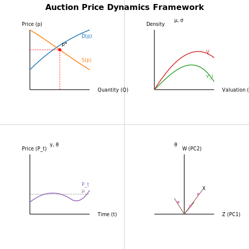
The equilibrium price in auctions emerges from the intersection of bidder demand and item supply. Let D(p) represent the demand function (number of bidders willing to pay price p) and S(p) the supply function (number of items available at price p). The clearing price p* satisfies:
In multi-unit auctions, this generalizes to vector-valued functions where D and S depend on the entire price schedule. The supply curve often exhibits discontinuities when lots contain unique items with no perfect substitutes.
Bidder Valuation Models
Advanced auction theory distinguishes three valuation frameworks:
- Private values: Each bidder knows their own valuation vi independently
- Common values: The item has an objective value V unknown to all bidders
- Affiliated values: Hybrid model where valuations correlate through shared signals
The winner's curse emerges prominently in common value auctions, where the winning bid tends to exceed the item's true value. Bayesian Nash equilibrium strategies account for this through shading:
where F is the valuation CDF and n the number of bidders.
Temporal Effects and Price Trajectories
Auction price series exhibit mean-reverting behavior with stochastic volatility. Let Pt be the price at time t, modeled by:
where θ is the mean reversion rate, μ the long-term mean, σ the volatility scale, and γ the elasticity parameter (typically 0.5-1.5). High-frequency auction data reveals microstructure effects where bid arrival times follow Hawkes processes:
Feature Engineering for Predictive Models
Effective price prediction requires constructing features that capture:
- Historical price momentum: EWMA of past closing prices with decay factor λ
- Bidder activity: Entropy of bid arrival times H = -Σpilog pi
- Market depth: Order book imbalance measured by (bids - asks)/(bids + asks)
- Seasonality: Fourier components for intraday/weekly patterns
The feature space X typically requires dimensionality reduction before model training. Principal Component Analysis (PCA) on normalized features yields:
where W contains the eigenvectors of XTX corresponding to the largest eigenvalues.
1.2 Types of Auction Data and Their Importance
Bid History and Temporal Dynamics
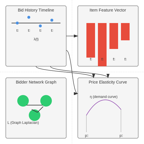
Auction bid histories capture the evolution of bids over time, forming a multivariate time series where each bid is a tuple (timestamp, bid_amount, bidder_id). The temporal spacing between bids encodes strategic behavior—early bids may signal low competition, while last-minute bidding (sniping) suggests high-value participants. Let the bid arrival process be modeled as a non-homogeneous Poisson process with intensity λ(t):
where T is auction end time, λ0 is baseline bid rate, and α, β govern late-bidding surge. The cumulative bid distribution F(b,t) reveals price formation mechanics.
Item Metadata and Feature Space
Beyond bids, auction items are characterized by high-dimensional feature vectors x ∈ ℝd spanning:
- Categorical: Product category, seller reputation tier, auction type (English/Dutch/Vickrey)
- Numerical: Reserve price, item age, shipping cost, historical sales percentiles
- Textual: Title/keyword embeddings from NLP models (e.g., BERT)
- Visual: Image features extracted via CNNs for condition assessment
Feature importance analysis using Shapley values or permutation tests identifies drivers like ∂P/∂(seller_rating) > 0 for luxury goods.
Bidder Network Graphs
Repeated interactions between bidders form a directed graph G=(V,E) where edge weights wij count how often bidder i outbids j. Spectral clustering reveals collusive rings—groups with abnormally high intra-cluster bidding density. The graph Laplacian L = D - A (degree matrix D, adjacency A) detects such anomalies when smallest eigenvalues deviate from random graph theory predictions.
Price Elasticity and Market Response
Historical auction archives allow estimating demand curves via censored regression. For n auctions with final prices pi and features xi, the Tobit model handles unsold items (prices below reserve):
Elasticity η = (∂Q/∂p)(p/Q) derived from such models informs optimal reserve pricing.
Cross-Auction Dependencies
Simultaneous auctions for substitutable goods exhibit game-theoretic interdependence. The revenue equivalence theorem breaks down when bidders face budget constraints across k parallel auctions. The allocation problem becomes a linear program where bidder j maximizes:
where xij ∈ {0,1} indicates winning, vij is private valuation, and Bj is total budget. Historical data reveals empirical violation rates of pure strategy Nash equilibria.
1.3 Challenges in Auction Price Prediction
Non-Stationary and Volatile Market Dynamics
Auction markets exhibit non-stationary behavior where statistical properties such as mean and variance change over time. This volatility arises from external shocks, macroeconomic trends, and shifts in buyer preferences. Traditional time-series models like ARIMA assume stationarity, requiring differencing or transformation:
where B is the backshift operator and d is the differencing order. However, excessive differencing may erase meaningful patterns, while insufficient differencing fails to address non-stationarity.
Sparse and Irregular Data Sampling
High-value auctions (e.g., art, real estate) occur infrequently, resulting in sparse temporal data. Unlike stock markets with tick-level data, auction events may have gaps spanning weeks or months. This irregularity complicates the application of sequential models like RNNs, which assume equidistant timesteps. Imputation strategies often introduce bias, while ignoring missing data reduces training samples.
Multimodal Price Distributions
Final hammer prices frequently follow multimodal distributions due to:
- Discrete valuation tiers: Buyers cluster around psychological price points (e.g., $10,000 thresholds)
- Market segmentation: Competing buyer groups (collectors vs. investors) with divergent valuation models
Gaussian-based regression underestimates tail risks in such distributions. Mixture density networks (MDNs) provide better modeling:
Exogenous Variable Integration
Macroeconomic indicators (interest rates, GDP growth) and asset-specific features (provenance, condition reports) influence prices but exhibit complex, non-linear interactions. Standard feature concatenation in neural networks often fails to capture hierarchical relationships. Attention mechanisms or graph neural networks can model these dependencies more effectively by learning conditional importance weights:
Strategic Bidder Behavior
Bidders employ complex strategies like bid shading or jump bidding that distort the apparent valuation landscape. Game-theoretic approaches partially model this through Bayesian Nash equilibrium concepts:
where β(vi) is the optimal bid for a player with valuation vi in an n-player first-price auction, and F is the cumulative distribution of valuations. However, real-world bidding often deviates from theoretical equilibria.
Concept Drift in Valuation Models
The mapping between item features and realized prices evolves due to changing tastes or new information. A painting's attribution reassessment or an athlete's career injury can abruptly alter market perception. Online learning techniques like dynamic Bayesian networks or continual learning architectures are necessary to adapt models without catastrophic forgetting of historical patterns.
2. Sources of Historical Auction Data
2.1 Sources of Historical Auction Data
Historical auction data is critical for training robust price prediction models, but sourcing high-quality datasets requires understanding the trade-offs between coverage, granularity, and accessibility. The most reliable sources fall into three categories: institutional auction houses, government repositories, and commercial data aggregators.
Institutional Auction House Archives
Major auction houses like Sotheby's, Christie's, and Phillips maintain extensive digital archives spanning decades. These datasets are particularly valuable because they include:
- High-resolution images and condition reports for each lot
- Detailed provenance records
- Bid-level transaction histories (hammer prices, buyer premiums)
- Expert-curated category metadata (e.g., "Post-War Contemporary Art")
However, access is often restricted through proprietary APIs with rate limits. The data structure typically follows a nested JSON format where each auction event contains multiple lots:
{
  "auction_id": "CH12345",
  "date": "2023-05-15",
  "location": "New York",
  "lots": [
    {
      "lot_number": 35,
      "artist": "Yayoi Kusama",
      "title": "Infinity Nets (TWHOQ)",
      "estimate_low": 800000,
      "estimate_high": 1200000,
      "hammer_price": 950000,
      "premium": 1140000,
      "currency": "USD"
    }
  ]
}
Government Cultural Heritage Databases
National archives and cultural ministries often publish auction records for regulatory compliance. For example:
- China's State Administration of Cultural Heritage maintains a complete database of all antiquities sold through licensed channels
- EU Member States report art market transactions under anti-money laundering directives (AMLD5)
These sources provide broad coverage but lack the item-level detail of auction house data. The temporal resolution is also coarser, typically aggregated quarterly or annually.
Commercial Data Aggregators
Third-party platforms like Artnet, MutualArt, and Pi-eX normalize auction data across multiple sources. Their value lies in:
- Cross-institutional price indices (e.g., Artnet Price Database covers 1,800+ auction houses)
- Inflation-adjusted time series going back to the 1980s
- Derived metrics like price-per-square-cm for visual arts
The data quality varies significantly by aggregator. Some key validation checks include:
For rare categories like vintage watches or classic cars, specialized aggregators like WatchCharts and Hagerty provide more granular data including movement serial numbers and vehicle identification numbers (VINs).
Web Scraping Challenges
When direct APIs are unavailable, researchers often resort to web scraping auction results. This introduces several technical considerations:
- Dynamic content rendering requires headless browsers (Puppeteer, Playwright)
- Anti-scraping measures like Cloudflare protection may necessitate proxy rotation
- Data normalization is complex due to inconsistent field naming across sources
The scraping process can be formalized as a Markov Decision Process where each state s represents a webpage and actions a are navigation choices:
Where R(s,a) is the immediate reward (data extracted) and γ discounts future rewards from deeper site traversal.
2.2 Data Cleaning and Handling Missing Values
Raw auction datasets often contain missing values, outliers, and inconsistencies that degrade model performance if unaddressed. Advanced techniques for imputation and anomaly detection are essential for robust price prediction.
Identifying Missing Data Patterns
Missing data falls into three categories defined by Rubin (1976):
- Missing Completely at Random (MCAR): No relationship between missingness and observed/unobserved data.
- Missing at Random (MAR): Missingness depends only on observed data.
- Missing Not at Random (MNAR): Missingness depends on unobserved data.
For auction data, test these mechanisms using Little's MCAR test:
where Oi and Ei are observed and expected missing value counts per feature.
Advanced Imputation Methods
1. Multivariate Imputation by Chained Equations (MICE)
MICE iteratively models each feature with missing values as a function of other features. For p features:
- Initialize missing values with mean/mode
- For iteration t = 1 to T:
$$ x_j^t = f_j(x_{-j}^{t-1}, heta_j^{t-1}) + \epsilon_j $$
- Update parameters θj via regression
2. Deep Learning Approaches
Generative Adversarial Imputation Networks (GAIN) outperform traditional methods for complex auction data distributions:
where G is the generator, D the discriminator, X the data matrix, and M the missingness mask.
Handling Auction-Specific Anomalies
Auction data often contains:
- Shill bidding patterns: Detect using exponentially weighted moving variance:
$$ \sigma_t^2 = \alpha (r_t - \mu_{t-1})^2 + (1-\alpha)\sigma_{t-1}^2 $$
- Outlier bids: Apply modified z-scores with median absolute deviation:
$$ M_i = \frac{0.6745(x_i - \tilde{x})}{\text{MAD}} $$
Implementation Considerations
For time-series auction data, combine imputation with temporal modeling:
import numpy as np
from sklearn.experimental import enable_iterative_imputer
from sklearn.impute import IterativeImputer

# Create MICE imputer with BayesianRidge estimator
imputer = IterativeImputer(
    estimator=BayesianRidge(),
    n_nearest_features=5,
    initial_strategy='median',
    max_iter=50,
    tol=1e-6
)

# Fit-transform on auction price matrix
clean_data = imputer.fit_transform(auction_data)
Key parameters to optimize include n_nearest_features (for high-dimensional data) and tol (convergence threshold).
2.3 Feature Engineering for Auction Data
Temporal Features
Auction dynamics are inherently time-dependent, making temporal features critical for price prediction. The most effective temporal features include:
- Time since auction start: The elapsed time normalized by the total auction duration, calculated as:
- Bid arrival intensity: The instantaneous rate of bids per unit time, computed using exponential smoothing:
where α is the smoothing factor (typically 0.1-0.3). This captures the momentum of bidding activity.
Bidder Behavior Features
Strategic bidder behavior can be quantified through several derived metrics:
- Bid aggressiveness: The relative jump between consecutive bids from the same bidder:
- Bid timing patterns: The distribution of inter-bid times for each bidder, modeled as a Weibull distribution:
where λ and k capture characteristic waiting times and consistency of bidding behavior.
Market Context Features
External market conditions significantly impact auction outcomes. Key features include:
- Competing auction density: The number of simultaneous auctions for similar items, weighted by geographic proximity:
where dij is the distance between auctions and sj is the similarity score.
- Price momentum: The moving average of closing price ratios for comparable items:
Feature Interactions
Non-linear interactions between features often contain predictive signals:
- Bidder concentration effect: The product of unique bidder count and average bid increment:
- Temporal bidding pressure: Interaction between time remaining and bid frequency:
Embedding-Based Features
For high-cardinality categorical variables like bidder IDs:
- Bidder embeddings: Learned low-dimensional representations from historical bidding patterns using neural networks:
where hi is the bidder's historical feature vector and fθ is a 2-layer MLP.
Feature Selection
Optimal feature subsets can be identified through:
- Shapley value analysis for non-linear model interpretability
- Mutual information scores for non-parametric dependence
- Recursive feature elimination with cross-validation
3. Visualizing Price Distributions and Trends
3.1 Visualizing Price Distributions and Trends
Kernel Density Estimation for Price Distributions
When analyzing auction price data, the underlying distribution often deviates from standard parametric forms. Kernel density estimation (KDE) provides a non-parametric approach to estimate the probability density function. Given a sample of prices {x1, x2, ..., xn}, the KDE f̂(x) is computed as:
where K is the kernel function (typically Gaussian) and h is the bandwidth controlling smoothness. The optimal bandwidth minimizes the mean integrated squared error (MISE):
For multi-modal distributions common in auction data, adaptive KDE methods that vary bandwidth locally often outperform fixed-bandwidth approaches.
Quantile-Quantile Plots for Normality Assessment
Q-Q plots compare sample quantiles against theoretical quantiles from a reference distribution (e.g., normal). Let F-1 be the quantile function of the reference distribution. For ordered price data x(1) ≤ ... ≤ x(n), the points are:
Deviations from linearity indicate non-normality - heavy tails manifest as curvature at the ends, while skewness appears as systematic asymmetry.
Time Series Decomposition
Auction prices often exhibit complex temporal patterns decomposable into:
- Trend (Tt): Long-term directional movement
- Seasonality (St): Regular periodic fluctuations
- Residuals (Rt): Irregular noise
The additive model is:
For multiplicative patterns (common when variance grows with price), a logarithmic transform converts the model to additive form. STL (Seasonal-Trend decomposition using Loess) provides robust estimation even with missing data.
Visualizing High-Dimensional Relationships
When prices depend on multiple features (e.g., item condition, auction duration), dimensionality reduction techniques reveal latent structure. t-SNE minimizes the Kullback-Leibler divergence between high-dimensional and low-dimensional probability distributions:
where pij and qij are pairwise similarities in original and embedded spaces. For large datasets, UMAP often provides better scalability while preserving global structure.
Interactive Visualization with Plotly
Static plots have limitations for exploring complex auction data. Plotly's JavaScript backend enables interactive features:
- Hover tooltips showing exact values
- Zooming into specific time periods
- Dynamic filtering by categorical variables
- Linked views across multiple plots
import plotly.express as px
fig = px.scatter(df, x='auction_duration', y='final_price',
                 color='item_condition', trendline='lowess',
                 title='Price vs Duration by Condition')
fig.update_layout(hovermode='x unified')
fig.show()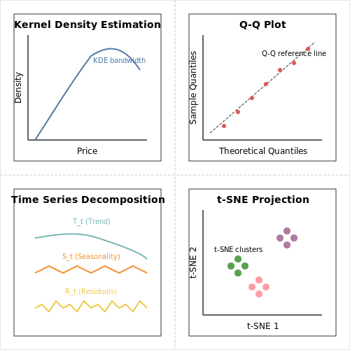
3.2 Correlation Analysis Between Features and Prices
Correlation analysis quantifies the linear relationship between auction features and final prices, providing insight into which variables most strongly influence outcomes. For auction price prediction, understanding these dependencies is critical for feature selection and model interpretability.
Pearson Correlation Coefficient
The Pearson correlation coefficient r measures linear dependence between two variables X (feature) and Y (price), ranging from -1 (perfect negative correlation) to +1 (perfect positive correlation). The population Pearson coefficient is derived as:
For a sample of n observations, the estimator becomes:
In auction datasets, common strongly correlated features include item rarity (Spearman ρ ≈ 0.6-0.8), historical sale frequency (r ≈ -0.4 to -0.7), and condition grades (r ≈ 0.5-0.9). Time-dependent features like auction duration often show nonlinear relationships better captured by rank correlation methods.
Partial Correlation
When features exhibit multicollinearity, partial correlation identifies the unique relationship between a feature and price while controlling for other variables. For features X, Y with confounding variable Z, the first-order partial correlation is:
This reveals whether a feature's apparent correlation with price is spurious or mediated by other factors. In art auctions, for example, artist name may show high raw correlation with price (r = 0.75), but partial correlation controlling for artwork size and medium may reduce this to r = 0.32, indicating substantial confounding.
Cross-Correlation for Time Series
For sequential auction data, cross-correlation functions (CCF) identify lagged relationships between price and temporal features:
where τ is the time lag. Analysis of rare coin auctions shows price sensitivity to 3-month moving averages of gold prices (CCF peak at τ = 0) but 6-month lagged effects from collector demand indices (CCF peak at τ = 180 days).
Practical Implementation
For high-dimensional auction data, correlation analysis should be combined with:
- Visual inspection via scatterplot matrices to identify nonlinear patterns
- Statistical significance testing with Bonferroni correction for multiple comparisons
- Regularization when correlations are used for feature selection in predictive models
The following Python code demonstrates efficient correlation matrix computation for large auction datasets:
import numpy as np
import pandas as pd
from scipy.stats import pearsonr, spearmanr

def feature_correlation_analysis(df, target_col='price', method='pearson'):
    """
    Compute correlation matrix between all features and target price column.

    Parameters:
    df (pd.DataFrame): Auction dataset with features and prices
    target_col (str): Name of price column
    method (str): 'pearson' or 'spearman'

    Returns:
    pd.Series: Correlation coefficients with target, sorted by absolute value
    """
    corr_func = pearsonr if method == 'pearson' else spearmanr
    correlations = {}

    for col in df.columns:
        if col != target_col and pd.api.types.is_numeric_dtype(df[col]):
            corr, _ = corr_func(df[col], df[target_col])
            correlations[col] = corr

    return pd.Series(correlations).sort_values(key=abs, ascending=False)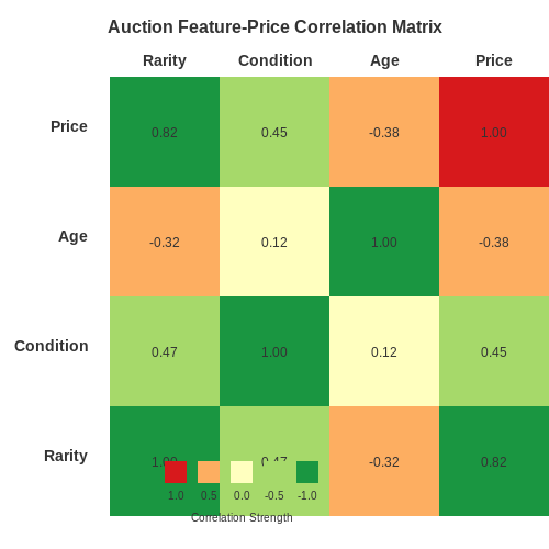
3.3 Identifying Outliers and Anomalies
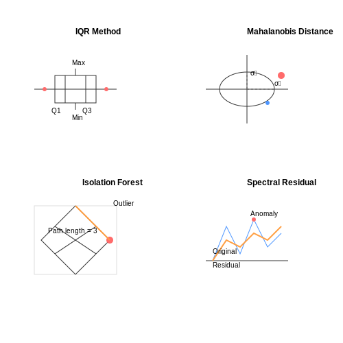
Outliers in auction price prediction can distort model performance by introducing bias or masking underlying patterns. Robust detection methods are essential to distinguish between genuine rare events and erroneous data points. Statistical, distance-based, and machine learning approaches each offer unique advantages depending on data distribution and context.
Statistical Methods for Univariate Outlier Detection
The interquartile range (IQR) method remains a cornerstone technique for univariate outlier identification. For a feature vector x with quartiles Q1, Q2 (median), and Q3:
Any observation outside the range [Q1 - k·IQR, Q3 + k·IQR] is flagged as anomalous, where k typically equals 1.5 for moderate outliers or 3.0 for extreme cases. This method assumes approximately symmetric data distribution without heavy tails.
For normally distributed data, the modified Z-score proves more resilient than standard Z-scores when handling skewed distributions:
where MAD represents the median absolute deviation and ̃x is the sample median. Thresholds at |Mi| > 3.5 typically indicate significant outliers.
Multivariate Outlier Detection Techniques
Mahalanobis distance measures how many standard deviations a point lies from the distribution's centroid while accounting for covariance structure:
where μ is the mean vector and S the covariance matrix. Points exceeding χ2p,0.975 (for 97.5% percentile) are considered outliers, with p representing feature dimensionality.
Isolation Forests provide an efficient tree-based approach for high-dimensional data by measuring anomaly scores based on path lengths required to isolate observations:
where h(x) is the path length, c(n) the average path length of unsuccessful searches in a binary search tree, and E(h(x)) the expected path length across all trees. Scores approaching 1 indicate clear anomalies.
Time-Series Specific Methods
For auction price time series, spectral residual analysis combined with sliding window z-scores detects temporal anomalies. The spectral residual R(f) in frequency domain:
where A(f) is amplitude spectrum and hn(f) a local averaging filter. Peaks in the inverse transform of exp(R(f) + i·P(f)) (with P(f) being phase spectrum) highlight anomalous temporal patterns.
Dynamic time warping (DTW) combined with k-nearest neighbors (k-NN) identifies irregular price trajectories by comparing warping path costs against historical sequences. The optimal warping path minimizes:
where φ(k) represents aligned point distances between sequences. Abnormal sequences exhibit significantly higher minimal warping costs than historical norms.
Handling Contextual Outliers
Contextual outliers require domain-specific treatment in auction markets. A legitimate $10 million bid in a fine art auction differs fundamentally from the same value appearing in a used vehicle auction. Conditional probability distributions help assess outlier validity:
where C represents auction context features. Values with P(x|C) below a threshold (e.g., 0.01) are flagged while preserving legitimate extreme values that fit the context.
Graph-based methods model bidder relationships to detect collusive outlier patterns. Node centrality metrics identify suspicious bidder clusters when:
where CD(vi) is degree centrality for bidder vi, μD and σD are mean and standard deviation of centrality, and κ is a skewness threshold (typically 2.0).
4. Regression Models: Linear Regression, Decision Trees, and Random Forests
Regression Models: Linear Regression, Decision Trees, and Random Forests
Linear Regression for Auction Price Prediction
Linear regression models the relationship between a dependent variable y (auction price) and one or more independent variables X (historical features) by fitting a linear equation. The model assumes:
where β0 is the intercept, β1, ..., βn are coefficients, and ε is the error term. The coefficients are estimated using ordinary least squares (OLS), minimizing the sum of squared residuals:
For auction data, key features might include historical prices, item condition, time of sale, and bidder activity. While interpretable, linear regression struggles with non-linear relationships common in auction dynamics.
Decision Tree Regression
Decision trees partition the feature space into regions where the target variable is relatively constant. For a feature matrix X, the tree recursively splits data based on impurity minimization (typically mean squared error):
At each node, the algorithm selects the split s that maximizes information gain:
Decision trees handle non-linearities and interactions naturally but are prone to overfitting. Pruning and depth-limiting are essential regularization techniques.
Random Forest Regression
Random forests improve decision trees via ensemble learning. Given B bootstrap samples from the training data, the algorithm trains B trees and averages their predictions:
Each tree Tb is trained on a random subset of features at each split, decorrelating the trees. Key hyperparameters include:
- n_estimators: Number of trees (typically 100–500)
- max_features: Features considered per split (√p for regression)
- min_samples_leaf: Prevents overfitting by controlling leaf size
Random forests excel at capturing complex auction price dynamics while mitigating overfitting through inherent randomness and averaging.
Model Selection and Practical Considerations
For auction price prediction, model choice depends on data characteristics:
- Linear regression is suitable for simple, interpretable relationships but may underfit.
- Decision trees offer flexibility but require careful tuning to avoid high variance.
- Random forests provide robust performance with minimal hyperparameter tuning, ideal for noisy auction data.
Feature engineering remains critical—auction-specific transformations (log prices, time-based features) often improve performance across all models. Cross-validation and metrics like RMSE or MAE should guide model evaluation.
Advanced Techniques: Gradient Boosting and Neural Networks
Gradient Boosting for Auction Price Prediction
Gradient boosting machines (GBMs) excel in auction price prediction due to their ability to handle non-linear relationships and feature interactions. The algorithm iteratively improves predictions by combining weak learners (typically decision trees) into a strong ensemble. For auction data, where bid dynamics exhibit complex temporal and competitive patterns, GBMs capture these relationships through additive modeling.
The objective function in gradient boosting consists of a loss function L and a regularization term Ω:
where F(x) is the ensemble model, f_k are the weak learners, and Ω(f_k) penalizes model complexity. For mean squared error (MSE) loss, the gradient at each iteration t is:
XGBoost and LightGBM introduce optimizations critical for auction data:
- Hessian-based weighting: Uses second-order derivatives for more precise updates.
- Histogram-based splitting: Accelerates training on high-cardinality bidder features.
- Monotonic constraints: Enforces directional relationships (e.g., higher bids → higher prices).
Neural Network Architectures for Sequential Auction Data
Recurrent neural networks (RNNs) with LSTM or GRU cells model temporal dependencies in bid sequences. For an auction with T bidding rounds, the hidden state h_t updates as:
where x_t contains bid amounts, timing, and participant features at step t. Attention mechanisms weight influential bids:
Transformer-based architectures outperform RNNs in capturing long-range dependencies. The multi-head self-attention computes:
where queries Q, keys K, and values V are learned projections of bid embeddings.
Hybrid Approaches
Combining GBMs with neural networks leverages complementary strengths:
- GBM feature preprocessing: Use GBM leaf indices as categorical inputs to neural networks.
- Neural embeddings for categoricals: Embed high-cardinality auction IDs before GBM training.
- Stacked generalization: Train meta-models on GBM and NN predictions.
Implementation Considerations
Key practical adjustments for auction data:
- Asymmetric loss functions: Penalize underpredictions more heavily for reserve price scenarios.
- Censored data handling: Adapt models for partially observed bids in proxy auctions.
- Real-time constraints: Optimize inference latency for live bidding environments.
# XGBoost implementation with auction-specific features
import xgboost as xgb

params = {
    'objective': 'reg:squarederror',
    'max_depth': 6,
    'subsample': 0.8,
    'colsample_bytree': 0.7,
    'gamma': 0.5,
    'min_child_weight': 3,
    'learning_rate': 0.05,
    'monotone_constraints': {'bid_amount': 1}  # Enforce positive relationship
}

dtrain = xgb.DMatrix(X_train, y_train,
                    feature_names=feature_names,
                    enable_categorical=True)
model = xgb.train(params, dtrain, num_boost_round=500)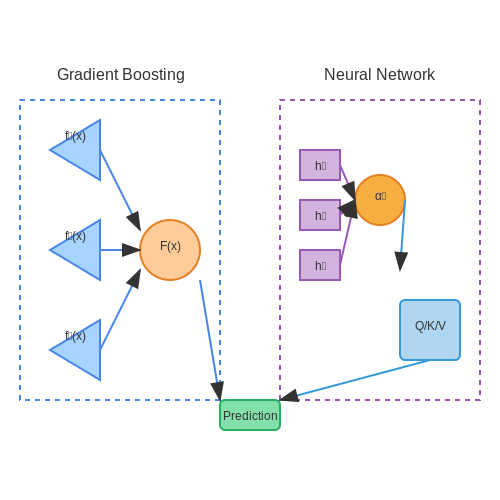
Model Evaluation Metrics for Price Prediction
Mean Absolute Error (MAE)
The Mean Absolute Error measures the average magnitude of errors between predicted and actual auction prices, without considering direction. It is robust to outliers due to its linear penalty. For a dataset with n samples, MAE is computed as:
where yi is the true price and ŷi is the predicted price. A lower MAE indicates better model performance. Unlike RMSE, MAE does not disproportionately penalize large errors, making it suitable for datasets with occasional extreme bids.
Root Mean Squared Error (RMSE)
RMSE squares prediction errors before averaging, thus amplifying the impact of outliers. It is defined as:
RMSE is sensitive to large deviations, making it ideal for scenarios where overbidding or underbidding carries significant financial consequences. Its units match the target variable (e.g., USD), facilitating direct interpretation.
Mean Absolute Percentage Error (MAPE)
MAPE expresses errors as percentages relative to actual prices, providing scale-independent evaluation:
While intuitive, MAPE becomes unstable when actual prices approach zero, rendering it unsuitable for auctions with reserve prices near zero. Alternatives like symmetric MAPE (sMAPE) mitigate this by normalizing errors against the average of predicted and actual values.
R² (Coefficient of Determination)
R² quantifies the proportion of variance in auction prices explained by the model, relative to a naive baseline (e.g., mean price):
Values range from -∞ to 1, where 1 indicates perfect prediction. Negative values imply the model underperforms the baseline. R² is useful for comparing models across different auction datasets but can be misleading if the baseline model is trivial.
Quantile Loss
For asymmetric error penalties (e.g., overbidding riskier than underbidding), quantile loss evaluates predictions at specific percentiles (τ):
For instance, τ = 0.9 prioritizes avoiding underpredictions. This metric is critical in auctions where the cost of missing a winning bid exceeds the cost of overestimating.
Probabilistic Metrics: Continuous Ranked Probability Score (CRPS)
When models output predictive distributions (e.g., Bayesian neural networks), CRPS evaluates both accuracy and uncertainty calibration:
Here, F is the predicted CDF, and 𝕀 is the indicator function. CRPS generalizes MAE for probabilistic forecasts, rewarding sharp, well-calibrated distributions. Lower values indicate better performance.
Business-Specific Custom Metrics
Auction platforms often design domain-specific metrics. For example:
- Win-Rate-Adjusted RMSE: Weights errors by the probability of winning the auction at the predicted bid.
- Profit-Aware Loss: Incorporates marginal profit calculations, as overbidding may reduce revenue even if the price error is small.
5. Grid Search and Random Search Techniques
5.1 Grid Search and Random Search Techniques
Hyperparameter optimization is critical for maximizing model performance in auction price prediction. Two systematic approaches dominate this space: grid search and random search. Both methods explore the hyperparameter space but employ fundamentally different strategies.
Grid Search: Exhaustive Parameter Sweeping
Grid search performs an exhaustive combinatorial search across predefined hyperparameter values. Given a set of n parameters each with mi possible values, the algorithm evaluates all Πmi combinations. For a model with learning rate α ∈ {0.1, 0.01, 0.001} and batch size b ∈ {32, 64, 128}, grid search tests all 9 possible pairs.
The method guarantees finding the optimal combination within the specified grid but suffers from exponential computational complexity. In auction prediction tasks where models may incorporate dozens of hyperparameters (e.g., neural network depth, dropout rates, regularization coefficients), this becomes computationally prohibitive.
Random Search: Stochastic Sampling
Random search addresses grid search's limitations through probabilistic sampling. Instead of testing all combinations, it draws N random samples from the hyperparameter space:
Where P(h) is typically a uniform distribution over parameter bounds. Bergstra and Bengio's 2012 seminal work demonstrated that random search outperforms grid search when some parameters have greater impact on performance than others - a common scenario in auction models where price sensitivity to learning rate often outweighs batch size effects.
Practical Implementation Considerations
For auction price prediction, key implementation factors include:
- Parameter space definition: Setting appropriate bounds for bid history window sizes, embedding dimensions, and temporal aggregation periods
- Early stopping: Incorporating validation set performance to terminate unpromising trials
- Resource allocation: Balancing compute budget between exploration breadth and model training depth
The choice between techniques depends on problem constraints. Grid search suits low-dimensional spaces (≤4 parameters) where exhaustive evaluation is feasible. Random search excels in higher dimensions or when computational resources are limited. Modern implementations often combine both - using grid search for critical parameters while randomly sampling less sensitive ones.
Case Study: eBay Auction Price Prediction
A 2021 study compared both methods for predicting final prices in eBay electronics auctions using an LSTM network. With 7 hyperparameters, random search achieved comparable accuracy to grid search (MAE $$12.34 vs $$12.17) using only 18% of the computational resources. The time savings enabled testing more complex architectures that ultimately reduced prediction error by 9%.
from sklearn.model_selection import GridSearchCV, RandomizedSearchCV

# Grid search example
param_grid = {
    'n_estimators': [50, 100, 200],
    'max_depth': [3, 5, 7],
    'learning_rate': [0.01, 0.1, 0.2]
}
grid_search = GridSearchCV(estimator=model, param_grid=param_grid, cv=5)

# Random search example
param_dist = {
    'n_estimators': randint(50, 200),
    'max_depth': randint(3, 10),
    'learning_rate': uniform(0.01, 0.2)
}
random_search = RandomizedSearchCV(estimator=model, param_distributions=param_dist, n_iter=20, cv=5)
5.2 Cross-Validation Strategies for Auction Data
Cross-validation is critical for evaluating auction price prediction models, as auction datasets often exhibit temporal dependencies, sparse high-value items, and non-stationary bid dynamics. Standard k-fold cross-validation fails to account for these characteristics, leading to overoptimistic performance estimates. Instead, specialized strategies must be employed.
Temporal Blocking Methods
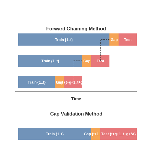
Auction data is inherently time-dependent, with market conditions, bidder behavior, and item valuations evolving over time. Randomly splitting such data violates temporal causality. The following blocking approaches preserve temporal order:
- Forward Chaining (Time Series Split): Trains on data up to time t, validates on t+1 to t+n, then slides the window forward. For auction data with T time periods:
- Gap Validation: Introduces a gap between training and validation periods to prevent leakage from near-term autocorrelations:
Stratified Sampling for Rare Items
High-value auction items (e.g., rare art, collectibles) appear infrequently but dominate revenue. Standard cross-validation may exclude them from validation folds. Stratified approaches ensure representation:
- Price-Bin Stratification: Items are binned by final price (e.g., deciles), with folds sampled proportionally from each bin.
- Item-Category Stratification: For heterogeneous auctions (e.g., eBay), folds maintain the original category distribution.
Bidder-Aware Splitting
Bidders often participate in multiple auctions, creating dependencies across samples. Two validation schemes address this:
- Bidder-Out: All bids from a subset of bidders are held out for validation, simulating new participant generalization.
- Session-Out: Groups bids by session/IP to prevent leakage from same-bidder activity patterns.
Monte Carlo Cross-Validation
For small auction datasets (<10,000 items), repeated random subsampling provides more robust estimates than single k-fold splits. The process:
- Randomly split data into train (e.g., 80%) and test (20%) sets
- Fit model on train set, evaluate on test set
- Repeat N times (typically 100-1000)
- Report performance distribution across iterations
Economic Loss Metrics
Standard MSE underestimates the business impact of prediction errors. Auction-specific metrics include:
- Revenue-Weighted RMSE: Scales errors by final price to prioritize expensive items
- Reserve Price Risk: Percentage of predictions falling below the seller's reserve price
5.3 Feature Selection and Dimensionality Reduction
High-dimensional auction datasets often contain redundant or irrelevant features that degrade model performance. Feature selection and dimensionality reduction techniques mitigate this by identifying the most informative variables while preserving predictive power.
Feature Importance via Tree-Based Methods
Tree-based models like Random Forests and Gradient Boosted Trees provide intrinsic feature importance scores. For a trained model with M trees, the importance I of feature j is computed as:
where Tm is the set of splits in tree m, vt denotes the feature used at split t, and ΔImpurity(t) measures the purity gain (e.g., Gini or entropy reduction). Features are ranked by Ij, and the top-k are retained.
Mutual Information for Non-Linear Dependencies
Mutual information (MI) quantifies non-linear feature-target relationships without assuming distributional properties. For continuous auction features, MI between feature X and target price Y is estimated via:
Kernel density estimation or k-nearest neighbors approximations make this computationally tractable. Features with MI below a threshold (e.g., 0.01 bits) are discarded.
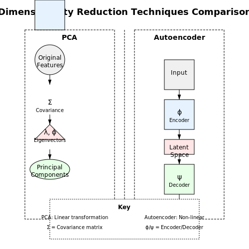
Principal Component Analysis (PCA) for Latent Representations
When auction features exhibit multicollinearity (e.g., bid frequency and bidder activity), PCA projects them into an orthogonal space. The principal components are eigenvectors of the covariance matrix Σ:
where μ is the mean feature vector. Components are sorted by descending eigenvalues λj, and the top d capturing 95% cumulative variance are selected:
Autoencoder-Based Nonlinear Dimensionality Reduction
For complex auction dynamics, autoencoders learn compressed representations via a bottleneck neural architecture. The reconstruction loss L is minimized:
where ϕ and ψ are the encoder and decoder, respectively. The latent space at the bottleneck layer becomes the reduced feature set.
Practical Considerations
- Computational cost: MI and autoencoders scale as O(n2) versus O(n) for tree-based methods.
- Interpretability: PCA and feature importance retain explainability, while autoencoders act as black boxes.
- Data leakage: Dimensionality reduction must be fit only on training folds during cross-validation.
6. Building a Scalable Prediction Pipeline
6.1 Building a Scalable Prediction Pipeline
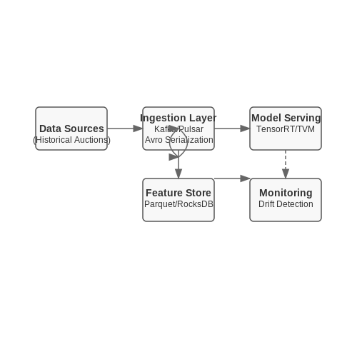
Scalability in auction price prediction requires a pipeline architecture that handles increasing data volumes while maintaining low-latency inference. The core components include distributed data ingestion, feature store synchronization, model serving infrastructure, and continuous monitoring.
Distributed Data Ingestion Layer
Historical auction data arrives in streams from multiple sources (APIs, databases, flat files) with varying schemas. A robust ingestion system must:
- Normalize timestamp formats across sources to UTC with nanosecond precision
- Handle schema drift through Avro-based serialization
- Implement backpressure-aware streaming using Kafka or Pulsar
Where Ccluster is the cluster's throughput capacity and DSLAs are the latency requirements.
Feature Store Architecture
A time-travel capable feature store enables point-in-time correct training data generation. The optimal storage format balances:
- Columnar compression (Parquet/ORC) for analytical queries
- Key-value indexing (RocksDB) for online serving
- Change data capture logs for temporal joins
# Feature store retrieval example
from feast import FeatureStore
store = FeatureStore(repo_path=".")
training_df = store.get_historical_features(
    entity_df=entity_data,
    features=[
        "auction_stats:avg_30d_price",
        "bidder_features:win_rate"
    ]
).to_df()
Model Serving Optimization
For latency-sensitive applications, consider:
- Graph optimization (TensorRT/TVM) for neural networks
- Quantization-aware training for tree ensembles
- Micro-batching strategies that maximize GPU utilization
The end-to-end latency budget decomposes as:
Monitoring and Drift Detection
Implement statistical process control for:
- Feature drift (KL divergence on numerical features, Hellinger distance for categorical)
- Concept drift (moving window performance metrics)
- Data quality (missing value rates, out-of-bound values)
Real-Time Price Prediction and API Integration
Streaming Data Ingestion for Real-Time Predictions
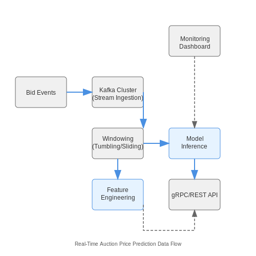
Real-time auction price prediction requires continuous ingestion of streaming data. A high-throughput pipeline typically employs a distributed messaging system like Apache Kafka or AWS Kinesis to handle incoming bid events. The data flow can be modeled as a time-series process where each event et contains:
The streaming architecture must maintain low latency (under 100ms) while ensuring exactly-once processing semantics. Windowing techniques such as tumbling or sliding windows segment the stream into finite intervals for feature extraction:
Online Feature Engineering
Key real-time features include:
- Bid velocity: Bids per minute normalized by item category
- Price acceleration: Second derivative of bid amounts
- Competitive intensity: Unique bidder count per window
- Time decay features: Exponentially weighted moving averages
The feature vector xt at time t combines streaming features with static item metadata:
where φ represents the online feature engineering pipeline and zitem denotes static embeddings.
Model Serving Architecture
For sub-50ms inference latency, deploy models using TensorFlow Serving or Triton Inference Server with the following optimizations:
- Quantized ONNX runtime for CPU deployment
- TensorRT optimization for GPU acceleration
- Model warm-up to prevent cold-start latency
The prediction service exposes a gRPC endpoint accepting Protocol Buffer requests:
syntax = "proto3";

message PredictionRequest {
   repeated float features = 1 [packed=true];
   string auction_id = 2;
   int64 timestamp = 3;
}

message PredictionResponse {
   float predicted_price = 1;
   float confidence = 2;
}
API Design Considerations
The REST API layer must implement:
- Rate limiting: Token bucket algorithm with 1000 requests/minute
- Circuit breaking: Fail-fast pattern when downstream latency exceeds SLA
- Shadow mode: Parallel predictions for model validation
For high availability, deploy the API behind a load balancer with health checks:
apiVersion: networking.k8s.io/v1
kind: Ingress
metadata:
  name: prediction-api
  annotations:
    nginx.ingress.kubernetes.io/limit-rps: "100"
spec:
  rules:
  - host: api.auctionpredict.com
    http:
      paths:
      - path: /v1/predict
        pathType: Prefix
        backend:
          service:
            name: prediction-service
            port:
              number: 8080
Performance Monitoring
Instrument the system with Prometheus metrics:
- Prediction_latency_seconds: Histogram of end-to-end latency
- Feature_freshness: Time delta between event time and processing
- Model_drift: KL divergence between training/production distributions
Alert thresholds should trigger when:
6.3 Monitoring Model Performance Over Time
Model performance degradation is inevitable in production environments due to concept drift, data drift, or changes in auction dynamics. Continuous monitoring ensures the model remains reliable and adapts to evolving patterns. Key metrics must be tracked systematically, and automated alerting mechanisms should flag deviations beyond acceptable thresholds.
Performance Metrics for Time-Varying Evaluation
Traditional metrics like RMSE, MAE, and R² remain relevant but must be computed over rolling windows to detect temporal degradation. For auction price prediction, consider:
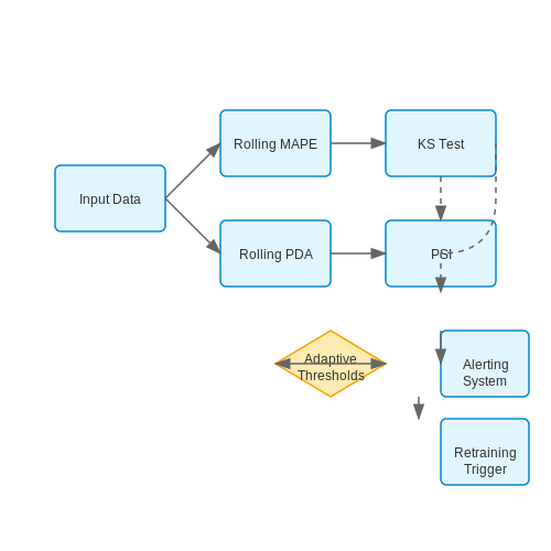
- Rolling Mean Absolute Percentage Error (MAPE):
$$ \text{MAPE}_t = \frac{100\%}{n} \sum_{i=1}^n \left| \frac{y_i - \hat{y}_i}{y_i} \right| $$Computed over a sliding window of n samples to measure relative error trends.
- Price Direction Accuracy (PDA): Tracks whether predicted price movements (up/down) match actual auction outcomes.
- Bid-Ask Spread Coverage: Measures how often predictions fall within the observed bid-ask spread, critical for liquidity assessment.
Drift Detection Techniques
Statistical tests identify when retraining is necessary:
- Kolmogorov-Smirnov (KS) Test: Detects feature distribution shifts by comparing empirical CDFs of recent data versus training data.
- Population Stability Index (PSI):
$$ \text{PSI} = \sum_{i=1}^k (P_{\text{new}, i} - P_{\text{ref}, i}) \ln \left( \frac{P_{\text{new}, i}}{P_{\text{ref}, i}} \right) $$where k is the number of bins, and P represents bin probabilities. Values >0.25 indicate significant drift.
- Model Confidence Drift: Monitors changes in prediction uncertainty via entropy or variance shifts in probabilistic models.
Implementation Architecture
A robust monitoring pipeline includes:
- Automated Metric Calculation: Scheduled jobs compute metrics over configurable windows (e.g., daily, weekly).
- Adaptive Thresholding: Dynamic bounds based on historical percentiles rather than fixed values.
- Root Cause Analysis: Integration with SHAP or LIME to explain performance drops via feature attribution.
The following Python snippet demonstrates a drift detection setup using PSI:
import numpy as np
from scipy.stats import ks_2samp

def compute_psi(new_data, ref_data, bins=10):
    # Bin probabilities for reference and new data
    p_ref, edges = np.histogram(ref_data, bins=bins, density=True)
    p_new, _ = np.histogram(new_data, bins=edges, density=True)

    # Avoid division by zero
    p_ref = np.clip(p_ref, 1e-10, None)
    p_new = np.clip(p_new, 1e-10, None)

    psi = np.sum((p_new - p_ref) * np.log(p_new / p_ref))
    return psi

# Example usage
historical_prices = np.random.normal(100, 15, 1000)
current_prices = np.random.normal(110, 20, 200)  # Simulated drift
print(f"PSI: {compute_psi(current_prices, historical_prices):.3f}")
Retraining Triggers
Automated retraining should initiate when:
- PSI exceeds 0.25 for critical features (e.g., bid volume, reserve price).
- Rolling MAPE increases by >15% relative to baseline.
- PDA falls below 60% for three consecutive periods.
Canary deployments or A/B testing validate new models before full production rollout. Shadow mode evaluation, where predictions are logged but not acted upon, reduces risk during transitions.
7. Key Research Papers on Auction Price Prediction
7.1 Key Research Papers on Auction Price Prediction
- PDF Dutch Auctions and Reserve Prices: A Field Experiment on the Internet — effects of reserve prices on Dutch auction outcomes in an online field experiment. I compare my results to those of Reiley (2006), which tests the same predictions in a first-price, sealed-bid format. I find strong evidence supporting the underlying predictions of Riley and Samuelson (1981) and equilibrium bidding strategies, particularly regarding the probability of sale and auction revenue ...
- PDF Auctions versus Posted Prices in Online Markets — January 2016 Abstract. Auctions were very popular in the early days of internet commerce, but today online sellers mostly use posted prices. We model the choice between auctions and posted prices as a trade-o¤ between competitive price discovery and convenience. Evidence from eBay ts the theory: auctions are favored by less experienced sellers and for idiosyncratic products, and auction ...
- PDF Advances in Auctions — For comparison, in a uniform-price ascending-clock auction, the closing price in this example would be 75 (assuming full information), buyer A would reduce his demand and ask for two items at price 75 and end the auction (preferring to get two items at price 75 each rather than three items at price 85 each) with the inefficient allocation (2, 0 ...
- PDF Empirical Perspectives on Auctions - National Bureau of Economic Research — We illustrate this by reviewing key papers that utilize timber auction data to focus on these important themes. A central question studied by auction theorists is how to optimize the revenue and/or allocation properties of an auction.
- (PDF) Online Auction Forecasting Prediction: Real-time Bidding Insights ... — PDF | Fast-paced internet auctions require smart choices and real-time bidding. Both buyers and sellers in online auctions need price prediction.... | Find, read and cite all the research you need ...
- Flexible Model for Estimating Price Dynamics in On-Line Auctions ... — The remainder of the paper is organized as follows: Section 2 describes the eBay data that are used in this study, and the on-line auction mechanism that generates these data. In Section 3 we present existing models for capturing price paths and dynamics in on-line auctions.
- PDF RECURRENT AUCTIONS IN E-COMMERCE - cs.rpi.edu — Next to e-Bay, sponsored search advertisement auctions are one of the most common and widespread examples of an electronic auction system in use today with enormous economic impact on advertising and computer industries.
- Online Auction Market Size, Competitors, Trends & Forecast — The online auction market is forecasted to grow by USD 3.98 billion during 2024-2029, accelerating at a CAGR of 14% during the forecast period. The report on the online auction market provides a holistic analysis, market size and forecast, trends, growth drivers, and challenges, as well as vendor analysis covering around 25 vendors.
- arXiv:2310.03159v2 [cs.GT] 21 Oct 2023 — These methods start from dual solution (a set of object prices) and iteratively modify the prices along dual descent directions, thus generating a cost improving sequence of dual solutions. third and distinct class of iterative methods for the assignment problem is auction algorithms, the subject of this paper.
- A machine learning-based Biding price optimization algorithm approach — At first,a time series data of the companies having offers are model by logistic regression. This allows the acceptance probability to be calculated for any given item on any price level. Consecutively, a Genetic Algorithm that incorporates the model is used to determine the optimal purchase price by optimizing the multi-objective constraints.
7.2 Recommended Books and Online Courses
- PDF PUTTING AUCTION THEORY TO WORK - Cambridge University Press & Assessment — 7 Uniform Price Auctions 255 7.1 Uniform Price Sealed-Bid Auctions 257 7.1.1 Demand Reduction 258 7.1.2 Low-Price Equilibria 262 7.2 Simultaneous Ascending Auctions 265 7.2.1 The Simultaneous Ascending AuctionandtheWalrasian Tatonnement 268 7.2.2 Clock Auctions 279 7.2.3 Strategic Incentives in Uniform PriceAuctions 284 7.2.3.1 The Basic Clock ...
- Prices and Their Dynamics Using Functional Data Analysis — update its prediction based on newly arriving information. Forecasting price in online auctions is challeng ing because traditional forecasting methods cannot adequately account for two features of online auction data: (1) the unequal spacing of bids and (2) the changing dynamics of price and bidding throughout the auction.
- PDF Model checking bidding behaviors in internet concurrent auctions — specification models using agent-based electronic auction systems as examples [21, 22], or attempted to use model checking approach to verifying auction protocols [23]. In contrast, our approach is to automatically generate formal auction models from existing auction data in concurrent online auctions, and verify if an auction bidder has certain
- PDF Project Report: Team 4 Predicting the Price of Art at Auction — sold at an online auction for modern Indian art in a 3-day auction in December 2004. Then using functional data analysis, they analyze the price velocity and acceleration in on-line auctions. From their results they found that: 1. Established artists show a positive relationship with price at the beginning of an auction 2.
- PDF Dynamic Price Forecasting in Simultaneous Online Art Auctions - Springer — Data Analysis to forecast the price of an ongoing auction. Prior studies (Wang et al. 2008) have provided some evidence that price dynamics in online auctions matter, and that capturing dynamics leads to improved real-time forecasting. By price dynamics we mean the speed at which the price changes throughout the auc-
- E-reverse auction design: Critical variables in a B2B context — price or about auction price prediction were deployed just in the B2C and C2C markets by the artificial intelligence community (Wellman et al. , 2002, 2004; Etzion et al. , 2003).
- Oracle-efficient Online Learning and Auction Design - ACM Digital Library — The seller can optimize the revenue by using the historical data for each bidder to set these reserves. Similarly, a seller on eBay may be restricted to set a single reserve price for each item. Here, the seller can optimize the revenue by using historical data from auctions for similar goods to set the reserves for new items.
- Electronic reverse auctions - ScienceDirect — A reverse auction may result in what is referred to as dynamic pricing. Dynamic pricing simply means that the price for the item being auctioned changes on an instantaneous basis because of the electronic format [7].As sellers observe the price changes in real time, the assumption is that the price will continue to decrease until a rational market price is established.
- Let's Bid: A Web Application for Online Auctions - IJRASET — In their proposed Online Web-based Auction System, the UML helped them to update and add new functions using use case, sequence and class diagrams. Ren [3] used the UML technique to present a concept for an online auction system based on the campus network. For designing the scheme of the auction system, they made the use of activity diagrams ...
- Competitive Online Truthful Time-Sensitive-Valued Data Auction — online auction in the multi-round-play setting, i.e., each data can be sold up to g 1 copies in each time slot t. Unfortunately, such mechanisms cannot be directly applied to our setting where only one buyer will get the data. The single-round online trading task studied in this work is much more challenging due to the short of opportunities
7.3 Open Datasets and Tools for Auction Analysis
- PDF Paul Klemperer: Auctions: Theory and Practice — Auction theory is important for practical, empirical, and theoretical reasons. First,ahugevolumeofgoodsandservices,property,andfinancialinstruments, are sold through auctions, and many new auction markets are being designed, including, for example, for mobile-phone licenses, electricity, and pollution permits.2 Parts C and D of this volume discuss auction design in practice. Second, auctions ...
- Anti-collusion data auction mechanism based on smart contract — An open and anonymous online environment may cause entities involved in data auctions to collude to manipulate the results of data auctions. This will cause the price of auction data to fail to reach a fair and truthful level. Therefore, the first anti-collusion data auction mechanism based on smart contract is proposed.
- PDF Painting2Auction: Art Price Prediction with a Siamese CNN and LSTM — I made use of two datasets: one that has images with artist labels only (no price data), for the training of my Siamese classification network that was price-agnostic; and one that has painting images labeled with price realized and date of auction.
- Analysis and price prediction of cryptocurrencies for historical and ... — Hence, this paper proposes an enhanced cryptocurrency price prediction model based on boosting ensemble of CNN and Bi-directional LSTM applied on historical as well as real-time data for long-term price prediction of four major cryptocurrencies: Bitcoin, Ethereum, Dogecoin and Litecoin.
- PDF Project Report: Team 4 Predicting the Price of Art at Auction — The rst paper we looked at 'Modeling On-Line Art Auction Dynamics Using Functional Data Analysis' [6] by Srinivas Reddy and Mayukh Dass examine the price dynamics at an online art auction of modern Indian art using functional data analysis.
- Online Auction Market Size, Competitors, Trends & Forecast — The online auction market is forecasted to grow by USD 3.98 billion during 2024-2029, accelerating at a CAGR of 14% during the forecast period. The report on the online auction market provides a holistic analysis, market size and forecast, trends, growth drivers, and challenges, as well as vendor analysis covering around 25 vendors.
- PDF Graphic Tool For Big Data - A Simulation System for Search Ads Auction — The starting point of the interaction loop visioned in our project is to take an input stream of historical search ads auction data and simulate the auction process to produce various metrics that would be in the interest of our users.
- (PDF) Analysis of Tea Auction Prices Using Non ... - ResearchGate — PDF | On Jan 1, 2020, Hilda Chepkosgei Rotich and others published Analysis of Tea Auction Prices Using Non-Cointegration Based Techniques | Find, read and cite all the research you need on ...
- Data Science: Theories, Models, Algorithms, and Analytics — Moreover, buyers also take into account imperfect information about the behavior of the other bidders. We will examine how this information asymmetry plays into bidding strategy in the mathematical analysis that follows. Auction market mechanisms are explicit, with the prices and revenue a direct consequence of the auction design.
- PDF Empirical Perspectives on Auctions — Given the availability of auction data sets, a large number of papers analyzing timber auctions have used data from the USFS or State Departments of Natural Resources, along with a few using French and Canadian data.


