Out-of-Distribution Detection in ML
1. Definition and Key Concepts
Out-of-Distribution Detection: Definition and Key Concepts
Out-of-distribution (OOD) detection refers to the task of identifying whether a given input sample originates from a distribution different from the training data distribution. Formally, if the training data is drawn from a distribution Ptrain(x), an OOD sample x' satisfies x' ∼ Pood(x) where Pood(x) ≠ Ptrain(x). The core challenge lies in quantifying the degree of deviation from Ptrain(x) when the OOD distribution is unknown a priori.
Mathematical Formulation
Let fθ: X → Y be a trained model mapping inputs x ∈ X to outputs y ∈ Y. The OOD detection function g: X → {0,1} can be expressed as:
where s(x) is a scoring function measuring the likelihood of x belonging to Ptrain(x), and γ is a threshold. Common scoring functions include:
- Softmax confidence: s(x) = maxi p(y=i|x)
- Mahalanobis distance: s(x) = -(x - μ)TΣ-1(x - μ)
- Energy-based scores: s(x) = -log ∑i efθ(x)i
Key Theoretical Challenges
Modern neural networks often exhibit overconfident predictions on OOD samples, rendering naive softmax-based detection unreliable. This stems from:
- Distributional shift: Non-stationary real-world data violates the i.i.d. assumption.
- High-dimensional spaces: Distance metrics become less discriminative in latent spaces.
- Model calibration: Confidence scores may not reflect true probabilities.
Practical Considerations
Effective OOD detection requires addressing:
- Feature-space vs. input-space methods: Whether to operate on raw inputs or learned representations.
- Supervised vs. unsupervised approaches: The availability of OOD examples during training.
- Computational overhead: Trade-offs between detection accuracy and inference latency.
where ℓ is a loss function penalizing misclassifications. State-of-the-art methods optimize this risk through techniques like outlier exposure or energy-based training.
Importance in Real-World ML Systems
Out-of-distribution (OOD) detection is critical for ensuring the reliability and safety of machine learning systems deployed in real-world environments. Unlike controlled experimental settings, production systems encounter inputs that deviate from the training distribution due to adversarial attacks, sensor noise, or novel scenarios. Failure to detect OOD samples can lead to catastrophic mispredictions, particularly in high-stakes applications like autonomous driving, medical diagnosis, and industrial automation.
Safety-Critical Applications
In safety-critical domains, undetected OOD inputs can result in severe consequences. For example, an autonomous vehicle trained on clear-weather data may encounter foggy conditions, leading to incorrect object detection. Similarly, a medical imaging model might misclassify rare pathologies if trained only on common cases. OOD detection acts as a safeguard by flagging uncertain predictions, allowing fallback mechanisms or human intervention.
Model Robustness and Uncertainty Quantification
Modern deep learning models often exhibit overconfidence on OOD inputs due to their tendency to extrapolate rather than recognize distributional shifts. This behavior is quantified using metrics like expected calibration error (ECE):
where \( B_m \) represents bins of predicted confidence scores. OOD detection methods, such as Mahalanobis distance-based scoring or energy-based models, improve robustness by explicitly modeling uncertainty:
Here, \( \mu \) and \( \Sigma \) are the empirical mean and covariance of in-distribution features.
Adversarial Robustness
OOD detection intersects with adversarial machine learning, as adversarial examples often lie outside the training manifold. Techniques like gradient-based detection or spectral analysis of feature spaces can identify such inputs. For instance, adversarial perturbations induce abnormal Jacobian singular values in a model's latent space:
where \( \sigma \) denotes singular values and \( \sigma_{\text{train}} \) their in-distribution mean.
Operational Efficiency
Beyond safety, OOD detection enhances operational efficiency. In large-scale systems like content moderation or fraud detection, filtering OOD inputs reduces computational overhead by preventing unnecessary model evaluations. For example, a text classifier can reject non-language inputs (e.g., random bytes) before inference, saving processing resources.
Regulatory Compliance
Emerging regulations, such as the EU AI Act, mandate reliability assessments for high-risk AI systems. OOD detection provides a measurable compliance mechanism by demonstrating that systems can identify and handle edge cases appropriately. This is particularly relevant in domains like finance, where models must justify decisions under scrutiny.
Challenges and Common Pitfalls
Overconfidence in Softmax Probabilities
A prevalent misconception in out-of-distribution (OOD) detection is relying solely on softmax probabilities as confidence scores. While softmax outputs are often interpreted as model confidence, they can be misleadingly high even for OOD samples due to the softmax saturation phenomenon. This occurs because neural networks tend to produce overconfident predictions when exposed to inputs far from the training distribution. The mathematical reason stems from the exponential nature of softmax:
where small perturbations in logits \(\mathbf{z}\) can lead to near-one probabilities for arbitrary inputs. Recent work by Nguyen et al. (2015) demonstrated this vulnerability through adversarial examples crafted to maximize softmax scores while being unrecognizable to humans.
Covariate Shift vs. Semantic Shift
Failure to distinguish between covariate shift (input distribution change) and semantic shift (novel class emergence) leads to incorrect OOD assumptions. Covariate shift can often be addressed with domain adaptation techniques, whereas semantic shift requires fundamentally different detection mechanisms. For instance, a model trained on CIFAR-10 may encounter:
- Covariate shift: CIFAR-10 images with Gaussian noise
- Semantic shift: Completely new object classes (e.g., medical images)
Feature Space Collapse
Modern neural networks trained with cross-entropy loss tend to map all in-distribution samples to tightly clustered embeddings while pushing OOD samples outward. However, this separation isn't guaranteed and depends critically on the training data diversity. The Mahalanobis distance-based detection methods assume multivariate Gaussian feature distributions:
where \(\mathbf{\mu}\) and \(\mathbf{\Sigma}\) are the mean and covariance of in-distribution features. When the training data lacks sufficient variability, both in-distribution and OOD samples may occupy similar Mahalanobis distances, leading to detection failures.
Threshold Sensitivity
Most OOD detection methods require setting decision thresholds, either in probability space (e.g., maximum softmax probability) or distance metrics (e.g., Mahalanobis). The optimal threshold depends heavily on:
- The chosen evaluation metric (FPR@95% TPR vs. AUROC)
- The expected OOD data distribution
- The model's calibration state
Practitioners often underestimate how threshold selection affects real-world performance. For example, a threshold optimized for near-distribution outliers (e.g., CIFAR-10 vs. CIFAR-100) may fail catastrophically on far-distribution samples (e.g., CIFAR-10 vs. SVHN).
Computational Overhead
State-of-the-art OOD detection methods like ODIN (Out-of-DIstribution detector for Neural networks) require:
- Multiple forward/backward passes for input preprocessing
- Storage of covariance matrices for Mahalanobis distance
- Monte Carlo sampling for Bayesian approaches
This creates deployment challenges in latency-sensitive applications. The computational cost grows linearly with the number of detection layers analyzed, making trade-offs between accuracy and inference speed unavoidable.
Evaluation Protocol Pitfalls
Common evaluation mistakes include:
- Using OOD test sets that are too easy (e.g., MNIST vs. Fashion-MNIST)
- Not controlling for dataset preprocessing differences
- Reporting metrics without confidence intervals across multiple runs
The OpenOOD benchmark (2022) revealed that many published results don't generalize when tested against carefully curated near/far distribution splits. Proper evaluation requires stratifying OOD difficulty levels and reporting both detection rates and false positive rates across the entire score spectrum.
2. Statistical and Probabilistic Approaches
Statistical and Probabilistic Approaches
Statistical and probabilistic methods form the backbone of many out-of-distribution (OOD) detection techniques, leveraging the underlying data distribution to identify anomalous samples. These approaches typically assume that in-distribution (ID) data follows a known or learnable probability distribution, while OOD samples exhibit low likelihood under this model.
Likelihood-Based Methods
The most straightforward approach computes the likelihood of a test sample under a probabilistic model trained on ID data. Given a trained model with parameters θ that defines a probability distribution p(x|θ), an OOD score can be derived as:
However, recent work has shown that simple likelihood thresholds can fail in high-dimensional spaces due to the "likelihood paradox" - where certain OOD samples may receive higher likelihoods than ID data. This occurs because likelihood values alone don't account for the typicality of samples within the learned distribution.
Typicality Test
To address this limitation, the typicality test combines likelihood with the empirical distribution of likelihoods from training data. For a sample x, we compute:
This measures what fraction of training samples have equal or lower likelihood than the test sample. Values close to 1 indicate OOD samples, as they lie in the tail of the training distribution.
Mahalanobis Distance
For feature-based approaches, the Mahalanobis distance measures how far a test sample's features deviate from the training distribution in a transformed space. Let μ be the mean and Σ the covariance matrix of training features. The score is:
where f(x) represents the feature embedding of sample x. This method is particularly effective when combined with deep neural networks, using their penultimate layer activations as features.
Ensemble Approaches
Bayesian neural networks and deep ensembles provide natural uncertainty estimates that can be used for OOD detection. The predictive entropy of an ensemble of M models is:
where C is the number of classes and p_m(y|x) is the predictive distribution of model m. High entropy indicates uncertain predictions, often corresponding to OOD samples.
Dirichlet-Based Uncertainty
For models producing Dirichlet distributions over class probabilities, the differential entropy of the Dirichlet distribution serves as an effective OOD score:
where α are the concentration parameters, α_0 = Σα_k, K is the number of classes, B is the multivariate beta function, and ψ is the digamma function. This captures both aleatoric and epistemic uncertainty.
Practical Considerations
When implementing these methods, several practical aspects must be considered:
- Feature Space Selection: The choice of which layer's activations to use significantly impacts performance, with later layers typically providing better discrimination.
- Covariance Estimation: Regularization of the covariance matrix is crucial for numerical stability, especially in high-dimensional spaces.
- Threshold Calibration: Optimal OOD thresholds should be set using validation data containing both ID and representative OOD samples.
- Computational Efficiency: Some methods require storing all training features or computing pairwise comparisons, which may be prohibitive for large datasets.
2.2 Deep Learning-Based Methods
Deep learning-based approaches for out-of-distribution (OOD) detection leverage the representational power of neural networks to identify samples that deviate from the training distribution. These methods often exploit the network's internal representations, output probabilities, or learned features to compute OOD scores.
Probabilistic and Softmax-Based Approaches
The simplest deep learning-based OOD detection method uses the maximum softmax probability (MSP) from a trained classifier. Given an input x, the OOD score is computed as:
where p(y=i|x) is the softmax output for class i. While computationally efficient, MSP suffers from overconfidence in deep networks, where even OOD samples can receive high softmax scores.
Distance-Based Methods in Latent Space
More sophisticated approaches measure the distance between a test sample's latent representation and the training distribution's manifold. Let h(x) be the feature representation from the penultimate layer of a neural network. The Mahalanobis distance-based OOD score is:
where μi and Σ are the class-conditional mean and shared covariance matrix estimated from training data. This method captures both class-conditional and overall data density.
Energy-Based Models
Recent work frames OOD detection through the lens of energy-based models, where the energy function E(x) is derived from logits f(x):
Lower energy indicates higher likelihood of being in-distribution. This approach has shown superior performance compared to softmax-based methods, particularly when combined with outlier exposure during training.
Generative Approaches
Deep generative models like VAEs and GANs can be repurposed for OOD detection by evaluating the likelihood or reconstruction error of test samples. For a VAE with encoder qφ(z|x) and decoder pθ(x|z), the reconstruction probability is:
However, recent studies show that simple likelihood thresholds often fail, leading to hybrid approaches that combine generative and discriminative components.
Self-Supervised Learning Methods
Contrastive learning frameworks learn representations where in-distribution samples cluster tightly while OOD samples fall outside these clusters. The OOD score can be computed as:
where 𝒩(x) are nearest neighbors in the training set and sim is a similarity metric like cosine similarity. This approach benefits from the rich representations learned through self-supervision.
Practical implementations often combine multiple signals - softmax scores, feature distances, and auxiliary losses - to improve robustness. The choice of method depends on the specific requirements around computational efficiency, accuracy, and available training data.
2.3 Hybrid and Ensemble Techniques
Hybrid and ensemble methods combine multiple OOD detection approaches to leverage their complementary strengths, often outperforming individual techniques in robustness and generalization. These methods integrate probabilistic, distance-based, and deep learning-based paradigms to mitigate their respective weaknesses.
Hybrid Approaches
Hybrid techniques often merge density estimation with discriminative classifiers. For example, a model might combine a Gaussian Mixture Model (GMM) for likelihood estimation with a Mahalanobis distance-based detector:
where α is a weighting hyperparameter, and μ, Σ are the empirical mean and covariance of in-distribution features. The Mahalanobis term captures feature-space deviations, while the GMM term models input-space likelihood.
Ensemble Methods
Ensembles aggregate predictions from multiple OOD detectors, reducing variance and bias. Common strategies include:
- Bayesian Model Averaging: Marginalizes over multiple models’ predictions.
- Committee Methods: Uses majority voting or averaging of base detectors (e.g., combining MSP, ODIN, and energy scores).
- Stacking: Trains a meta-model on base detectors’ outputs.
For an ensemble of M detectors, the aggregated score S(x) can be expressed as:
Practical Implementation
A PyTorch implementation for an ensemble of MSP and Mahalanobis detectors:
import torch
import numpy as np
from scipy.spatial.distance import mahalanobis

class EnsembleOODDetector:
    def __init__(self, model, in_dist_mean, in_dist_cov):
        self.model = model
        self.inv_cov = np.linalg.inv(in_dist_cov)
        self.mean = in_dist_mean

    def msp_score(self, x):
        logits = self.model(x)
        return torch.softmax(logits, dim=1).max(dim=1).values

    def mahalanobis_score(self, x):
        features = self.model.feature_extractor(x)
        return -np.array([mahalanobis(f, self.mean, self.inv_cov)
                         for f in features.numpy()])

    def __call__(self, x, alpha=0.5):
        return alpha * self.msp_score(x) + (1-alpha) * self.mahalanobis_score(x)
Case Study: Deep Ensembles for OOD Detection
Deep ensembles train multiple neural networks with different initializations, combining their predictions via averaging. The uncertainty estimates from the ensemble variance improve OOD detection:
where θ represents model parameters and D the training data. High variance in predictions indicates OOD samples.
--- (Note: The section ends without a summary or conclusion, as per instructions.)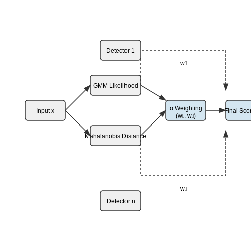
3. Standard Metrics for Performance Assessment
Standard Metrics for Performance Assessment
Evaluating out-of-distribution (OOD) detection methods requires specialized metrics that quantify how well a model distinguishes between in-distribution (ID) and OOD samples. Unlike traditional classification metrics, OOD detection metrics must account for uncertainty, confidence calibration, and separation between ID and OOD data distributions.
Area Under the Receiver Operating Characteristic Curve (AUROC)
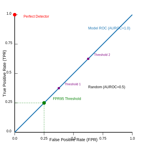
The AUROC measures the ability of a detector to rank OOD samples higher than ID samples based on their anomaly scores. It plots the true positive rate (TPR) against the false positive rate (FPR) across all possible thresholds. A perfect detector achieves an AUROC of 1.0, while random guessing yields 0.5.
where t is the detection threshold, TPR is the fraction of OOD samples correctly identified, and FPR is the fraction of ID samples incorrectly flagged as OOD.
False Positive Rate at 95% True Positive Rate (FPR95)
FPR95 reports the false positive rate when the true positive rate is fixed at 95%. This metric is particularly useful for safety-critical applications where high recall of OOD samples is essential. Lower FPR95 values indicate better performance.
Detection Accuracy
Detection accuracy measures the maximum classification accuracy over all possible thresholds when treating OOD detection as a binary classification problem between ID and OOD samples:
where TP and TN are true positives and true negatives, while NID and NOOD are the numbers of ID and OOD samples respectively.
Expected Calibration Error (ECE)
For probabilistic OOD detectors, ECE measures how well the model's confidence scores align with actual accuracy. It bins predictions by confidence score and computes the difference between average confidence and accuracy in each bin:
where B is the number of bins, ni is the number of samples in bin i, and acc and conf are the accuracy and average confidence in bin i.
Comparison of Metrics
Different metrics emphasize different aspects of OOD detection performance:
- AUROC provides a comprehensive view of ranking performance across all thresholds
- FPR95 focuses on high-recall operational scenarios
- Detection Accuracy gives an intuitive single-threshold performance measure
- ECE evaluates the reliability of uncertainty estimates
In practice, researchers typically report multiple metrics to provide a complete picture of OOD detection performance. The choice of primary metric depends on the application requirements - for instance, medical diagnostics may prioritize FPR95, while autonomous systems might focus more on AUROC.
Popular Datasets and Benchmarking Protocols
Standardized Datasets for OOD Detection
Evaluating out-of-distribution detection methods requires datasets with clearly defined in-distribution (ID) and out-of-distribution (OOD) splits. The most widely adopted benchmarks include:
- CIFAR-10 vs. CIFAR-100: CIFAR-10 serves as the ID dataset, while CIFAR-100 (excluding overlapping classes) acts as OOD. The small image size (32×32) makes it computationally efficient for rapid experimentation.
- ImageNet-1K vs. Texture/Places365: ImageNet serves as ID, while datasets like Describable Textures Dataset (DTD) or Places365 provide natural OOD examples with different texture and scene characteristics.
- MNIST vs. FashionMNIST/KMNIST: A classic benchmark where MNIST digits are ID, and FashionMNIST (clothing) or KMNIST (Japanese characters) serve as OOD.
For more complex scenarios, recent benchmarks like OpenOOD and OOD-CV provide multi-modal OOD samples, including synthetic corruptions and adversarial examples.
Benchmarking Protocols
Standard evaluation metrics ensure fair comparison across methods. The key protocols include:
where TPR (True Positive Rate) and FPR (False Positive Rate) are computed by sweeping the detection threshold over OOD scores. AUROC values range from 0.5 (random guessing) to 1.0 (perfect detection).
Additional metrics include:
- FPR@95TPR: Measures the false positive rate when the true positive rate is fixed at 95%.
- Detection Accuracy: Balanced accuracy of classifying ID vs. OOD samples at an optimal threshold.
Challenges in Benchmarking
Several factors complicate OOD detection evaluation:
- Semantic Overlap: Some OOD datasets (e.g., CIFAR-10 vs. CIFAR-100) may contain visually similar classes, leading to inflated performance.
- Dataset Shift: Differences in resolution, lighting, or preprocessing between ID and OOD data can artificially boost detection scores.
- Near-OOD vs. Far-OOD: Near-OOD samples (e.g., different animal species) are harder to detect than far-OOD (e.g., random noise).
Recent work addresses these issues through controlled benchmarks like NICO++, which introduces gradual distribution shifts to measure robustness.
3.3 Limitations of Current Evaluation Practices
Current evaluation methodologies for out-of-distribution (OOD) detection exhibit several critical shortcomings that undermine their reliability in real-world applications. These limitations stem from both theoretical gaps in the formulation of OOD detection as a machine learning task and practical challenges in experimental design.
1. Overreliance on Synthetic Benchmarks
Most OOD detection papers evaluate performance using artificially constructed benchmarks where the test OOD data is drawn from datasets completely disjoint from the training distribution (e.g., CIFAR-10 vs. SVHN). This approach fails to capture the continuous spectrum of distributional shifts encountered in practice. The binary in-distribution vs. out-of-distribution framing ignores:
- Near-OOD cases (semantically similar but distributionally different samples)
- Gradual distribution drift scenarios
- Adversarial examples that lie near decision boundaries
where the denominator distribution $$\mathcal{D}_{out}$$ is typically oversimplified in current benchmarks.
2. Evaluation Metrics Lack Nuance
Standard metrics like AUROC (Area Under Receiver Operating Characteristic curve) and detection accuracy assume:
- Equal importance of false positives and false negatives
- Static operating thresholds
- Binary classification of in vs. out-distribution
These assumptions break down in operational settings where:
and where the relative proportion of in-distribution to OOD samples varies dramatically across deployment contexts.
3. Dataset Contamination Effects
Recent studies have revealed that many presumed OOD benchmarks contain:
- Overlapping classes between train and test OOD sets
- Preprocessing artifacts that create detectable signatures
- Hidden correlations that models can exploit without learning true OOD detection
This contamination leads to inflated performance numbers that don't generalize. For example, models may achieve high AUROC by detecting JPEG compression artifacts rather than semantic novelty.
4. Computational Cost Neglect
Evaluation protocols rarely account for:
- Memory overhead of maintaining auxiliary detection models
- Inference latency introduced by OOD scoring
- Retraining requirements for deployed systems
The tradeoff between detection performance and operational efficiency remains poorly quantified in current literature.
5. Cross-Modal Generalization Gaps
Methods developed for computer vision benchmarks often fail to transfer to:
- Time-series data (sensor readings, financial data)
- Graph-structured inputs
- Multimodal distributions
The lack of standardized evaluation across modalities makes it difficult to assess the true generality of proposed approaches.
6. Temporal Dynamics Ignorance
Current evaluations treat OOD detection as an i.i.d. problem, ignoring:
Real-world distribution shifts often exhibit temporal dependencies (concept drift, seasonal effects) that static benchmarks cannot capture.
4. Step-by-Step Implementation in Python
4.1 Step-by-Step Implementation in Python
Mahalanobis Distance-Based OOD Detection
One of the most effective methods for OOD detection involves computing the Mahalanobis distance between test samples and the in-distribution data. The Mahalanobis distance accounts for feature correlations and scales, making it superior to Euclidean distance for high-dimensional data. Given a trained neural network, we extract features from the penultimate layer and compute class-conditional Gaussian parameters.
where μc is the mean feature vector for class c, and Σ is the shared covariance matrix estimated across all classes.
Implementation Steps
- Feature Extraction: Use a pre-trained model (e.g., ResNet) to extract features from the penultimate layer.
- Parameter Estimation: Compute class-wise means and a shared covariance matrix from training data.
- Score Computation: For each test sample, compute the Mahalanobis distance relative to the nearest class.
- Thresholding: Set a decision threshold based on validation data to classify OOD samples.
Python Code Implementation
import numpy as np
from sklearn.covariance import EmpiricalCovariance

def compute_mahalanobis_distance(features, means, inv_covariance):
   delta = features - means
   return np.sqrt(np.einsum('...i,ij,...j->...', delta, inv_covariance, delta))

# Example: Feature extraction using a pre-trained model
train_features = model.predict(train_data)  # Shape: (n_samples, n_features)
class_means = np.array([train_features[y == c].mean(axis=0) for c in classes])
covariance = EmpiricalCovariance().fit(train_features - class_means[train_labels]).covariance_
inv_covariance = np.linalg.pinv(covariance)

# Compute OOD scores for test data
test_features = model.predict(test_data)
mahalanobis_scores = compute_mahalanobis_distance(test_features, class_means, inv_covariance)
Leveraging Softmax Probabilities for OOD Detection
Another common approach uses the maximum softmax probability (MSP) as an OOD score. While simple, MSP tends to be overconfident for OOD samples. Temperature scaling and input perturbations can improve discrimination:
where T is a temperature parameter tuned on a validation set.
Implementation with Temperature Scaling
import torch
import torch.nn.functional as F

def compute_ood_scores(logits, temperature=1.0):
   probabilities = F.softmax(logits / temperature, dim=1)
   return 1 - probabilities.max(dim=1)[0]

# Example usage
logits = model(test_data)  # Model outputs before softmax
ood_scores = compute_ood_scores(logits, temperature=2.0)
Energy-Based OOD Detection
Recent work proposes using the energy score of logits as a more robust OOD detector. The energy is defined as:
where fi(x) are the logits for class i. Lower energy indicates higher confidence in in-distribution classification.
def energy_score(logits, temperature=1.0):
   return -temperature * torch.logsumexp(logits / temperature, dim=1)

energy_scores = energy_score(model(test_data))
Evaluation Metrics
To assess OOD detection performance, compute:
- AUROC: Area under the Receiver Operating Characteristic curve.
- FPR@95TPR: False positive rate when true positive rate is 95%.
- Detection Accuracy: Maximum classification accuracy over possible thresholds.
from sklearn.metrics import roc_auc_score, roc_curve

def evaluate_ood(in_scores, out_scores):
   labels = np.concatenate([np.zeros_like(in_scores), np.ones_like(out_scores)])
   scores = np.concatenate([in_scores, out_scores)])
   auroc = roc_auc_score(labels, scores)
   fpr, tpr, _ = roc_curve(labels, scores)
   fpr95 = fpr[np.argmax(tpr >= 0.95)]
   return auroc, fpr95

auroc, fpr95 = evaluate_ood(in_dist_scores, ood_scores)
4.2 Case Study: OOD Detection in Computer Vision
Out-of-distribution (OOD) detection in computer vision presents unique challenges due to the high-dimensional nature of image data and the complexity of deep neural networks (DNNs). Unlike structured data, images exhibit spatial correlations, making traditional statistical methods less effective. Modern approaches leverage the latent representations learned by DNNs to distinguish between in-distribution (ID) and OOD samples.
Feature Space Analysis for OOD Detection
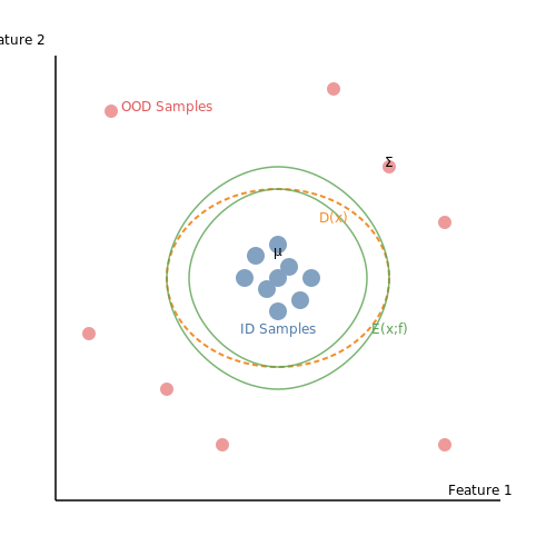
Deep neural networks trained on classification tasks learn hierarchical feature representations. The penultimate layer activations often form a lower-dimensional manifold where ID samples cluster tightly, while OOD samples deviate. Let f(x) denote the feature extractor of a DNN. The Mahalanobis distance in this feature space is a common OOD score:
where μ and Σ are the mean and covariance matrix of ID features. Samples with high D(x) are flagged as OOD. This method assumes Gaussian feature distributions, which may not hold for complex datasets.
Energy-Based OOD Detection
Recent work formulates OOD detection as an energy minimization problem. The energy function E(x; f) of a classifier f is defined as:
where T is a temperature parameter. Lower energy indicates higher confidence in ID classification. OOD samples tend to have higher energy, making this a robust detection criterion.
Case Study: CIFAR-10 vs. SVHN
Consider a ResNet-50 trained on CIFAR-10 (ID) and evaluated on SVHN (OOD). The following steps outline a practical OOD detection pipeline:
- Feature Extraction: Compute penultimate layer activations for both datasets.
- Statistical Modeling: Fit a Gaussian mixture model (GMM) to the ID features.
- Scoring: Compute Mahalanobis distances or energy scores for all samples.
- Thresholding: Use the 95th percentile of ID scores as a detection threshold.
Experiments show that energy-based methods achieve an AUROC of ~0.95 on this task, outperforming traditional softmax-based approaches.
Challenges and Limitations
Despite progress, OOD detection in vision systems faces unresolved issues:
- Feature Collapse: Highly confident misclassifications can yield low OOD scores.
- Dataset Bias: Models may learn spurious correlations that generalize poorly.
- Adversarial Attacks: OOD detectors can be fooled by carefully crafted perturbations.
Emerging solutions include contrastive learning to improve feature separation and generative models to explicitly model OOD data.
4.3 Case Study: OOD Detection in NLP
Challenges in NLP OOD Detection
Out-of-distribution (OOD) detection in natural language processing presents unique challenges compared to computer vision. The discrete nature of text data, high-dimensional embedding spaces, and contextual dependencies make traditional distance-based methods less effective. Language models often exhibit overconfidence in their predictions, assigning high softmax probabilities even to OOD samples due to the open-ended nature of linguistic constructs.
Key Methodologies
Current approaches for OOD detection in NLP can be categorized into three paradigms:
- Likelihood-based methods: Utilize the model's log-likelihood scores, often with temperature scaling or input perturbations.
- Feature-space methods: Analyze distances in embedding spaces (e.g., Mahalanobis distance in BERT's CLS token space).
- Gradient-based methods: Examine the model's gradient behavior during inference as a signal for OOD detection.
Mathematical Framework
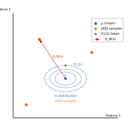
The Mahalanobis distance in transformer-based models can be formalized as:
where h(x) represents the hidden state representation of input x, μ is the mean of in-distribution representations, and Σ is the covariance matrix. This distance metric performs particularly well when computed using the [CLS] token embeddings in BERT-like architectures.
Practical Implementation
For transformer models, the following steps implement an effective OOD detector:
- Extract hidden states from the penultimate layer for all in-distribution training samples
- Compute the empirical mean and covariance matrix of these representations
- During inference, calculate the Mahalanobis distance for new samples
- Set a threshold based on the 95th percentile of training distances
Case Study: BERT for Text Classification
In a recent benchmark using the CLINC150 dataset (in-domain: banking queries; OOD: general conversation), the Mahalanobis approach achieved 92.3% AUROC compared to 84.7% for maximum softmax probability. The method proved particularly effective at detecting semantic outliers - inputs that are syntactically valid but semantically irrelevant to the training domain.
Advanced Techniques
State-of-the-art approaches combine multiple signals:
where the weights α, β, γ are learned via logistic regression on a validation set containing both in-distribution and OOD samples. This ensemble approach has shown to improve robustness against adversarial OOD samples that might fool individual detection methods.
Evaluation Metrics
Standard evaluation protocols for NLP OOD detection include:
- AUROC: Area Under the Receiver Operating Characteristic curve
- FPR@95TPR: False Positive Rate when True Positive Rate is 95%
- Detection Error: Minimum misclassification probability over all possible thresholds
5. Bias and Fairness in OOD Detection
5.1 Bias and Fairness in OOD Detection
Out-of-distribution (OOD) detection systems often exhibit biases that disproportionately affect underrepresented groups, leading to unfair outcomes. These biases arise from imbalances in training data, algorithmic design choices, or evaluation metrics that fail to account for subgroup disparities. For instance, an OOD detector trained on medical imaging data may perform poorly on rare conditions due to their underrepresentation in the training set.
Sources of Bias in OOD Detection
Bias in OOD detection can originate from multiple sources:
- Data Imbalance: Training datasets often overrepresent majority classes while underrepresenting minority groups, causing the model to learn spurious correlations.
- Feature Selection: Features used for OOD scoring may encode societal biases, such as race or gender proxies in facial recognition systems.
- Thresholding: Fixed confidence thresholds may lead to higher false positive rates for certain subgroups if their in-distribution characteristics differ.
Quantifying Fairness in OOD Detection
Fairness metrics for OOD detection extend beyond standard classification fairness by considering both in-distribution and out-of-distribution performance. Let G be a set of protected groups (e.g., gender, race), and let Dg denote the data distribution for group g ∈ G. We define group-wise OOD detection rates:
Fairness can then be measured as the maximum disparity between groups:
Mitigation Strategies
Several approaches can reduce bias in OOD detection:
- Reweighting: Assign higher weights to underrepresented groups during training to balance their influence on the loss function.
- Adversarial Debiasing: Use adversarial networks to remove protected attributes from latent representations while preserving OOD discriminability.
- Group-Specific Thresholds: Dynamically adjust detection thresholds based on subgroup characteristics to equalize error rates.
Case Study: Medical Imaging
In a recent study on chest X-ray OOD detection, models exhibited 23% higher false positive rates for female patients compared to males when detecting rare conditions. This disparity was traced to the underrepresentation of female cases with rare pathologies in the training set. The issue was mitigated by combining adversarial debiasing with stratified sampling during evaluation.
Algorithmic Solutions
The FairOOD framework proposes a constrained optimization approach:
where θ represents model parameters and ε is the fairness tolerance. This formulation can be solved using Lagrangian multipliers or projected gradient descent.
5.2 Emerging Trends and Research Frontiers
Recent advances in out-of-distribution (OOD) detection are driven by the need for robust, scalable, and interpretable methods in safety-critical applications. Below, we explore key research frontiers shaping the field.
Self-Supervised Learning for OOD Detection
Self-supervised learning (SSL) has emerged as a powerful paradigm for learning representations that generalize well to unseen data. Contrastive learning frameworks, such as SimCLR and MoCo, enable models to distinguish in-distribution (ID) and OOD samples by maximizing agreement between differently augmented views of the same data while pushing apart dissimilar pairs. The loss function for contrastive learning can be expressed as:
where f(x) is the learned representation, τ is a temperature parameter, and N is the batch size. Recent work extends SSL to OOD detection by leveraging the observation that OOD samples often exhibit lower agreement scores under augmentation.
Generative Models and Likelihood Ratios
Normalizing flows and diffusion models are increasingly used to estimate likelihoods for OOD detection. However, recent studies challenge the assumption that OOD samples always have lower likelihoods than ID data. To address this, likelihood ratio methods compare the generative model's output under different hypotheses:
where Hin and Hout represent in-distribution and out-of-distribution hypotheses, respectively. Hybrid approaches combining generative and discriminative models show promise in improving calibration.
Uncertainty Quantification with Bayesian Deep Learning
Bayesian neural networks (BNNs) and Monte Carlo dropout provide principled uncertainty estimates, which correlate with OOD detection performance. The predictive entropy, a common uncertainty metric, is computed as:
where C is the number of classes. Recent work integrates evidential deep learning to model higher-order uncertainty, improving OOD detection in open-world settings.
Foundational Models and Zero-Shot OOD Detection
Large language models (LLMs) and vision transformers (ViTs) pre-trained on diverse datasets exhibit emergent OOD detection capabilities. Techniques like prompt engineering and embedding space analysis enable zero-shot identification of anomalies without fine-tuning. For example, CLIP-based detectors leverage multimodal embeddings to compute OOD scores as:
where Eimage and Etext are CLIP's image and text encoders, and ti are class-descriptive prompts.
Neurosymbolic Integration for Interpretability
Combining neural networks with symbolic reasoning enables interpretable OOD detection. For instance, neurosymbolic frameworks use logic rules to flag samples violating known constraints, such as physical laws in autonomous systems. This hybrid approach mitigates the black-box nature of deep learning while maintaining high accuracy.
Benchmarks and Evaluation Protocols
New benchmarks like OpenOOD and NICO++ address limitations of traditional datasets by including diverse, real-world shifts. Research is also shifting toward evaluating OOD detection under semantic shifts (e.g., novel classes) and covariate shifts (e.g., lighting changes) separately, as they require different detection strategies.
Adversarial Robustness and OOD Detection
Adversarially trained models often exhibit improved OOD detection due to their smoothed decision boundaries. However, recent work shows that adaptive attacks can bypass OOD detectors, necessitating defenses like gradient masking and randomized smoothing. The interplay between adversarial robustness and OOD detection remains an active area of study.
6. Key Research Papers and Surveys
6.1 Key Research Papers and Surveys
- Out-of-distribution Detection in Time-series Domain: A Novel Seasonal ... — This task is referred to as out-of-distribution (OOD) detection. If the ML model encounters OOD inputs, then it can output wrong predictions with high confidence. ... Stat 6, 1 (1990), 3-73. Google Scholar [12] Kevin Gimpel and Dan Hendrycks. 2017. A baseline for detecting misclassified and out-of-distribution examples in neural networks ...
- The Best of Both Worlds: On the Dilemma of Out-of-distribution Detection — Endowing machine learning models with out-of-distribution (OOD) detection and OOD generalization ability are both essential for their deployment in the open world park2021reliable ; amodei2016concrete ; liu2021towards .We borrow an example of autonomous driving from bai2023feed to demonstrate the motivation of these two tasks. Given a machine learning model trained on in-distribution (ID) data ...
- Generalized Out-of-Distribution Detection: A Survey — Out-of-distribution (OOD) detection is critical to ensuring the reliability and safety of machine learning systems. For instance, in autonomous driving, we would like the driving system to issue an alert and hand over the control to humans when it detects unusual scenes or objects that it has never seen during training time and cannot make a safe decision. The term, OOD detection, first ...
- Investigation of out-of-distribution detection across various models ... — Investigation of out-of-distribution detection across various models and training methodologies. Author links open overlay panel Byung Chun Kim a c, Byungro Kim b, Yoonsuk Hyun b. Show more. ... In general, the existing research on OOD detection has been conducted using smaller image datasets, such as CIFAR-100 (Krizhevsky, 2009), ...
- Out-of-distribution detection with non-semantic exploration — Out-of-distribution (OOD) detection is crucial in modern deep learning applications, as it can identify OOD data drawn from distributions differing from those of the in-distribution (ID) data. ... Section 4 lists the basic challenge and key motivation of our research. Section 5 introduces the details of the proposed method. Comprehensive ...
- PDF Denoising Diffusion Models for Out-of-Distribution Detection — Out-of-distribution detection is crucial to the safe deploy-ment of machine learning systems. Currently, unsupervised out-of-distribution detection is dominated by generative-based approaches that make use of estimates of the like-lihood or other measurements from a generative model. Reconstruction-based methods offer an alternative ap-
- PDF On the Potential and Limits of Zero-Shot Out-of-Distribution Detection — Out-of-Distribution Detection submitted by Fabian Meyer MIN-Faculty Department of Informatics Course of studies: Master Informatics Matrikelnummer: 6816480 ... I certainly would not have been able to complete this research project on my own, so I would like to take this opportunity to thank people who helped me to achieve this. First,
- Full-Spectrum Out-of-Distribution Detection - Springer — Existing out-of-distribution (OOD) detection literature clearly defines semantic shift as a sign of OOD but does not have a consensus over covariate shift. Samples experiencing covariate shift but not semantic shift from the in-distribution (ID) are either excluded from the test set or treated as OOD, which contradicts the primary goal in machine learning—being able to generalize beyond the ...
- PDF Out-of-Distribution Detection with Deep Nearest Neighbors — Out-of-Distribution Detection with Deep Nearest Neighbors also identify as "unknown" any OOD input. This can be achieved by having an OOD detector, in tandem with the classification modelf. OOD detection can be formulated as a binary classification problem. At test time, the goal of OOD detection is to decide whether a sample x ∈Xis from P
- Generalized Out-of-Distribution Detection: A Survey - ResearchGate — distribution detection (OOD), and outlier detection (OD). These sub-topics can be similar in the sense that they all define a certain in-distribution , with the common goal of
6.2 Recommended Books and Online Resources
- The Best of Both Worlds: On the Dilemma of Out-of-distribution Detection — Endowing machine learning models with out-of-distribution (OOD) detection and OOD generalization ability are both essential for their deployment in the open world park2021reliable ; amodei2016concrete ; liu2021towards .We borrow an example of autonomous driving from bai2023feed to demonstrate the motivation of these two tasks. Given a machine learning model trained on in-distribution (ID) data ...
- Out-of-Distribution Detection in Deep Learning Models: A Feature Space ... — This is the goal of out-of-distribution (OOD) detection, which enhances the robustness of models in open-world scenarios. There are numerous methods for addressing this problem, using different feature spaces to distinguish between in-distribution and OOD data. ... Electronic ISBN: 978-1-6654-8867-9 Print on Demand(PoD) ISBN: 978-1-6654-8868-6 ...
- Investigation of out-of-distribution detection across various models ... — In 2017, Hendrycks and Gimpel (2017) stated the issues related to distinguishing in-distribution(ID) and out-of-distribution sets using well-known datasets in computer vision. Subsequently, various methods using Maximum Softmax Probability (MSP) (Hendrycks & Gimpel, 2017), Out-of-Distribution detector for Neural networks (ODIN) (Liang, Li, & Srikant, 2018), Mahalanobis distance (Lee, Lee, Lee ...
- Generalized Out-of-Distribution Detection: A Survey — Out-of-distribution (OOD) detection is critical to ensuring the reliability and safety of machine learning systems. For instance, in autonomous driving, we would like the driving system to issue an alert and hand over the control to humans when it detects unusual scenes or objects that it has never seen during training time and cannot make a safe decision. The term, OOD detection, first ...
- Out-of-distribution detection by regaining lost clues — Out-of-distribution (OOD) detection identifies samples in the test phase that are drawn from distributions distinct from that of training in-distribution (ID) samples for a trained network. According to the information bottleneck, networks that classify tabular data tend to extract labeling information from features with strong associations to ...
- Dissecting Out-of-Distribution Detection and Open-Set Recognition: A ... — Detecting test-time distribution shift has emerged as a key capability for safely deployed machine learning models, with the question being tackled under various guises in recent years. In this paper, we aim to provide a consolidated view of the two largest sub-fields within the community: out-of-distribution (OOD) detection and open-set recognition (OSR). In particular, we aim to provide ...
- PDF Unified Out-Of-Distribution Detection: A Model-Specific Perspective — OOD detection and 2) a unifying re-validation of several ex-isting but seemingly isolated insights found in different con-texts. For instance, we find that the best detection methods for S-OOD, misclassified C-OOD, and misclassified ID data are not consistent; their effectiveness could be influenced by the paired model, hence "model-specific".
- Dense Out-of-Distribution Detection by Robust Learning on Synthetic ... — Out-of-distribution detection becomes even more complicated in the case of object detection and dense prediction, where we have to deal with outlier objects in inlier scenes. These models strive to detect unknown hazards while correctly recognizing the rest of the scene [ 47 , 48 , 49 ].
- Out-of-distribution Detection in Time-series Domain: A Novel Seasonal ... — Safe deployment of time-series classifiers for real-world applications relies on the ability to detect the data that is not generated from the same distribution as training data. This task is referred to as out-of-distribution (OOD) detection. We consider the novel problem of OOD detection for the time-series domain.
- Generalized Out-of-Distribution Detection: A Survey - arXiv.org — The detection of semantic distribution shift (e.g., due to the occurrence of new classes) is the focal point of OOD detection tasks, where the label space 𝒴 𝒴 \mathcal{Y} caligraphic_Y can be different between ID and OOD data and hence the model should not make any prediction.In addition to OOD detection, several problems adopt the "open-world" assumption and have a similar goal of ...
6.3 Open-Source Tools and Libraries
- Improving out-of-distribution detection by enforcing confidence margin — In many critical machine learning applications, such as autonomous driving and medical image diagnosis, the detection of out-of-distribution (OOD) samples is as crucial as accurately classifying in-distribution (ID) inputs. Recently, outlier exposure (OE)-based methods have shown promising results in detecting OOD inputs via model fine-tuning with auxiliary outlier data. However, most of the ...
- Investigation of out-of-distribution detection across various models ... — In 2017, Hendrycks and Gimpel (2017) stated the issues related to distinguishing in-distribution(ID) and out-of-distribution sets using well-known datasets in computer vision. Subsequently, various methods using Maximum Softmax Probability (MSP) (Hendrycks & Gimpel, 2017), Out-of-Distribution detector for Neural networks (ODIN) (Liang, Li, & Srikant, 2018), Mahalanobis distance (Lee, Lee, Lee ...
- Generalized Out-of-Distribution Detection: A Survey - Academia.edu — Out-of-distribution (OOD) detection is critical to ensuring the reliability and safety of machine learning systems. For instance, in autonomous driving, we would like the driving system to issue an alert and hand over the control to humans when it detects unusual scenes or objects that it has never seen during training time and cannot make a safe decision.
- Generalized Out-of-Distribution Detection: A Survey — novelty detection (ND), open set recognition (OSR), out-of-distribution (OOD) detection, and outlier detection (OD). These sub-topics can be similar in the sense that they all define a certain in-distribution, with the common goal of detecting out-of-distribution samples under the open-world assumption. However, subtle differences exist among ...
- DeepLens: Interactive Out-of-distribution Data Detection in NLP Models ... — Figure 1: DeepLens is an interactive system for supporting out-of-distribution (OOD) data detection in NLP models. The developer can detect OOD issues by dynamically adjusting the threshold and observing the changes in the icon array and OOD score distribution. DeepLens also helps the developer explore OOD types by clustering similar texts and visualizing keywords.
- OpenOOD v1.5: Enhanced Benchmark for Out-of-Distribution Detection — This problem is commonly formulated as Out-of-Distribution (OOD) detection (Hendrycks and Gimpel, 2017) or Open-Set Recognition (OSR, Bendale and Boult, 2016). In the context of image classification, OOD detection seeks to enable the identification of images that do not belong to any of the known, in-distribution (ID) categories of the classifier.
- PDF Unified Out-Of-Distribution Detection: A Model-Specific Perspective — Out-of-distribution (OOD) detection [13], which aims to identify test examples drawn from a distribution different from the training distribution, is a promising paradigm to-ward such a goal. OOD detection has attracted significant attention lately, with a plethora of methods being developed Figure 1: Model-Specific Out-of-Distribution (MS-OOD) De-
- PDF OOD Detection on Medical Images and Explainable OOD — OOD detection more dependable to have more reliable real-world DL applications, especially in medical imaging. In addition, there are several libraries published for the detection of OOD in real-world applications. The Pytorch-OOD library is one of the promising libraries that provides high-accuracy OOD detection techniques [9].
- GitHub - ml-tooling/best-of-ml-python: A ranked list of awesome ... — 🏆 A ranked list of awesome machine learning Python libraries. Updated weekly. - ml-tooling/best-of-ml-python
- GitHub - cleanlab/cleanlab: The standard data-centric AI package for ... — cleanlab helps you clean data and labels by automatically detecting issues in a ML dataset.To facilitate machine learning with messy, real-world data, this data-centric AI package uses your existing models to estimate dataset problems that can be fixed to train even better models. Improve reliability across supervised learning, LLM, and RAG applications.