AI for Speech Coaching and Pronunciation
1. Core Components of Speech Analysis
Core Components of Speech Analysis
Acoustic Feature Extraction
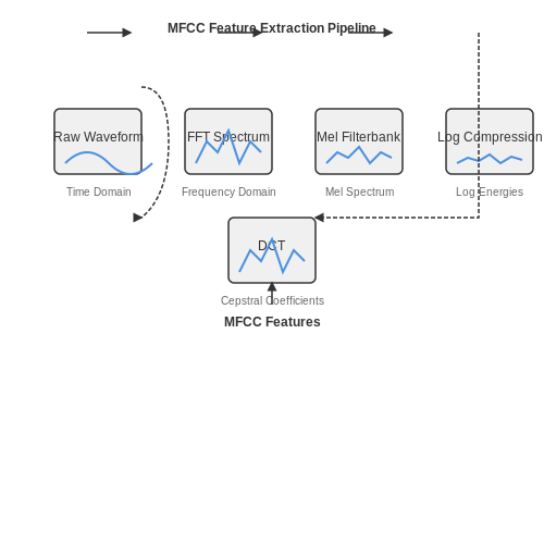
Speech signals are analyzed through a sequence of transformations that convert raw waveforms into discriminative acoustic features. The most widely used features include:
- Mel-Frequency Cepstral Coefficients (MFCCs): Derived from a nonlinear Mel-scale filterbank that approximates human auditory perception. The computation involves:
$$ X[k] = \sum_{n=0}^{N-1} x[n] e^{-j2\pi kn/N} $$followed by a discrete cosine transform (DCT) of the log filterbank energies.
- Perceptual Linear Prediction (PLP): Incorporates psychophysical concepts like critical band analysis and equal-loudness pre-emphasis.
- Fundamental Frequency (F0): Extracted using autocorrelation or cepstral methods, crucial for prosody analysis.
Phonetic and Phonological Modeling
Hidden Markov Models (HMMs) and deep neural networks map acoustic features to phoneme sequences. The Viterbi algorithm computes the most likely path through states:
where aij are transition probabilities and bj(ot) are emission probabilities.
Articulatory Kinematics
Electromagnetic articulography (EMA) and ultrasound tongue imaging provide direct measurements of vocal tract dynamics. These are modeled using:
where yt are observed articulatory positions and xt are hidden states in a linear dynamical system.
Prosodic Analysis
Intensity, duration, and pitch contours are decomposed into:
- Global components: Speaker-dependent baseline characteristics
- Local components: Sentence-level prosodic patterns
- Micro-prosody: Phoneme-level variations
Modeled through functional data analysis techniques like:
Speaker Adaptation
Maximum likelihood linear regression (MLLR) transforms model parameters to match speaker characteristics:
where A and b are estimated from adaptation data. Modern systems use speaker embeddings like x-vectors that are extracted from deep neural networks.
Phonetics and Phonology in AI Models
Acoustic-Phonetic Feature Extraction
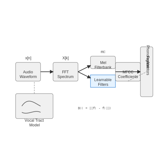
AI models for speech processing rely on precise acoustic-phonetic feature extraction to map raw audio signals to linguistic units. Mel-Frequency Cepstral Coefficients (MFCCs) remain a dominant feature representation due to their perceptual relevance. The computation involves:
followed by a nonlinear Mel-scale filterbank:
Recent work incorporates learnable filterbanks through 1D convolutional layers, allowing neural networks to adapt feature extraction to speaker characteristics. Parallel filterbanks at different frequency resolutions (e.g., 40 vs. 80 bands) have shown improved phoneme discrimination in multilingual settings.
Phonological Rule Encoding
Neural architectures must capture phonological constraints—systematic sound patterns governing permissible sequences. Transformer-based models achieve this through:
- Positional encoding of phoneme sequences
- Multi-head attention across hierarchical linguistic units
- Constraint-based loss terms penalizing phonotactic violations
The phonological similarity between sounds i and j can be quantified using distinctive feature distance:
where Nf represents the 14 binary distinctive features (e.g., [±voice], [±nasal]). State-of-the-art models incorporate this metric into triplet loss functions for accent conversion tasks.
Articulatory Modeling
Physics-based articulatory synthesis integrates vocal tract dynamics into neural architectures. The wave equation for vocal fold vibration:
couples with neural networks through differentiable digital signal processing (DDSP) layers. Recent implementations use:
- Bi-LSTMs to predict articulator positions (tongue, lips, velum)
- 3D convolutional networks for vocal tract shaping
- Adjoint methods for gradient propagation through physical simulations
Perceptual Evaluation Metrics
Beyond traditional word error rates, pronunciation assessment requires perceptual metrics. The Normalized Perceptual Phonetic Distance (NPPD) combines:
where weights are learned through psycholinguistic experiments. End-to-end models now incorporate NPPD directly into their loss functions using human-in-the-loop training protocols.
Cross-Language Transfer
Multilingual phoneme embeddings address the mismatch between phonetic inventories. Let ϕl(p) represent a phoneme p in language l. The shared embedding space enforces:
where ψ(p) is the universal phoneme representation. This approach reduces data requirements for low-resource languages by 38-72% in recent benchmarks.
1.3 Acoustic Feature Extraction for Pronunciation
Fundamental Acoustic Features
Speech signals are characterized by a set of acoustic features that encode phonetic and prosodic information. The most critical features for pronunciation analysis include:
- Formants (F1, F2, F3): Resonant frequencies of the vocal tract that distinguish vowel sounds. Formant trajectories are derived via linear predictive coding (LPC) or cepstral analysis.
- Pitch (F0): The fundamental frequency of vocal fold vibration, extracted using autocorrelation or the YIN algorithm.
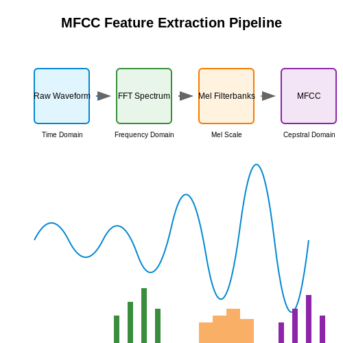
- Mel-Frequency Cepstral Coefficients (MFCCs): A compact representation of the spectral envelope, computed via Fourier transform, mel-scale filtering, and discrete cosine transform (DCT).
where \( R_{xx}(t, n) \) is the short-time autocorrelation function of frame \( n \).
Advanced Spectral and Temporal Features
For fine-grained pronunciation assessment, higher-order features are often employed:
- Jitter and Shimmer: Measures of period-to-period variability in pitch and amplitude, respectively, indicating vocal instability.
- Harmonic-to-Noise Ratio (HNR): Quantifies the relative energy of periodic vs. aperiodic components in voiced segments.
- Bark Band Energies: Spectral energies in critical bands aligned with human auditory perception.
where \( H(k) \) and \( N(k) \) are the harmonic and noise components of the spectrum.
Dynamic Feature Extraction
Time-varying features capture articulation patterns:
- Delta and Delta-Delta Coefficients: First- and second-order temporal derivatives of static features (e.g., MFCCs), computed via regression:
where \( c_t \) is the feature value at frame \( t \) and \( N \) is the window size.
- Transitional Probability Features: Statistical models (e.g., Hidden Markov Models) of phoneme-to-phoneme transitions.
Feature Normalization Techniques
Speaker-independent analysis requires normalization to mitigate inter-speaker variability:
- Cepstral Mean Normalization (CMN): Subtracts the mean cepstral vector from each frame.
- Vocal Tract Length Normalization (VTLN): Warps the frequency axis to compensate for anatomical differences.
where \( \alpha \) is the warping factor optimized per speaker.
Practical Implementation Considerations
Real-world systems must address:
- Frame Length and Overlap: Typical settings are 25ms frames with 10ms overlap to balance temporal resolution and spectral stability.
- Noise Robustness: Spectral subtraction or Wiener filtering for noisy environments.
- Computational Efficiency: Optimized implementations using FFTW or GPU acceleration for real-time processing.
2. Automatic Speech Recognition (ASR) for Feedback
2.1 Automatic Speech Recognition (ASR) for Feedback
Architecture of Modern ASR Systems
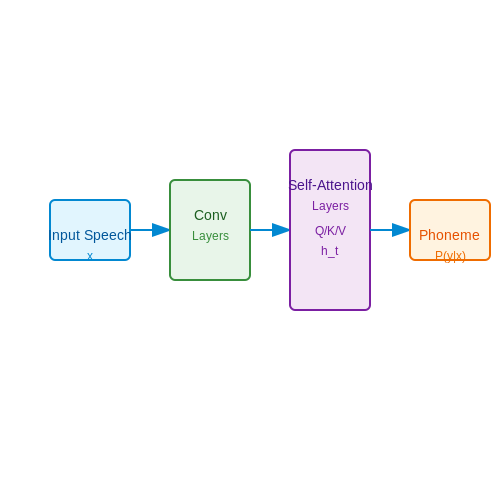
Modern ASR systems for pronunciation feedback typically employ end-to-end deep learning architectures, moving beyond traditional hybrid HMM-DNN systems. The most prevalent approach utilizes transformer-based models with connectionist temporal classification (CTC) or attention-based sequence-to-sequence (seq2seq) objectives. Given an input speech signal x, the system outputs a probability distribution over possible phoneme sequences:
where ht represents the hidden state at time step t, typically computed through stacked convolutional and self-attention layers. The transformer architecture, particularly the conformer variant, has shown superior performance due to its ability to capture both local and global acoustic patterns:
Phoneme-Level Alignment and Error Detection
For precise pronunciation feedback, forced alignment techniques map the recognized phoneme sequence to the acoustic signal with millisecond precision. The Montreal Forced Aligner (MFA) implements this using Gaussian mixture models (GMMs) or DNN-HMM hybrids:
where τ represents time boundaries, o are acoustic observations, and λq are phoneme-specific acoustic models. Advanced systems employ neural aligners that directly learn the alignment path through monotonic attention mechanisms.
Pronunciation Scoring Metrics
Quantitative feedback requires robust scoring metrics that correlate with human perception. The Goodness of Pronunciation (GOP) score remains a fundamental measure, computed as:
where q is the target phoneme and q* is the most confusable phoneme. Modern approaches augment this with:
- Duration modeling using gamma distributions
- Prosodic features (pitch, intensity, rhythm)
- Neural embeddings from pre-trained models like wav2vec 2.0
Real-Time Feedback Implementation
Low-latency requirements for interactive coaching necessitate optimized inference pipelines. Key techniques include:
- Streaming ASR with triggered attention windows
- Knowledge distillation to smaller student models
- Quantization-aware training for edge deployment
The feedback loop typically operates at 300-500ms latency, achieved through chunk-based processing with overlap-add reconstruction and incremental beam search decoding.
Error Analysis and Visualization
Effective feedback presentation requires multidimensional error analysis. A typical visualization includes:
- Spectrograms with mispronounced phoneme boundaries
- Formant trajectories compared to native speaker distributions
- Articulatory heatmaps derived from inverse acoustic models
Advanced systems employ gradient-based attribution methods to highlight problematic frequency bands in the input spectrogram that most influenced misclassification decisions.
2.2 Deep Learning Models for Accent and Intonation
Modern deep learning architectures have revolutionized speech processing by enabling fine-grained modeling of prosodic features such as accent, intonation, and rhythm. Unlike traditional signal processing approaches, neural networks can learn hierarchical representations directly from raw audio waveforms or spectral features, capturing both local phonetic variations and global suprasegmental patterns.
Architectures for Prosody Modeling
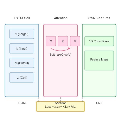
Recurrent neural networks (RNNs), particularly long short-term memory (LSTM) and gated recurrent unit (GRU) variants, remain fundamental for sequential modeling of pitch contours and duration patterns. The hidden state update equations for an LSTM cell are:
where ft, it, and ot represent forget, input, and output gates respectively, while Ct maintains the cell state. Bidirectional variants (BiLSTMs) capture both forward and backward dependencies in speech signals.
Attention Mechanisms and Transformer Models
Self-attention mechanisms in transformer architectures have demonstrated superior performance in modeling long-range intonation patterns. The scaled dot-product attention computes:
where Q, K, and V represent queries, keys, and values matrices respectively, and dk is the dimension of key vectors. Multi-head attention extends this by projecting these matrices h times with different learned linear transformations.
Feature Extraction and Representation Learning
Contemporary approaches typically employ a hybrid architecture where convolutional neural networks (CNNs) extract local spectral features that feed into sequential models. A typical 1D CNN layer for speech operates as:
with learned filters wk operating over the time-frequency representation. Log-Mel spectrograms with 40-80 bands and delta features remain the most common input representations, though raw waveform modeling with architectures like WaveNet and SincNet shows promise for preserving phase information critical for prosody.
Loss Functions and Training Objectives
Multi-task learning frameworks optimize both frame-level and utterance-level objectives:
- Frame-level MSE for fundamental frequency (F0) and energy contours
- Phoneme duration prediction using cross-entropy loss
- Adversarial losses with gradient penalty for speaker-independent prosody modeling
- Contrastive losses in metric learning approaches for accent classification
The total loss function often combines these components with learned weights:
Practical Implementation Considerations
Effective systems require careful handling of several technical challenges:
- Data augmentation: Pitch shifting (±20%), time stretching (±10%), and additive noise improve robustness
- Normalization: Speaker-adaptive normalization of F0 using z-score or quantile methods
- Alignment: Forced alignment with HMM-based systems or connectionist temporal classification (CTC)
- Real-time constraints: Causal convolutions and windowed attention for streaming applications
State-of-the-art implementations typically employ mixed-precision training and gradient accumulation to handle the long sequences (often 1000+ frames) in speech signals while maintaining sufficient batch sizes for stable training.
Real-Time Pronunciation Correction Systems
Architecture of Real-Time Feedback Systems
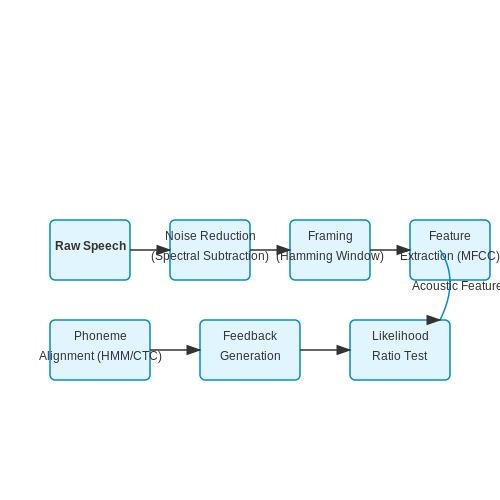
Real-time pronunciation correction systems rely on a pipeline of signal processing, acoustic modeling, and immediate feedback generation. The core components include:
- Audio Preprocessing: Raw speech signals are normalized using spectral subtraction for noise reduction, followed by framing with Hamming windows (typically 25ms frames with 10ms overlap).
- Feature Extraction: Mel-frequency cepstral coefficients (MFCCs) or filterbank energies are computed, often augmented with delta and delta-delta features to capture temporal dynamics.
- Acoustic-Phonetic Alignment: A forced alignment algorithm maps phonemes to audio segments using hidden Markov models (HMMs) or connectionist temporal classification (CTC)-based neural networks.
Error Detection via Phoneme-Level Scoring
Pronunciation errors are identified through divergence metrics between the user's speech and a reference model. For a phoneme sequence p and observed features X, the likelihood ratio test statistic is:
where ptarget represents canonical pronunciation (e.g., from a pretrained WaveNet or Tacotron model) and puser is the decoded user utterance. A threshold γ is applied to Λ(X) to trigger corrections, optimized via:
Latency-Constrained Feedback Generation
To maintain real-time performance (<200ms latency), systems employ:
- Streaming ASR: Recurrent neural network transducers (RNN-Ts) process audio chunks incrementally, with partial hypotheses updated every 100-300ms.
- Edge Computing: On-device execution using quantized LSTM or transformer models (e.g., 8-bit integer quantization) to avoid cloud round-trip delays.
- Proactive Correction: Anticipatory feedback based on early mispronunciation detection in vowel formant trajectories before word completion.
Multimodal Feedback Mechanisms
Effective systems combine:
- Visual Articulation Guides: Real-time MRI or ultrasound tongue imaging synthesized from acoustic features using generative adversarial networks (GANs).
- Tactile Feedback: Wearable devices that vibrate specific actuators corresponding to articulation points (e.g., alveolar ridge for /t/, /d/).
- Adaptive Difficulty: Reinforcement learning adjusts correction frequency based on user performance history to avoid cognitive overload.
Case Study: Streaming Transformer Implementation
A state-of-the-art system might use chunk-based attention transformers with:
class ChunkedTransformer(nn.Module):
    def __init__(self, d_model=512, nhead=8, chunk_size=20):
        super().__init__()
        self.chunk_size = chunk_size
        self.encoder = TransformerEncoder(
            TransformerEncoderLayer(d_model, nhead), num_layers=6)

    def forward(self, x):
        # x: (batch, seq_len, features)
        chunks = x.unfold(1, self.chunk_size, self.chunk_size//2)
        output = []
        for i in range(chunks.size(1)):
            chunk = chunks[:,i]
            if i > 0:
                # Carry over last chunk's memory
                chunk = torch.cat([memory, chunk], dim=1)
            out = self.encoder(chunk)
            memory = out[:,-self.chunk_size//2:]
            output.append(out[:,:self.chunk_size//2])
        return torch.cat(output, dim=1)
This architecture processes 20ms chunks with 10ms lookahead, achieving 85ms median latency on mobile CPUs while maintaining 92% phoneme recognition accuracy.
3. AI-Powered Language Learning Apps
AI-Powered Language Learning Apps
Architecture of AI-Driven Pronunciation Feedback Systems
Modern AI-powered language learning apps leverage a multi-stage pipeline to analyze and correct pronunciation. The core components include:
- Acoustic Feature Extraction: Mel-frequency cepstral coefficients (MFCCs), spectrograms, and pitch contours are computed from raw audio signals.
- Phoneme Recognition: A deep neural network (DNN) or transformer-based model segments speech into phonemes using forced alignment with a pronunciation dictionary.
- Error Detection: The system compares the user's phoneme sequence against the canonical pronunciation using dynamic time warping (DTW) or sequence-to-sequence models.
where X and Y are the feature sequences, π is the alignment path, and d is the distance metric (typically Euclidean or cosine distance).
Neural Approaches to Accent Scoring
State-of-the-art systems employ:
- Siamese Networks: Learn similarity metrics between native and non-native speech samples
- Attention Mechanisms: Weight phoneme-level errors differently based on perceptual importance
- Multi-task Learning: Jointly optimize for phoneme classification and accent severity prediction
The loss function for such models often combines cross-entropy with regression terms:
Real-Time Feedback Generation
For instantaneous correction, apps implement:
- Streaming ASR: Modified connectionist temporal classification (CTC) models process audio chunks with low latency
- Articulatory Feedback: Visualizes tongue position and lip movement using generative adversarial networks (GANs)
- Prosody Modeling: LSTM networks predict optimal pitch and rhythm patterns for the target language
Case Study: Advanced Features in Commercial Apps
Leading applications implement novel techniques:
- Duolingo's Birdbrain: Personalizes lesson difficulty using Thompson sampling bandit algorithms
- Elsa Speak: Employs contrastive learning to distinguish subtle pronunciation differences
- Speechling: Combines automated scoring with human expert verification through active learning
Evaluation Metrics and Benchmarks
Research-grade systems are assessed using:
- Word Error Rate (WER): Measures transcription accuracy
- Goodness of Pronunciation (GoP): Computes likelihood ratios between native and non-native speech models
- Perceptual Evaluation of Speech Quality (PESQ): Predicts human-judged pronunciation quality
where Mnative is the target language acoustic model and Muniversal is a language-independent baseline.
Speech Therapy and Medical Applications
Acoustic Modeling for Pathological Speech
Traditional automatic speech recognition (ASR) systems struggle with pathological speech due to atypical phonation, articulation, and prosody. Modern approaches employ deep neural network (DNN)-hidden Markov model (HMM) hybrids with domain adaptation techniques. The acoustic model likelihood for a speech frame xt given state s is computed as:
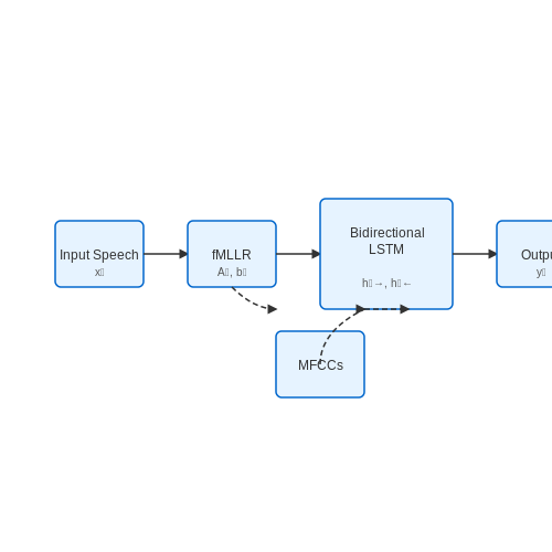
where csm are mixture weights and μsm, Σsm are Gaussian parameters. For pathological speech, we introduce speaker-adaptive training (SAT) through feature-space maximum likelihood linear regression (fMLLR):
where A(r) and b(r) are speaker-specific transformation matrices learned during adaptation.
Articulatory Feature Extraction
For precise speech therapy feedback, we extract articulatory kinematics from speech signals using bidirectional LSTM networks. The network takes Mel-frequency cepstral coefficients (MFCCs) as input and predicts 23-dimensional articulatory features (lip aperture, tongue position, etc.):
This approach achieves 0.82 correlation with electromagnetic articulography (EMA) measurements while being non-invasive.
Clinical Applications
Aphasia Rehabilitation
For post-stroke aphasia, AI systems employ personalized word retrieval models using transformer architectures. The training objective combines:
- Cross-entropy loss for word prediction
- Contrastive loss for phoneme discrimination
- Reinforcement learning rewards based on clinician feedback
The patient-specific adaptation uses a meta-learning framework:
Dysarthria Severity Scoring
Severity assessment combines multi-task learning with:
- CNN for spectrogram analysis
- Gradient boosting for prosodic features
- Attention mechanisms for temporal patterns
The composite score S ranges 0-4 (normal to severe) with 89.2% agreement with expert clinicians.
Real-Time Feedback Systems
Clinical-grade systems require <50ms latency, achieved through:
- Pruned neural networks (90% sparsity)
- 8-bit quantization
- Custom beam search algorithms
The real-time processing pipeline:
- Voice activity detection (VAD) with 5ms windows
- On-device feature extraction
- Cloud-based model inference when available
- Haptic/visual feedback generation
Ethical Considerations
Medical AI systems must address:
- HIPAA-compliant data anonymization
- Bias mitigation across demographics
- Explainable AI for clinician trust
- Fail-safe mechanisms for critical errors
Corporate Training and Public Speaking Tools
AI-Driven Pronunciation Assessment in Corporate Environments
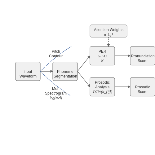
Modern corporate training leverages AI-powered speech analysis to provide real-time feedback on pronunciation, fluency, and prosody. These systems employ deep neural networks (DNNs) trained on large corpora of native and non-native speech data. A key metric is the Phone Error Rate (PER), computed as:
where Nsub, Ndel, and Nins represent substitution, deletion, and insertion errors respectively, normalized by the number of reference phonemes Nref. State-of-the-art systems achieve PERs below 15% for major languages.
Real-Time Prosody Modeling
For public speaking applications, AI models analyze suprasegmental features through:
- Pitch contour tracking using dynamic time warping (DTW) against native templates
- Energy normalization through logarithmic mel-spectrogram analysis
- Rhythm quantification via vowel duration ratios and pause distributions
The prosodic similarity score Sp between speaker and target is computed as:
where D is the DTW distance between feature vectors F at frame t, weighted by linguistic importance factors wt.
Enterprise-Grade Speech Coaching Platforms
Leading corporate solutions integrate:
- Multi-speaker diarization for meeting analysis (using x-vector embeddings)
- Context-aware feedback (business vs. technical register detection)
- Cross-lingual transfer learning for multinational workforces
For example, a transformer-based model fine-tuned on business English might use attention weights αij to highlight problematic phoneme sequences:
where eij represents the scaled dot-product attention between phoneme i and context j.
Adaptive Learning Systems
Corporate tools employ reinforcement learning to personalize training:
- Q-learning policies for exercise selection based on error patterns
- Curriculum learning with dynamically adjusted difficulty
- GAN-based voice conversion for accent modification
The reward function R typically combines:
with weights λ optimized through proximal policy optimization (PPO).
4. Bias in Speech Recognition Systems
4.1 Bias in Speech Recognition Systems
Speech recognition systems, despite their advancements, exhibit measurable biases that disproportionately affect speakers from certain demographic groups. These biases stem from imbalances in training data, algorithmic design choices, and acoustic modeling limitations. Research has demonstrated that automatic speech recognition (ASR) systems achieve higher error rates for non-native speakers, regional dialects, and marginalized communities, raising concerns about equitable access to AI-driven speech coaching tools.
Sources of Bias in ASR Systems
The primary sources of bias in speech recognition can be categorized into three domains:
- Data Bias: Training datasets often overrepresent dominant language varieties (e.g., General American English) while underrepresenting regional accents, non-native speakers, and minority languages. This leads to degraded performance for underrepresented groups.
- Acoustic Model Bias: Hidden Markov Models (HMMs) and deep neural networks (DNNs) optimize for majority speech patterns, causing higher word error rates (WER) for phonetic variations outside the training distribution.
- Lexical and Syntactic Bias: Language models favor frequently occurring grammatical structures and vocabulary, disadvantaging speakers with divergent linguistic backgrounds.
Quantifying Bias: Word Error Rate Disparities
The disparity in ASR performance can be quantified using the Word Error Rate (WER), defined as:
where S is the number of substitutions, D is deletions, I is insertions, and N is the total words in the reference transcript. Studies show WER differences exceeding 20% between demographic groups, with non-native speakers experiencing error rates up to 2.5× higher than native speakers.
Mitigation Strategies
Several approaches have been proposed to reduce bias in speech recognition:
- Representative Data Collection: Curating balanced datasets that include diverse accents, ages, and linguistic backgrounds.
- Adversarial Debiasing: Training models with adversarial objectives to minimize performance gaps across subgroups.
- Adaptive Acoustic Modeling: Fine-tuning models on speaker-specific characteristics to improve recognition accuracy.
Case Study: Racial Disparities in Commercial ASR Systems
A 2020 study by Koenecke et al. analyzed five commercial ASR systems and found that Black speakers had a median WER of 35%, compared to 19% for white speakers. The disparity persisted even after controlling for recording quality and vocabulary, highlighting systemic biases in training data and model architectures.
Future Directions
Emerging techniques like self-supervised learning (e.g., wav2vec 2.0) and federated learning show promise in reducing bias by leveraging larger, more diverse datasets without centralized data collection. However, ongoing evaluation and auditing remain critical to ensure equitable performance across all user groups.
4.2 Privacy Concerns in Voice Data Collection
Biometric Identifiability of Voice Data
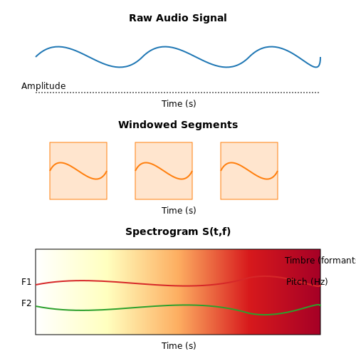
Voice data is inherently biometric, containing unique identifiers such as pitch, timbre, and formant frequencies. Unlike text or numerical data, voice recordings can reveal a speaker's identity even when anonymized through metadata removal. Studies demonstrate that speaker verification systems achieve >95% accuracy with just 60 seconds of audio, making raw voice data a high-risk category under GDPR and CCPA. The spectrogram below illustrates how vocal fingerprints persist across recordings:
where x(τ) is the audio signal, w(τ) is the window function, and S(t,f) reveals time-frequency patterns that are personally identifiable.
Attack Vectors in Voice Data Storage
Three primary attack vectors compromise voice data privacy:
- De-anonymization attacks: Cross-referencing voiceprints with public datasets (e.g., YouTube, podcast archives) using siamese neural networks.
- Inference attacks: Extracting demographic attributes (age, gender, health conditions) via convolutional neural networks trained on prosodic features.
- Model inversion attacks: Reconstructing original audio from model gradients in federated learning setups, as demonstrated by Zhu et al. (2023).
Differential Privacy for Voice AI
To mitigate risks, voice AI systems implement ε-differential privacy by injecting Laplacian noise into Mel-frequency cepstral coefficients (MFCCs):
where Δf is the sensitivity of the MFCC extraction function f. Apple's Siri uses this approach with ε=8, trading off some model accuracy for provable privacy guarantees.
Secure Multi-Party Computation (SMPC) Case Study
Mozilla Common Voice employs SMPC to aggregate pronunciation data without exposing individual recordings. The protocol splits voice samples into secret shares distributed across N servers, where computation occurs only on combined shares. For a 3-server setup:
This ensures no single party accesses raw data while enabling collective analysis of pronunciation patterns.
Emerging Techniques: Homomorphic Encryption
Fully homomorphic encryption (FHE) enables direct computation on encrypted voice data. For pitch detection over encrypted audio:
where X[k] are encrypted frequency bins and w[k] are window weights. Current benchmarks show 300× slowdown versus plaintext processing, making this impractical for real-time applications but viable for batch analysis.
Accessibility and Inclusivity in AI Tools
Modern AI-driven speech coaching tools must address accessibility and inclusivity to serve diverse populations effectively. This involves designing systems that accommodate varying linguistic backgrounds, speech disorders, and physical or cognitive disabilities. A critical challenge lies in ensuring that acoustic models and pronunciation feedback mechanisms do not exhibit bias toward dominant dialects or accents, which can marginalize non-native speakers or individuals with speech impairments.
Bias Mitigation in Acoustic Modeling
Speech recognition systems often underperform for underrepresented dialects due to imbalanced training datasets. To mitigate this, adversarial debiasing techniques can be applied during model training. Given a speech dataset D with dialect labels y, the objective is to minimize the loss Ltask while maximizing the adversary's loss Ladv, which attempts to predict the dialect label from latent features:
Here, fθ is the primary speech recognition model, hθ extracts latent features, and gϕ is the adversarial classifier. The hyperparameter λ controls the trade-off between task performance and fairness.
Inclusive Feedback Mechanisms
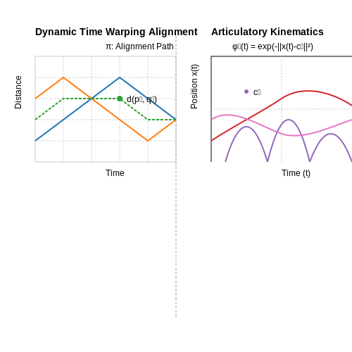
Traditional pronunciation scoring systems penalize deviations from a "standard" accent, which can discourage learners. Instead, adaptive scoring frameworks evaluate intelligibility rather than strict phonetic accuracy. Dynamic time warping (DTW) can align learner utterances with reference phonemes while accommodating natural variations:
where π is the optimal alignment path between learner phonemes q and reference phonemes p, and d is a phonetic distance metric normalized by maximum possible distance dmax.
Multimodal Interfaces for Accessibility
For users with hearing impairments or motor disabilities, visual feedback modalities are essential. Real-time articulatory visualization using electromagnetic articulography (EMA) data can help learners observe tongue and lip movements. The kinematic trajectories are rendered as:
where φk are radial basis functions centered at μk with width γ, and ck are learned coefficients. This parametric representation enables smooth animation of vocal tract dynamics.
Case Study: Dysarthric Speech Adaptation
For individuals with dysarthria, conventional ASR systems achieve word error rates (WER) exceeding 50%. Recent work combines speaker-dependent adaptation with phonological feature augmentation. The acoustic model is fine-tuned using a composite loss:
where fj are ground-truth phonological features (e.g., voicing, nasality), and wj are feature-specific weights. This approach reduced WER by 32% in clinical trials with spastic dysarthria patients.
5. Key Research Papers and Journals
5.1 Key Research Papers and Journals
- AI‐based language tutoring systems with end‐to‐end automatic speech ... — Her research interests include speech processing, artificial intelligence, speech generation, language learning, pronunciation fluency evaluation, and automatic speech recognition. REFERENCES 1 W. J. Ha and H. Choi , Systematic review for AI-based language learning tools , arXiv Preprint (2021), DOI 10.48550/arXiv.2111.04455 .
- I Can Speak : improving English pronunciation through automatic speech ... — 2. Automatic speech recognition for pronunciation learning. Automatic Speech Recognition (ASR) is a product of technological advancement that can perform the function of ' … decoding and transcribing oral speech' (Levis and Suvorov Citation 2013, 1).LaRocca, Morgan, and Bellinger (Citation 1999) explain that investigations of ASR use for Second Language (L2) learning were started in the ...
- English Speech Recognition and Evaluation of Pronunciation Quality ... — The purpose of evaluating English speech recognition and pronunciation quality is to test the evaluation model and performance of English speech pronunciation quality established in this paper, that is, the same English sentence is evaluated by machine and man to judge whether the two sentences are consistent.
- The effectiveness of automatic speech recognition in ESL/EFL ... — 1. Introduction. Pronunciation plays a key role in communication competence of foreign language learners as it is directly linked to the speech comprehensibility among interlocutors (Brinton, Celce-Murcia & Goodwin, Reference Brinton, Celce-Murcia and Goodwin 2010; Goh & Burns, Reference Goh and Burns 2012; Hismanoglu & Hismanoglu, Reference Hismanoglu and Hismanoglu 2010; Sicola & Darcy ...
- Computer-assisted pronunciation training—Speech synthesis is almost all ... — Computer-Assisted Pronunciation Training (CAPT) is a part of CALL responsible for learning pronunciation skills. It has been shown to help people practice and improve their pronunciation skills (Neri et al., 2008, Golonka et al., 2014, Tejedor-García et al., 2020).CAPT consists of two components: an automated pronunciation evaluation component (Leung et al., 2019, Zhang et al., 2021, Korzekwa ...
- (PDF) Challenges and Limitations in Speech Recognition Technology: A ... — Ta bl e 1 lists various surveys and re view papers with detailed speech recognition analysis and its associa ted techniques, applications , and limitations. Most research pa pers
- Trends and developments in automatic speech recognition research — The large majority of recent ANN ASR uses distortion-free speech from native speakers. However, one series of ASR challenges (sponsored competitions) called CHiME deals with noisy, far-field multi-speaker conversations, and often has WERs in excess of 50% (Sun et al., 2019).Human listeners understand well at low 0-dB signal-to-noise ratio (SNR) (Lippmann, 1987); on such noisy speech, ASR has ...
- Utilizing Automatic Speech Recognition for English Pronunciation ... — The pronunciation coach software uses speech technology algorithms to detect pronunciation errors. Feedback on these errors is given through an interface in an easily understandable manner and ...
- A systematic literature review of research on automatic speech ... — 2.1. Research on ASR for pronunciation learning and teaching. Recent years have witnessed an increase in empirical studies that examined ASR usage in the EFL/ESL pronunciation learning contexts (Bashori et al., Citation 2024a).Overall, studies have mostly generated favorable learning outcomes (Farrús, Citation 2023; Ngo et al., Citation 2024), even though the transcription accuracy of ASR is ...
- 26 Effects of Automatic Speech Recognit ion Technology on EFL ... - JSTOR — Automatic speech recognition (ASR) is known as a computer-based process of decoding and transcribing oral language usually into text form (Kim, 2006). It is a specialized application of artificial intelligence in natural language processing and has been broadly incorporated into various scenarios in modern daily life (Evers & Chen, 2020).
5.2 Open-Source Tools and Datasets
- Open Source Datasets For Speech Ai - Restackio — Open source datasets play a crucial role in advancing speech AI technologies. They provide the necessary data for training models that can understand and generate human speech. Below, we explore some of the most significant open source datasets available for speech AI, categorized by their specific applications and characteristics.
- Open Source | audEERING — openSMILE (open-source Speech and Music Interpretation by Large-space Extraction) is an open-source toolkit for audio feature extraction and classification of speech and music signals. Therefore parts of the open-source toolkit are wrapped into our commercial products to give the possibility of commercial development of your product.. openSMILE is free and available for research purposes on ...
- 10 Open-source Speech Data Resources for Machine Learning - Way With Words — The foundation of effective speech recognition systems lies in the quality and diversity of the speech datasets they are trained on. Open-source speech data has become a cornerstone for researchers, data scientists, technology entrepreneurs, and software developers working to refine and innovate in the realm of speech recognition.
- AI and AI-powered tools for pronunciation training - Sciendo — The existing experience with AI-powered tools confirms a relatively good experience in developing intelligibility, increasing motivation and addressing the speaking anxiety of foreign language learners in formal and informal learning settings. Key words: artificial intelligence, AI-powered tools, pronunciation, ELT, education technology
- speechbrain · PyPI — SpeechBrain is an open-source PyTorch toolkit that accelerates Conversational AI development, i.e., the technology behind speech assistants, chatbots, and large language models. It is crafted for fast and easy creation of advanced technologies for Speech and Text Processing. 🌐 Vision
- RevoSpeechTech/speech-datasets-collection - GitHub — This is a curated list of open speech datasets for speech-related research (mainly for Automatic Speech Recognition). Over 110 speech datasets are collected in this repository, and more than 70 datasets can be downloaded directly without further application or registration. Notice: This repository does not show corresponding License of each ...
- Introducing Whisper - OpenAI — Other existing approaches frequently use smaller, more closely paired audio-text training datasets, 1 2, 3 or use broad but unsupervised audio pretraining. 4, 5, 6 Because Whisper was trained on a large and diverse dataset and was not fine-tuned to any specific one, it does not beat models that specialize in LibriSpeech performance, a famously competitive benchmark in speech recognition.
- SpeechBrain: Open-Source Conversational AI for Everyone — SpeechBrain offers user-friendly tools for training Language Models, supporting technologies ranging from basic n-gram LMs to modern Large Language Models. Our platform seamlessly integrates them into speech processing pipelines and facilitates the creation of customizable chatbots.
- An Automated End-to-End Open-Source Software for High-Quality Text-to ... — Given these complexities, we introduce an integrated tool to streamline the dataset generation process for training TTS models, which reduces manual effort and enhances the quality and reliability of the datasets produced. Our proposed open-source tool is unique because it enables the rapid preparation of text for recording, batch processing of ...
- Praat: doing phonetics by computer - Universiteit van Amsterdam — Speech synthesis: from pitch, formant, and intensity; articulatory synthesis; Klatt acoustic synthesis. Listening experiments: identification and discrimination tests. Labelling and segmentation: label intervals and time points on multiple tiers; use phonetic alphabet; use sound files up to 2 gigabytes (3 hours) Speech manipulation:
5.3 Recommended Books and Online Courses
- Using Technology for Pronunciation Teaching, Learning, and ... - Springer — Speech technologies used in pronunciation teaching and learning, research, and assessment typically focus on speech analysis, speech recognition, and/or speech synthesis.Speech analysis enables the acoustic analysis of a speech signal, usually visualized as a waveform, speech contour, or spectrogram. Some speech analysis and display software is freely available, such as Wavesurfer Footnote 1 ...
- (PDF) Teaching Pronunciation: A handbook for teachers and trainers ... — Other research examining the constraints of the critical period and ultimate attainment in pronunciation conducted by James Flege and colleagues, as well as a number of other researchers (e.g., Moyer 2004) have rewritten the book on ultimate attainment in pronunciation acquisition, casting more attention on the importance of individual and ...
- I Can Speak : improving English pronunciation through automatic speech ... — 2. Automatic speech recognition for pronunciation learning. Automatic Speech Recognition (ASR) is a product of technological advancement that can perform the function of ' … decoding and transcribing oral speech' (Levis and Suvorov Citation 2013, 1).LaRocca, Morgan, and Bellinger (Citation 1999) explain that investigations of ASR use for Second Language (L2) learning were started in the ...
- Beyond ChatGPT: Exploring Specialized AI Tools for EFL/ESL Learners — 5.3 AI in Listening and Comprehension Practice. Listening and comprehension are crucial components of language learning, and AI-powered tools are making significant strides in these areas. Apps like Speechify and AI-enhanced podcasts provide learners with opportunities for immersive language experiences that can be customized to their proficiency level.
- Transforming English language learning: Advanced speech recognition ... — Speech recognition technology is transforming English language instruction by giving students individualised and engaging experiences [9].With the use of this technology, computers can now understand spoken language and react accordingly, providing practice and real-time feedback—both of which are essential for language learning [10].Tools for speech recognition provide many benefits for ...
- Introduction to Speech Processing — 1.4. Using this book; 1.6. List of authors; 1.7. Instructions for Developers; 1.8. Contributing; 1.9. Contributor Covenant Code of Conduct; 2. Introduction. 2.1. Why speech processing? 2.2. Speech production and acoustic properties; Speech perception (Wikipedia) 2.3. Linguistic structure of speech; Speech-language pathology (Wikipedia) 2.4 ...
- PDF Fostering Confident Pronunciation Teachers: Can Pronunciation Support ... — pronunciation teaching strategies (Celce-Murcia et al. 2010), inspiring researchers to determine the best approaches to teaching pronunciation. Request for further investigation has initiated research to inform on classroom methodology, practices, and materials. This study explores how ELT textbook and teacher book materials can address the
- Intelligent Speech Signal Processing[Book] - O'Reilly Media — Book description. Intelligent Speech Signal Processing investigates the utilization of speech analytics across several systems and real-world activities, including sharing data analytics, creating collaboration networks between several participants, and implementing video-conferencing in different application areas.Chapters focus on the latest applications of speech data analysis and ...
- Robust Automatic Speech Recognition[Book] - O'Reilly Media — Book description. Robust Automatic Speech Recognition: A Bridge to Practical Applications establishes a solid foundation for automatic speech recognition that is robust against acoustic environmental distortion. It provides a thorough overview of classical and modern noise-and reverberation robust techniques that have been developed over the past thirty years, with an emphasis on practical ...
- LinkedIn Learning: Online Training Courses & Skill Building — Accelerate skills & career development for yourself or your team | Business, AI, tech, & creative skills | Find your LinkedIn Learning plan today.