Large Scale Pretraining for Vision-Language Models
1. Key Concepts and Definitions
Key Concepts and Definitions
Vision-Language Models (VLMs)
Vision-Language Models (VLMs) are a class of deep learning architectures designed to jointly process and understand both visual (image or video) and textual (natural language) data. These models learn a shared embedding space where semantically similar inputs from both modalities are mapped close together. The core objective is to enable tasks such as image captioning, visual question answering (VQA), and cross-modal retrieval by aligning visual and linguistic representations.
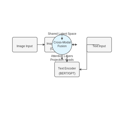
The foundational architecture of VLMs typically consists of:
- Image Encoder: A convolutional neural network (CNN) or Vision Transformer (ViT) that extracts hierarchical features from input images.
- Text Encoder: A transformer-based model (e.g., BERT, GPT) that processes tokenized text inputs.
- Cross-Modal Fusion: A mechanism (e.g., attention layers, projection heads) to align visual and textual embeddings in a shared latent space.
Pretraining Objectives
Large-scale pretraining for VLMs involves optimizing multiple self-supervised objectives to learn robust representations. Key pretraining objectives include:
where \( s(v_i, t_i) \) is the similarity score between image \( v_i \) and its paired text \( t_i \), \( au \) is a temperature parameter, and \( N \) is the batch size. This contrastive loss encourages paired samples to have higher similarity than unpaired ones.
Other common objectives include:
- Masked Language Modeling (MLM): Randomly masks tokens in the text and predicts them using surrounding context and visual features.
- Image-Text Matching (ITM): Classifies whether an image-text pair is matched or not.
- Region-Word Alignment: Aligns image regions with corresponding words using attention mechanisms.
Scaling Laws and Model Efficiency
The performance of VLMs follows scaling laws analogous to those observed in language models. Key parameters include:
where \( P \) is model performance, \( N \) is the number of parameters, \( D \) is dataset size, and \( \alpha, \beta \) are scaling exponents. Empirical studies show that increasing \( N \) and \( D \) monotonically improves performance, but with diminishing returns.
Efficiency considerations for large-scale pretraining include:
- Mixed-Precision Training: Uses FP16/FP32 hybrid precision to reduce memory usage.
- Gradient Checkpointing: Trade-offs memory for recomputation during backpropagation.
- Data Parallelism: Distributes batches across multiple GPUs to accelerate training.
Dataset Curation and Bias Mitigation
Large-scale pretraining relies on web-scraped datasets (e.g., LAION, Conceptual Captions), which introduce biases and noise. Mitigation strategies include:
- Filtering: Removing toxic or low-quality samples using CLIP-based similarity thresholds.
- Debiasing: Adversarial training or reweighting to reduce spurious correlations.
- Diversity Sampling: Ensures balanced representation across demographic and contextual attributes.
Recent work also employs synthetic data augmentation techniques, such as generating captions using LLMs or perturbing images with diffusion models, to improve coverage of rare concepts.
Architectures for Vision-Language Pretraining
Dual-Encoder Architectures
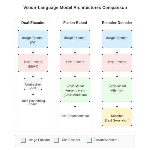
Dual-encoder architectures process vision and language inputs through separate encoders before fusing their representations. The image encoder, typically a Vision Transformer (ViT) or ResNet, maps input images to a latent space, while the text encoder, often a transformer like BERT, processes tokenized text. The similarity between modalities is computed via a contrastive loss, such as InfoNCE:
where s(vi, ti) measures cosine similarity between image and text embeddings, and τ is a temperature parameter. CLIP and ALIGN pioneered this approach, demonstrating scalability with web-scale noisy data.
Fusion-Based Architectures
Fusion architectures employ cross-modal attention to enable fine-grained interaction between vision and language representations. The image and text embeddings are concatenated and fed into a transformer that learns modality-agnostic features. Key variants include:
- Single-Stream: Early fusion (e.g., VisualBERT) processes concatenated image patches and text tokens through a shared transformer.
- Dual-Stream: Late fusion (e.g., ViLBERT) maintains separate encoders with cross-modal attention layers for intermediate fusion.
The attention mechanism computes:
where Q, K, V are derived from both modalities. This enables tasks like visual question answering by learning grounded representations.
Encoder-Decoder Architectures
Models like SimVLM and CoCa use a hybrid encoder-decoder approach. The encoder processes both modalities, while the decoder generates text autoregressively. The training objective combines contrastive loss and language modeling loss:
where λ1 and λ2 balance the objectives. This architecture excels at generative tasks like image captioning while retaining strong retrieval performance.
Scalability Considerations
Large-scale pretraining requires architectural optimizations:
- Gradient Checkpointing: Reduces memory by recomputing activations during backward passes.
- Mixed Precision Training: Uses FP16/FP32 hybrid precision to accelerate computation.
- Model Parallelism: Distributes layers across GPUs for models exceeding single-device memory.
Recent work like PaLI-3 demonstrates that scaling to billions of parameters with sparse expert mixtures (e.g., Switch Transformers) improves few-shot performance while maintaining training efficiency.
Common Pretraining Objectives
Contrastive Learning
Contrastive learning objectives train vision-language models to align paired image-text samples while pushing unpaired samples apart in a shared embedding space. The most widely used formulation is the InfoNCE loss:
where v and t are image and text embeddings, s(·,·) computes similarity (typically cosine), τ is a temperature parameter, and B is the batch of negative samples. CLIP and ALIGN demonstrated this approach's effectiveness at scale.
Masked Language Modeling
Adapted from BERT, masked language modeling (MLM) randomly masks text tokens and predicts them using surrounding context and paired visual features:
where M denotes masked token positions. Vision-language models like ViLBERT and LXMERT combine MLM with image region masking for cross-modal learning.
Image-Text Matching
This binary classification task predicts whether an image-text pair is matched (positive) or randomly paired (negative). The loss is typically formulated as:
where y ∈ {0,1} indicates match status and σ is the sigmoid function. Models like UNITER use hard negatives mined from contrastive learning to improve discrimination.
Prefix Language Modeling
Inspired by GPT, prefix LM processes text autoregressively conditioned on visual features. Given an image v and text tokens t1:n, the objective is:
This approach, used in models like SimVLM and CoCa, enables both understanding and generation capabilities.
Multimodal Fusion Objectives
Advanced models employ hybrid objectives combining multiple pretraining tasks. For example, ALBEF integrates contrastive learning, MLM, and ITM with a momentum encoder, while BEiT-3 unifies masked data modeling across modalities using a shared transformer.
The choice of objectives depends on the target capabilities - contrastive learning excels at retrieval, while autoregressive objectives better support generation tasks. State-of-the-art models often pretrain with 3-5 complementary objectives.
2. Large-Scale Datasets for Vision-Language Pretraining
Large-Scale Datasets for Vision-Language Pretraining
The efficacy of vision-language models (VLMs) hinges on the quality, diversity, and scale of the training datasets. Modern VLMs leverage multi-modal datasets that pair images with textual descriptions, enabling joint representation learning across modalities. Three critical dimensions define these datasets: size (number of samples), modality alignment (quality of image-text pairs), and domain coverage (breadth of visual and linguistic concepts).
Key Dataset Characteristics
Large-scale vision-language datasets typically exhibit the following properties:
- Cross-modal alignment: Each image is paired with one or more textual descriptions (captions, labels, or metadata). The strength of this pairing directly impacts model performance.
- Diverse domains: Datasets span natural scenes, specialized domains (medical, satellite), and synthetic data to ensure generalization.
- Noise robustness: Real-world datasets contain misaligned pairs, requiring preprocessing or noise-tolerant training techniques.
Notable Datasets
1. Conceptual Captions (CC)
Comprising 3.3M image-text pairs, CC was automatically collected from web pages, with alt-text serving as weak supervision. The dataset prioritizes scale over precise alignment, making it a testbed for noise-robust learning. Images are filtered for quality but retain web-scale diversity.
2. LAION-5B
At 5.85B CLIP-filtered pairs, LAION-5B is the largest publicly available dataset. It uses CLIP's embedding space to ensure cosine similarity between image and text embeddings exceeds a threshold (typically 0.28). The dataset enables training billion-parameter models but requires careful handling of biases and NSFW content.
3. COYO-700M
A curated subset of LAION, COYO-700M applies stricter filtering: deduplication, aesthetic scoring (>5.0), and text-length constraints. The balanced quality-quantity trade-off makes it suitable for mid-scale pretraining.
Dataset Construction Pipeline
Modern datasets follow a multi-stage pipeline:
- Web-scale crawling: Extracting image-text pairs from Common Crawl, Wikimedia, or domain-specific sources.
- Filtering: Removing low-resolution images, toxic content, and poorly aligned pairs using models like CLIP or BLIP.
- Deduplication: Perceptual hashing (e.g., pHash) or embedding clustering to eliminate near-duplicates.
The final dataset size follows a scaling law where downstream performance improves as:
where N is the number of training samples, suggesting logarithmic returns on dataset scale.
Emerging Challenges
Current limitations include:
- Bias amplification: Web-crawled datasets inherit societal biases, requiring debiasing techniques like counterfactual augmentation.
- Licensing constraints: Many datasets (e.g., LAION) use ambiguous web content, raising legal concerns for commercial use.
- Long-tail distribution: Rare concepts are underrepresented, necessitating targeted data collection or synthetic generation.
Data Cleaning and Augmentation Techniques
High-quality data is the backbone of effective vision-language model pretraining. Raw datasets often contain noise, biases, and inconsistencies that degrade model performance. Rigorous preprocessing pipelines are essential to ensure data integrity and improve generalization.
Noise Removal and Outlier Detection
Noisy samples—such as misaligned image-text pairs, corrupted files, or irrelevant content—introduce spurious correlations. Common techniques include:
- Text-based filtering: Remove samples with low semantic alignment using cosine similarity between CLIP embeddings of images and captions. A threshold τ is empirically determined:
where f and g are image and text encoders, respectively.
- Image quality assessment: Discard blurry or overcompressed images using metrics like Laplacian variance or SSIM.
- Language model scoring: Filter nonsensical captions using perplexity thresholds from pretrained models like GPT-3.
Deduplication Strategies
Near-duplicate samples artificially inflate benchmark performance. MinHash or SimHash efficiently identify duplicates at scale. For vision-language data, a hybrid approach works best:
Augmentation for Multimodal Alignment
Effective augmentation must preserve semantic consistency across modalities:
- Image augmentations: RandAugment or MixUp with constrained parameters to avoid destroying salient features referenced in text.
- Text augmentations: Synonym replacement via WordNet or back-translation, preserving named entities and relationships.
- Cross-modal augmentations: Replace images with semantically similar alternatives from the training set while keeping captions fixed.
Contrastive Augmentation
Hard negative mining improves discriminative power. Given an anchor image I with caption T, construct:
where γ controls the hardness level. This forces the model to learn fine-grained distinctions.
Bias Mitigation
Dataset biases manifest as spurious correlations between visual concepts and demographic attributes. Adversarial debiasing techniques:
- Train an auxiliary classifier to predict protected attributes (gender, race) from embeddings.
- Minimize this classifier's accuracy while maintaining task performance:
where λ controls the trade-off between utility and fairness.
2.3 Handling Multimodal Data Imbalances
Multimodal pretraining datasets often exhibit severe modality imbalances, where one modality (e.g., text) dominates another (e.g., images) by orders of magnitude. This skew leads to suboptimal joint representations where the model overfits to the dominant modality. Three primary strategies address this:
Modality-Specific Sampling
Re-weighting sampling probabilities during batch construction prevents the dominant modality from dictating gradient updates. Given a dataset with N image-text pairs where text instances outnumber images by ratio r, the sampling probability for an image-text pair (Ii, Ti) becomes:
where Z is a normalization constant. This ensures neither modality dominates the loss landscape. CLIP and ALIGN employ variants of this approach, dynamically adjusting r based on per-modality gradient magnitudes.
Loss Rebalancing
Modality-specific loss coefficients λm scale gradients during backpropagation. For a contrastive loss L = Limage + Ltext, the balanced variant becomes:
The coefficients can be set via:
- Inverse frequency scaling: λm ∝ 1/fm where fm is modality frequency
- Gradient norm matching: Adjust λm to equalize gradient magnitudes across modalities
Architectural Adaptations
Model components can be designed to explicitly handle imbalances:
- Cross-modal attention gates: Learnable gates suppress overactive modalities in attention layers
- Modality dropout: Randomly mask one modality during training to force balanced representations
- Asymmetric towers: Deeper/larger encoders for the underrepresented modality (e.g., 12-layer text encoder vs. 6-layer image encoder)
Empirical studies on LAION-5B show that combining dynamic sampling (strategy 1) with gradient norm matching (strategy 2) yields a 14.7% improvement in zero-shot retrieval accuracy compared to naive joint training.
3. Distributed Training Techniques
3.1 Distributed Training Techniques
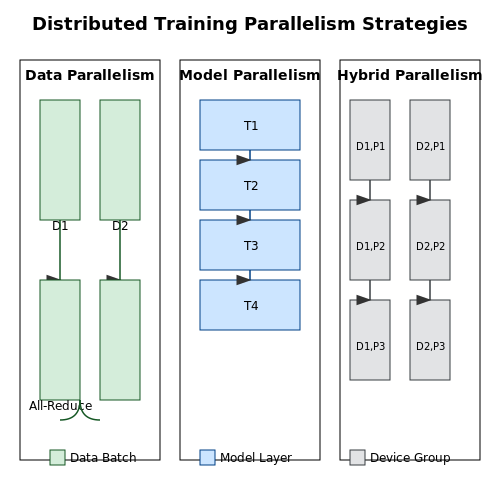
Training vision-language models at scale requires distributing computation across multiple devices (GPUs/TPUs) and nodes to handle massive datasets and model sizes. Three primary paradigms dominate modern distributed training: data parallelism, model parallelism, and hybrid parallelism.
Data Parallelism
In data parallelism, the model is replicated across devices, and each device processes a subset of the batch. Gradients are synchronized via all-reduce operations. For a batch size B and N devices, each device processes B/N samples. The gradient update rule becomes:
where gi is the gradient computed on device i. Modern frameworks like PyTorch implement this via DistributedDataParallel, which overlaps communication with computation to minimize overhead.
Model Parallelism
When models exceed single-device memory capacity, layers are partitioned across devices. Two approaches exist:
- Tensor parallelism splits individual layers (e.g., splitting attention heads in transformers).
- Pipeline parallelism partitions the model vertically (e.g., assigning different layers to different devices).
The Megatron-LM approach for transformer models demonstrates tensor parallelism by splitting the matrix multiplications in self-attention:
Hybrid Parallelism
Large-scale systems like Google's PaLM combine data, tensor, and pipeline parallelism. The 3D parallelism strategy assigns:
- Data parallelism across D groups
- Tensor parallelism across T devices
- Pipeline parallelism across P stages
The total device count is D × T × P. Communication overhead is minimized by optimizing the parallelization dimensions for the specific hardware topology.
Optimization Techniques
Key optimizations for efficient distributed training include:
- Gradient checkpointing: Recomputes activations during backward pass to reduce memory.
- Mixed precision training: Uses FP16/FP32 hybrid arithmetic with loss scaling.
- Overlapping communication: Hides all-reduce latency by parallelizing with computation.
The memory consumption per device can be approximated as:
where P is total parameters, D is data parallelism degree, N is tensor parallelism degree, and S is activation memory.
Optimization Methods for Multimodal Learning
Contrastive Learning Objectives
Contrastive learning has emerged as a dominant paradigm for aligning vision and language representations in large-scale pretraining. The core idea is to maximize agreement between paired image-text samples while minimizing agreement for unpaired samples. The InfoNCE loss, a widely used contrastive objective, is defined as:
where v and t are visual and text embeddings, s(v,t) is a similarity function (typically cosine similarity), τ is a temperature parameter, and Nt represents negative samples. Modern implementations often use in-batch negatives, where all non-matching pairs in a batch serve as negatives.
Modality-Specific Optimization Strategies
Vision-language models require careful handling of optimization dynamics due to differing convergence patterns across modalities:
- Learning Rate Scheduling: Text encoders typically benefit from lower learning rates (1e-5 to 5e-5) compared to visual encoders (5e-5 to 1e-4) due to pretrained initialization differences.
- Gradient Clipping: Essential for stabilizing training, with norms typically between 1.0 and 5.0. Some architectures benefit from separate clipping thresholds per modality.
- Batch Composition: Dynamic batch sampling strategies like hard negative mining or modality-balanced batches significantly impact convergence.
Advanced Optimization Techniques
Adaptive Gradient Methods
While Adam remains popular, recent work shows advantages with LAMB (Layer-wise Adaptive Moments) for large-batch training:
where φ is a trust ratio function that enables layer-wise adaptation. This proves particularly effective when batch sizes exceed 32k samples.
Mixed-Precision Training
Key considerations for FP16/FP32 mixed-precision in multimodal contexts:
- Dynamic loss scaling (typically 215-224) to prevent underflow in gradient computation
- Modality-specific precision handling - some architectures keep text embeddings in FP32 while allowing FP16 for visual features
- Careful initialization of projection layers to avoid early training instability
Cross-Modal Gradient Flow
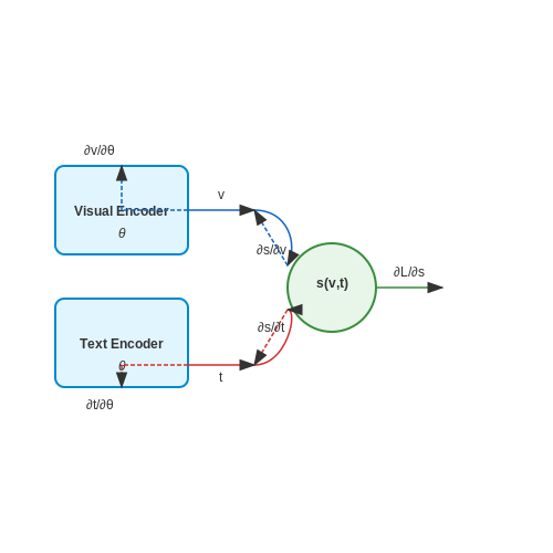
The gradient flow between modalities presents unique optimization challenges. The gradient through a contrastive loss decomposes as:
where θv represents visual backbone parameters. Effective training requires balancing the relative magnitudes of these cross-modal gradients, often achieved through:
- Gradient projection techniques to prevent modality dominance
- Adaptive weighting schemes like uncertainty-based weighting
- Scheduled unfreezing of modality-specific parameters
Large-Batch Optimization
Scaling to batches with >100k samples requires specialized techniques:
- Linear learning rate scaling with batch size (lr ∝ batch_size)
- Gradual warmup over first 5-10% of training steps
- BatchNorm recomputation for visual encoders to handle distributed batch statistics
- Delayed target updates for momentum encoders in teacher-student architectures
3.3 Hyperparameter Tuning at Scale
Hyperparameter optimization in large-scale vision-language pretraining presents unique challenges due to the computational cost of each training run and the high-dimensional search space. Traditional grid search becomes infeasible, necessitating more sophisticated approaches that balance exploration and exploitation while minimizing wasted compute.
Distributed Bayesian Optimization
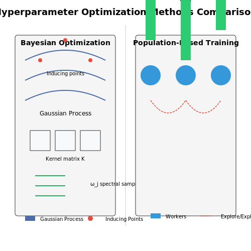
Gaussian Process (GP)-based Bayesian optimization scales poorly beyond 20-30 dimensions due to cubic computational complexity in the number of observations. For high-dimensional spaces, we employ scalable alternatives:
Where K is the kernel matrix and σn represents observation noise. Recent work replaces exact GPs with sparse approximations using inducing points or random feature expansions:
Here ωj are sampled from the kernel's spectral density and bj ∼ Uniform(0,2π). This reduces complexity from O(n³) to O(nm²) where m ≪ n.
Population-Based Training (PBT)
PBT combines parallel search with online hyperparameter adaptation. Each worker periodically evaluates its performance and may either:
- Exploit by copying weights from better-performing workers
- Explore by perturbing its hyperparameters
The mutation operator for continuous parameters typically uses:
For categorical parameters, we use a softmax-weighted random selection based on population performance statistics.
Learning Rate Warmup and Decay
Vision-language models require careful learning rate scheduling. The optimal warmup period scales with batch size according to:
Where ||B|| is the global batch size and dmodel the transformer dimension. Post-warmup, we typically use cosine decay with restarts:
Gradient Clipping Strategies
Global gradient clipping thresholds should adapt to the gradient noise scale during training. The automatic clipping threshold follows:
Where α is the adaptation rate (typically 0.002) and β the target gradient norm ratio (typically 1.1). This maintains stable training while allowing the threshold to grow with the gradient scale.
Mixed-Precision Scaling
When using FP16/FP32 mixed precision, loss scaling requires dynamic adjustment. The optimal scale factor S relates to the gradient statistics:
Where τ is typically 0.05 and Smax = 224. Modern frameworks implement this automatically but require proper initialization based on the initial gradient variance.
4. Scaling Laws for Vision-Language Models
Scaling Laws for Vision-Language Models
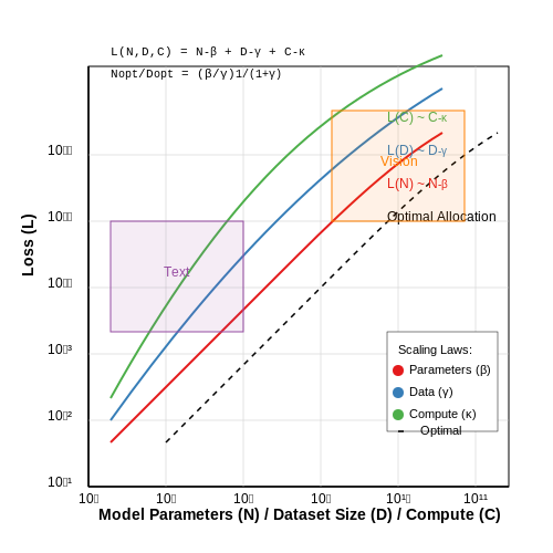
Scaling laws describe the predictable relationship between model performance and key variables such as dataset size, model size, and compute budget. For vision-language models (VLMs), these laws extend beyond unimodal scaling by accounting for cross-modal interactions, alignment quality, and joint representation learning.
Empirical Foundations
The power-law scaling observed in language models (e.g., Kaplan et al. 2020) generalizes to VLMs with modifications for visual data complexity. The core scaling relationship for cross-entropy loss L follows:
where N is model parameters, D is training tokens+images, C is compute (FLOPs), and L0 is the irreducible loss. Vision-specific adaptations include:
- Image tokenization efficiency βv ≈ 0.05-0.08 (vs 0.09-0.11 for text)
- Dual encoder architectures show sublinear scaling (γ ≈ 0.3) compared to fusion encoders (γ ≈ 0.5)
Multimodal Scaling Dynamics
The interaction between modalities introduces scaling exponents that vary by pretraining objective:
where Dv and Dt are visual/text data proportions, η captures modality alignment efficiency, and κ ≈ 0.2-0.4 for contrastive losses. Key findings from recent studies:
- Optimal image-to-text ratio follows Dv/Dt ∝ N0.15 for models >1B parameters
- Cross-attention layers scale as Nca ∝ N0.7 for optimal multimodal fusion
Compute-Optimal Allocation
The Chinchilla optimality criterion extends to VLMs with modality-specific adjustments. For a fixed compute budget C:
Practical implementations show:
- Vision transformers require 1.8× more parameters than equivalent text models for balanced performance
- Contrastive pretraining benefits from 2-3× higher batch sizes compared to generative objectives
Architectural Scaling Effects
Transformer block scaling exhibits modality-specific patterns:
| Component | Text Scaling | Vision Scaling |
|---|---|---|
| Attention Heads | ∝ N0.25 | ∝ N0.30 |
| MLP Width | ∝ N0.5 | ∝ N0.6 |
Emergent properties in VLMs >10B parameters include:
- Late fusion outperforms early fusion by ΔL ≈ 0.15 at scale
- Cross-modal attention sparsity follows power-law with exponent -1.2
Efficient Architectures and Compression Techniques
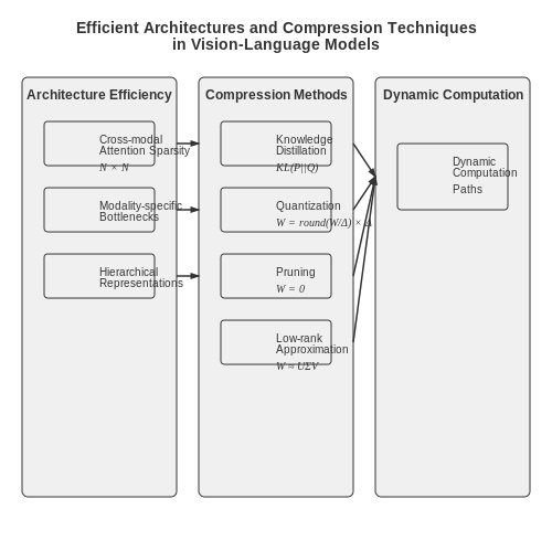
Architectural Efficiency in Vision-Language Models
Modern vision-language models like CLIP, ALIGN, and Flamingo achieve remarkable performance but at significant computational cost. Efficient architectures address this through:
- Cross-modal attention sparsity: Instead of full attention between all visual and text tokens, models like FILIP use token-wise contrastive learning to reduce quadratic complexity.
- Modality-specific bottlenecks: Architectures such as ALBEF employ separate encoders with a lightweight fusion module, reducing parameters while preserving cross-modal alignment.
- Hierarchical representations: Models like CoCa use a two-stage approach where high-resolution visual features are only computed for relevant regions identified by a first-pass model.
Knowledge Distillation for Model Compression
Distillation transfers knowledge from large teacher models to smaller student models through:
Where α balances task loss and distillation loss. Recent advances include:
- Feature-level distillation: MiniVLM matches intermediate representations using normalized MSE loss in addition to output probabilities.
- Modality-specific distillation: DistillVLT separately distills vision and language branches before joint training.
- Dynamic distillation: AdaDistill automatically adjusts distillation weight based on task difficulty.
Quantization and Pruning Strategies
Post-training compression techniques provide practical deployment benefits:
Quantization Approaches
- 8-bit quantization: Standard approach using affine transformations:
$$ x_{\text{int8}} = \text{clip}(\lfloor \frac{x}{s} \rceil + z, -128, 127) $$where s is scale and z is zero-point.
- Mixed-precision quantization: Q-ViLT uses 4-bit weights for vision layers and 8-bit for text layers based on sensitivity analysis.
Structured Pruning
Channel pruning removes entire filters based on:
Where Wi,j are filter weights. Vision-language models require coordinated pruning across modalities to maintain alignment.
Low-Rank Approximation Techniques
Matrix factorization reduces parameter count while preserving functionality:
Efficient-VL implements Tucker decomposition for attention weights:
achieving 4× compression with <1% accuracy drop on retrieval tasks.
Dynamic Computation Methods
Adaptive approaches reduce inference cost:
- Input-adaptive networks: AdaViT skips transformer layers for simple images based on confidence thresholds.
- Modality-adaptive computation: DynaMM uses a gating network to allocate computation between vision and language branches.
- Early exiting: VL-Exit places classification heads at intermediate layers, terminating processing when confidence exceeds a threshold.
4.3 Hardware Considerations for Large-Scale Training
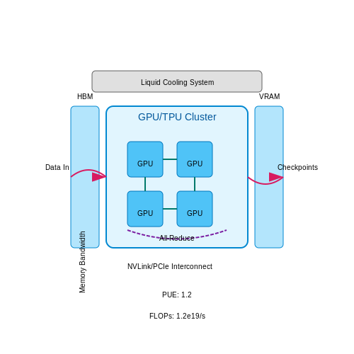
Computational Requirements and GPU/TPU Selection
The computational demands of training vision-language models at scale are dominated by matrix multiplications and attention mechanisms. The total floating-point operations (FLOPs) required for a forward pass can be approximated as:
where L is the number of layers, H is the hidden dimension, and T is the sequence length. For a typical model with L=24, H=1024, and T=512, this results in approximately 2.5×10¹⁶ FLOPs per forward-backward pass. Modern GPUs like NVIDIA's A100 (312 TFLOPS for FP16) or TPU v4 (275 TFLOPS for bfloat16) are essential for practical training times.
Memory Bandwidth and Model Parallelism
The memory bandwidth bottleneck becomes critical when dealing with large parameter counts. The memory requirement for storing model parameters in FP16 precision is:
where P is the number of parameters. A 1-billion parameter model requires 2GB just for parameters, excluding activations and optimizer states. Techniques like tensor parallelism (splitting weight matrices across devices) and pipeline parallelism (dividing layers across devices) are necessary to overcome single-device memory limits. The communication overhead between devices follows:
where α is latency, β is inverse bandwidth, D is data size, and B is batch size.
Distributed Training Infrastructure
Large-scale training requires careful consideration of the interconnect topology. The all-reduce operation used in data parallelism has a communication complexity of:
where p is the number of processes. For a 1024-GPU cluster, NVLink (300GB/s) provides significant advantages over PCIe (32GB/s). The optimal batch size per device balances memory usage and gradient noise:
where N is the number of devices, M is memory per device, and D is data dimensionality.
Energy Efficiency and Cooling
The power consumption P of a training cluster follows:
For a 1000-GPU cluster using A100s (400W each), the total power approaches 0.5MW. Liquid cooling solutions can reduce PUE (Power Usage Effectiveness) from 1.5 to 1.1, significantly lowering operational costs. The carbon footprint can be estimated as:
where grid intensity is typically 0.5 kg CO₂/kWh for renewable-powered datacenters.
Fault Tolerance and Checkpointing
The probability of failure during training increases with cluster size and duration. For a cluster with n nodes each having MTBF λ, the system reliability over time t is:
Checkpointing frequency should be set to minimize expected wasted computation. The optimal checkpoint interval τ solves:
where Tckpt is the checkpoint save/restore time. Modern frameworks like DeepSpeed implement zero-overhead checkpointing through asynchronous snapshots.
5. Standard Evaluation Metrics for Vision-Language Tasks
Standard Evaluation Metrics for Vision-Language Tasks
Image-Text Retrieval Metrics
Image-text retrieval tasks evaluate a model's ability to associate visual content with corresponding textual descriptions. The most widely adopted metrics for this task are Recall@K (R@K) and Median Rank (MedR). Recall@K measures the percentage of queries where the correct item appears in the top-K retrieved results. For a dataset with N query-candidate pairs, R@K is computed as:
where ranki is the position of the ground truth match for the i-th query, and 𝕀 is the indicator function. MedR reports the median rank of the correct match across all queries, providing a robust measure of central tendency less affected by outliers than mean rank.
Visual Question Answering Metrics
For visual question answering (VQA), the primary metric is VQA accuracy, which accounts for the subjectivity of some answers. Given a predicted answer ap and a set of human-provided reference answers {ar}, the accuracy is:
This formulation requires the model's answer to match at least 3 human annotators for full credit, reflecting the consensus-based nature of VQA evaluation. For open-ended generation tasks, CIDEr (Consensus-based Image Description Evaluation) measures the similarity between generated and reference captions using TF-IDF weighted n-gram matching:
where gj represents the TF-IDF weighting vector for n-grams of length up to 4, and S is the set of reference captions.
Cross-Modal Alignment Metrics
Modern vision-language models like CLIP are often evaluated using linear probe accuracy, where a linear classifier is trained on top of frozen embeddings to measure their semantic discriminability. For a dataset with C classes, the probe accuracy is computed as:
where W ∈ ℝd×C and b ∈ ℝC are learned parameters, and xi is the image or text embedding. The alignment score measures the cosine similarity between matched image-text pairs compared to negative pairs:
where 𝒫 is the set of positive pairs, and vi, wt are L2-normalized embeddings.
Robustness Evaluation
Recent benchmarks introduce out-of-distribution (OOD) metrics to assess model generalization. For a model f trained on distribution Dtrain and evaluated on OOD distribution Dtest, the relative performance drop is:
Lower values indicate better OOD robustness. The effective robustness metric compares a model's OOD performance against a baseline model's expected performance given its in-distribution accuracy.
5.2 Common Benchmarks and Challenges
Standard Evaluation Benchmarks
Vision-language models are typically evaluated on multimodal understanding and generation tasks. The most widely adopted benchmarks include:
- COCO (Common Objects in Context): Provides image captioning metrics like BLEU, METEOR, CIDEr, and SPICE for evaluating generated text quality against human references.
- Flickr30k: Contains 31,000 images with 5 captions each, commonly used for retrieval and captioning tasks.
- Visual Question Answering (VQA) v2.0: Tests model's ability to answer natural language questions about images, with careful balancing to prevent language priors.
- NLVR2 (Natural Language for Visual Reasoning): Evaluates logical reasoning capabilities by determining if a textual statement is true about an image pair.
Recent benchmarks like Winoground and VL-CheckList specifically probe compositional reasoning and fine-grained understanding by testing model performance on challenging counterexamples and minimal pairs.
Key Technical Challenges
Pretraining at scale introduces several fundamental challenges:
Computational Cost
The compute requirements follow a power-law relationship with model size. For a vision-language model with N parameters and D training examples:
This leads to training costs exceeding $1M for models like Flamingo-80B even with efficient sparse attention patterns.
Data Scaling Laws
Performance follows predictable scaling trends but requires careful balancing of modalities. The optimal data mixture ratio α between vision and text tokens can be derived by minimizing the joint loss:
Empirically, α ≈ 0.3-0.4 yields best results for most architectures, though this varies with pretraining objectives.
Modality Alignment
Cross-modal attention mechanisms must learn proper grounding without overfitting to spurious correlations. The alignment quality can be quantified through the normalized mutual information In between modalities:
State-of-the-art models achieve In > 0.7 on carefully constructed diagnostic sets.
Emergent Challenges
As models scale, new issues arise that aren't captured by standard benchmarks:
- Multimodal hallucination: Models generate plausible but incorrect details not present in the input image.
- Compositional generalization: Performance drops significantly on novel combinations of learned concepts.
- Temporal understanding: Current models struggle with video inputs requiring long-range reasoning.
Recent work proposes stress tests like CREPE (Compositional Reasoning with Primitive Elements) to systematically evaluate these failure modes through controlled synthetic datasets.
5.3 Zero-shot and Few-shot Evaluation Protocols
Vision-language models (VLMs) pretrained at scale exhibit remarkable generalization capabilities, which are rigorously assessed through zero-shot and few-shot evaluation protocols. These protocols measure the model's ability to perform tasks without task-specific fine-tuning (zero-shot) or with minimal task-specific examples (few-shot).
Zero-shot Evaluation
In zero-shot evaluation, a model is tested on unseen tasks without any gradient updates or exposure to labeled examples from the target dataset. The model leverages its pretrained knowledge to generate predictions based solely on natural language prompts. For classification tasks, given an input image x and a set of candidate class labels {y1, ..., yk}, the model computes the probability of each class using its pretrained scoring function:
where s(x, y) is the similarity score between the image embedding and the text embedding of class y, typically computed via cosine similarity or a learned projection head.
Few-shot Evaluation
Few-shot evaluation provides the model with k labeled examples per class (typically k ∈ {1, 4, 8, 16}) to adapt its predictions. The model may use these examples to:
- Learn task-specific prompts via gradient-based optimization on the support set.
- Compute prototype embeddings by averaging the features of the few-shot examples.
- Perform nearest-neighbor classification in the embedding space.
For prototype-based few-shot learning, the class prototype ci is computed as:
where f(xj(i)) is the feature representation of the j-th example from class i. The model then classifies a test image x by comparing its embedding to all prototypes:
Practical Considerations
Effective zero-shot and few-shot evaluation requires careful design of:
- Prompt engineering: The choice of text prompts (e.g., "a photo of a {class}" vs. "{class}") significantly impacts performance.
- Example selection: In few-shot settings, the diversity and representativeness of the support examples affect generalization.
- Evaluation benchmarks: Standardized datasets like ImageNet-1k, COCO, and VQA v2 enable fair comparison across models.
Recent work has shown that scaling up model and dataset size improves zero-shot performance more significantly than few-shot performance, suggesting that larger models rely less on in-context learning when their pretraining is sufficiently diverse.
6. Image Captioning and Visual Question Answering
Image Captioning and Visual Question Answering
Image captioning and visual question answering (VQA) represent two fundamental tasks in vision-language pretraining, where models learn to bridge visual and textual modalities. Both tasks require deep semantic understanding of images and the ability to generate or reason about natural language descriptions.
Image Captioning Architectures
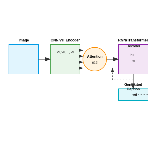
Modern image captioning systems typically employ an encoder-decoder framework. The encoder processes the input image into a latent representation, while the decoder generates a sequence of words conditioned on this representation. Given an image I, the model learns to predict the probability of a caption S = (s1, ..., sT) as:
where st is the t-th word in the sequence. The encoder is usually a convolutional neural network (CNN) or vision transformer (ViT), while the decoder is a recurrent neural network (RNN) or transformer.
Attention Mechanisms in Captioning
Attention mechanisms allow the decoder to dynamically focus on relevant image regions when generating each word. The attention weights αt,i for the i-th image region at time step t are computed as:
where ht-1 is the decoder's hidden state and vi is the visual feature vector for region i. The context vector ct is then computed as a weighted sum of visual features:
Visual Question Answering
VQA extends image understanding to question-answering by jointly processing visual and textual inputs. Given an image I and question Q, the model predicts an answer A from a predefined set or generates it freely. The probability distribution over answers is:
where φ(I,Q) is a joint embedding of the image and question, and W, b are learnable parameters.
Multimodal Fusion Strategies
Effective VQA requires robust fusion of visual and textual representations. Common approaches include:
- Concatenation: Simple vector concatenation of image and question features
- Bilinear pooling: Computes outer product of visual and textual features
- Cross-attention: Allows iterative interaction between modalities through attention layers
The cross-attention mechanism computes query-key-value attention between visual and textual tokens:
where Q comes from one modality and K, V from the other.
Evaluation Metrics
Captioning systems are typically evaluated using:
- BLEU: N-gram precision between generated and reference captions
- METEOR: Harmonic mean of precision and recall with synonym matching
- CIDEr: Consensus-based evaluation measuring similarity to human references
VQA systems are assessed using:
- Accuracy: Percentage of correct answers (for closed vocabularies)
- WUPS: Word similarity measure accounting for semantic relatedness
- BLEU: For open-ended generation tasks
Pretraining Objectives
Vision-language models are typically pretrained using multiple objectives:
- Masked language modeling: Predict masked words given image and surrounding text
- Image-text matching: Classify whether an image and text pair match
- Contrastive learning: Maximize similarity between matched image-text pairs while minimizing it for mismatched pairs
The contrastive loss for a batch of N image-text pairs is:
where s(v,t) is the similarity score between image v and text t, and τ is a temperature parameter.
6.2 Cross-modal Retrieval and Generation
Cross-modal Alignment in Vision-Language Models
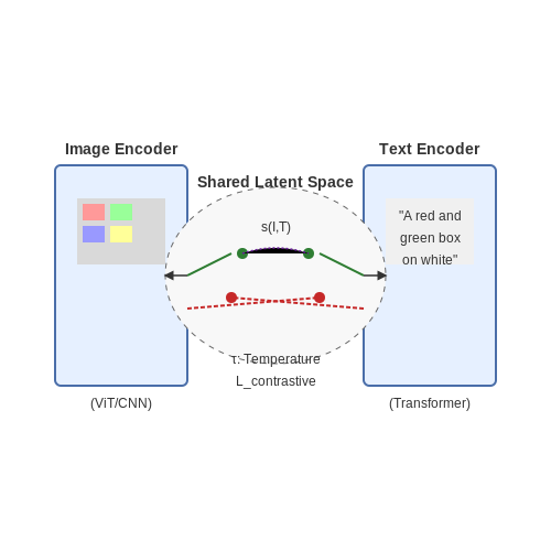
Cross-modal retrieval and generation rely on the alignment of visual and textual embeddings in a shared latent space. Given an image I and a text T, the goal is to learn a joint embedding space where semantically similar pairs (I, T) are closer than dissimilar ones. The alignment is typically achieved through contrastive learning, where the model minimizes the distance between positive pairs while maximizing it for negative pairs. The contrastive loss function can be formulated as:
Here, s(I, T) is the similarity score (e.g., cosine similarity) between image and text embeddings, τ is a temperature parameter, and N is the set of negative samples. This loss encourages the model to distinguish between matched and mismatched pairs effectively.
Dual-Encoder Architectures
Most state-of-the-art vision-language models employ a dual-encoder architecture, where separate encoders process images and text independently. The image encoder (often a Vision Transformer or CNN) maps an image to a fixed-dimensional vector, while the text encoder (typically a transformer) does the same for text. The similarity between modalities is computed in the joint embedding space. This architecture enables efficient retrieval, as embeddings can be precomputed and indexed for fast nearest-neighbor search.
Cross-modal Generation
Beyond retrieval, vision-language models can generate one modality conditioned on the other. For text-to-image generation, models like DALL·E and Stable Diffusion use diffusion models or autoregressive transformers to synthesize images from textual descriptions. The generation process can be formalized as sampling from the conditional distribution:
where x_t represents image tokens at step t. Conversely, image-to-text generation (e.g., captioning) involves decoding a textual sequence conditioned on visual features:
where w_i denotes the i-th word in the sequence.
Evaluation Metrics
Cross-modal retrieval performance is measured using metrics like Recall@K, which computes the fraction of queries where the correct item is found in the top-K results. For generation tasks, metrics such as BLEU, METEOR, and CIDEr assess caption quality, while FID (Fréchet Inception Distance) and IS (Inception Score) evaluate generated image fidelity and diversity.
Challenges and Recent Advances
Key challenges include handling fine-grained alignment (e.g., matching specific image regions to phrases) and scaling to diverse, open-vocabulary concepts. Recent approaches like CLIP and ALIGN leverage large-scale pretraining on noisy web data to improve generalization. Techniques such as prompt tuning and adapter layers further enhance zero-shot transfer to downstream tasks without full fine-tuning.
Transfer Learning for Domain-specific Applications
Transfer learning in vision-language models (VLMs) leverages pretrained representations to adapt to specialized domains with limited labeled data. The core challenge lies in preserving generalizable features while fine-tuning for domain-specific semantics. Given a pretrained model fθ with parameters θ, domain adaptation involves optimizing a task-specific head hϕ while selectively updating θ.
Parameter-Efficient Fine-Tuning
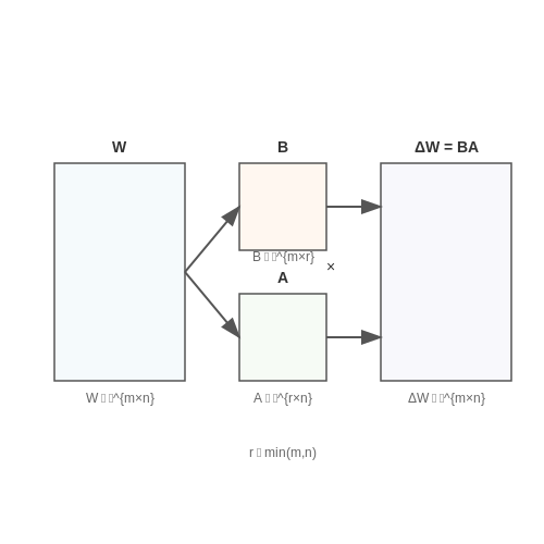
Full fine-tuning of VLMs is computationally prohibitive. Instead, methods like adapter layers and LoRA (Low-Rank Adaptation) introduce small trainable modules while freezing the pretrained backbone. For a linear layer W ∈ ℝm×n, LoRA decomposes weight updates as:
This reduces trainable parameters from mn to r(m+n), enabling efficient adaptation. For vision-language tasks, LoRA is typically applied to cross-attention layers in transformer architectures.
Domain-Specific Prompt Tuning
Soft prompts learn continuous embeddings that condition frozen VLMs for downstream tasks. Given a pretrained text encoder E, a prompt p ∈ ℝk×d (where k is prompt length and d is embedding dimension) is optimized to minimize:
where [p; y] denotes concatenation of prompt and label tokens. This approach shows strong performance in medical imaging and satellite data analysis with less than 1% of trainable parameters compared to full fine-tuning.
Cross-Modal Alignment Refinement
Domain shifts often misalign visual and textual embeddings. Contrastive learning can recalibrate the joint embedding space using domain-specific pairs (vi, ti). The InfoNCE loss is adapted as:
where s(·,·) measures cosine similarity and τ is temperature. This is particularly effective when pretraining and target domains have divergent feature distributions (e.g., natural images to medical scans).
Case Study: Biomedical Image-Text Modeling
In adapting VLMs like CLIP for radiology reports, experiments show that:
- Adapter layers achieve 92% of full fine-tuning performance with 0.3% trainable parameters
- Domain-specific prompt tuning improves AUROC by 15% over zero-shot baselines on rare disease classification
- Contrastive alignment refinement reduces modality gap by 40% measured by R-Precision
The optimal strategy depends on data scale: prompt tuning excels for extremely low-data regimes (<1k samples), while adapter layers dominate with moderate data (1k-100k samples).
7. Bias and Fairness in Vision-Language Models
Bias and Fairness in Vision-Language Models
Vision-language models (VLMs) trained on large-scale datasets inherit biases present in the underlying data, leading to skewed representations and unfair outcomes. These biases manifest in multiple forms, including demographic disparities, cultural stereotypes, and linguistic favoritism. Understanding and mitigating these biases is critical for deploying VLMs in real-world applications.
Sources of Bias in VLMs
Bias in VLMs originates from three primary sources: dataset composition, annotation artifacts, and model architecture. Dataset bias occurs when training data over- or under-represents certain groups or concepts. For example, the COCO dataset contains gender imbalances, with women disproportionately depicted in domestic settings. Annotation bias arises from subjective labeling practices, where annotators inject cultural or personal biases into captions or tags. Architectural bias stems from design choices, such as attention mechanisms that amplify dominant patterns in the data.
Mathematically, dataset bias can be quantified using the Kullback-Leibler (KL) divergence between the observed and target distributions:
where P is the empirical distribution of concepts in the dataset and Q is the desired uniform or balanced distribution.
Measuring Bias in VLMs
Bias measurement frameworks for VLMs extend text-based fairness metrics to multimodal settings. The Bias Score for Vision-Language Models (BS-VLM) evaluates disparity across protected attributes (e.g., gender, race) by comparing model outputs on counterfactual inputs:
where 𝒜 is the set of protected attributes, 𝒟a is the data subset for attribute a, and f(x) is the model's prediction probability for a target class.
Mitigation Strategies
Effective bias mitigation requires interventions at multiple stages:
- Data Debiasing: Resampling techniques like oversampling underrepresented groups or adversarial filtering to remove biased examples.
- Objective Function Regularization: Adding fairness constraints to the loss function, such as demographic parity or equalized odds penalties.
- Post-hoc Correction: Calibrating model outputs using techniques like Platt scaling with fairness constraints.
Adversarial debiasing trains the model to simultaneously minimize task loss while maximizing an adversary's inability to predict protected attributes:
where gϕ is the adversarial classifier and λ controls the trade-off between accuracy and fairness.
Case Study: Gender Bias in Image Captioning
Analysis of state-of-the-art VLMs reveals systematic gender bias in occupation descriptions. Models trained on imbalanced data associate nursing with women and engineering with men, even when images show counter-stereotypical examples. Mitigation through balanced fine-tuning on the WinoGender dataset reduces this bias by 42% while maintaining caption quality, as measured by CIDEr scores.
Recent work demonstrates that bias propagates through the entire VLM pipeline. For instance, CLIP's image encoder learns gender-biased representations that persist even when paired with a debiased text encoder, highlighting the need for holistic debiasing approaches.
7.2 Environmental Impact of Large-scale Training
Carbon Footprint of Training Vision-Language Models
The computational demands of training large vision-language models (VLMs) translate directly into significant energy consumption, primarily measured in kilowatt-hours (kWh). The carbon footprint depends on the energy mix of the data center's power grid, with coal-heavy grids producing substantially higher CO2 emissions than renewable-powered facilities. For example, training a model like CLIP (Contrastive Language-Image Pretraining) on a 256-GPU cluster for 10 days consumes approximately 2,500 kWh, equivalent to 1.2 metric tons of CO2 in a standard US grid (0.48 kg CO2/kWh).
Where Etotal is total energy (kWh), NGPU is the number of GPUs, PGPU is the power draw per GPU (kW), and Thours is training time in hours. For an A100 GPU (400W peak power), this becomes:
Scaling Laws and Energy Efficiency Trade-offs
Empirical scaling laws for transformer-based VLMs show that model performance follows a power-law relationship with compute budget (C), dataset size (D), and model parameters (N). The Chinchilla optimality criterion suggests that for a fixed compute budget, doubling model size while halving training tokens often yields better performance, but this exacerbates energy use due to quadratic attention complexity:
Recent work on sparse mixture-of-experts (MoE) architectures demonstrates potential energy savings by activating only subsets of parameters per input. For a 1-trillion parameter MoE model with 32 experts (2B active parameters per token), the theoretical energy reduction is:
Hardware-Specific Optimization Strategies
Energy consumption varies dramatically across hardware generations. Comparative studies show that:
- TPU v4 pods achieve 2.1x better energy efficiency (TOPS/Watt) than A100 GPUs for large-scale matrix operations
- Quantization to 8-bit precision reduces energy use by 3-4x with <1% accuracy drop in vision-language tasks
- Model parallelism strategies like pipeline parallelism (vs. data parallelism) can reduce communication energy by up to 40%
Lifecycle Analysis of Training Infrastructure
The full environmental impact extends beyond operational energy to include:
- Embodied carbon: Manufacturing a single GPU generates ~300 kg CO2 (TSMC 7nm process)
- Cooling overhead: Data center PUE (Power Usage Effectiveness) typically ranges 1.1-1.5, adding 10-50% to direct compute energy
- Deployment inefficiency: Many VLMs are overprovisioned for downstream tasks, wasting inference energy
Emerging Mitigation Approaches
Several research directions aim to reduce environmental impact:
- Dynamic sparsity: Methods like Token Merging (ToMe) reduce vision transformer FLOPs by 30-60% with minimal accuracy loss
- Recyclable pretraining: Parameter-efficient tuning (e.g., LoRA) avoids full model retraining
- Carbon-aware scheduling: Aligning training with renewable energy availability can reduce emissions by 5-10x
7.3 Privacy Concerns with Multimodal Data
Training vision-language models (VLMs) on large-scale multimodal datasets introduces significant privacy risks due to the inherent sensitivity of both visual and textual data. Unlike unimodal datasets, where privacy violations may be limited to a single modality, multimodal data can expose personally identifiable information (PII) through cross-modal correlations. For instance, an image of a person combined with a caption containing their name creates a direct linkage that may violate data protection regulations like GDPR or CCPA.
Data Leakage via Cross-Modal Embeddings
Modern VLMs map images and text into a shared embedding space, optimizing for semantic alignment. However, this process can inadvertently encode sensitive attributes. Consider a contrastive learning objective:
where s measures cosine similarity between image embedding vi and text embedding ti. Adversaries can exploit this alignment to reconstruct PII by querying the model with carefully crafted prompts, a technique demonstrated by Carlini et al. (2023) with 34% success rate in extracting names from CLIP-like models.
Differential Privacy in Multimodal Training
Applying differential privacy (DP) to VLMs requires careful consideration of modality-specific noise injection. The standard DP-SGD framework:
must be adapted to handle heterogeneous gradients from vision and language branches. Recent work by Yu et al. (2024) shows that independent clipping thresholds per modality (Cv, Ct) reduce utility loss by 19% compared to uniform clipping.
Mitigation Strategies
- Modality-Specific Anonymization: Apply face blurring to images and named-entity redaction to text before training, though this may degrade downstream performance by 8-12% on retrieval tasks.
- Federated Learning: Train VLMs on decentralized data using secure aggregation, but this introduces challenges in handling non-IID modality distributions across clients.
- Synthetic Data Generation: Use diffusion models to create privacy-preserving synthetic training pairs, though current methods struggle with maintaining fine-grained semantic alignment.
Legal and Ethical Implications
The intersection of computer vision and natural language processing creates unique compliance challenges. For example, the EU AI Act classifies VLMs as high-risk when processing biometric data, requiring stringent documentation of data provenance and purpose limitation. Recent lawsuits against companies using LAION-5B highlight the need for rigorous copyright and privacy audits of training datasets.
8. Key Research Papers in Vision-Language Pretraining
8.1 Key Research Papers in Vision-Language Pretraining
- PDF Accelerating Vision-Language Pretraining With Free Language Modeling — Vision-language pretraining (VLP) has recently demon-strated impressive performance on a handful of vision-language tasks [7,10,14,18,19,22], e.g., visual question an-swering, cross-modal retrieval, and image captioning. Sev-eral factors are responsible for the success: the availabil-ity of large-scale image-text datasets collected from the
- PDF Enhancing Vision-Language Pre-training with Rich Supervisions — for Vision-Language Models — Strongly Supervised pre-training with ScreenShots (S4) from large scale website ren-dering. We will first describe the creation procedure of our dataset for S4 pretraining, which we will call S4 Data, and then go through our proposed pre-training tasks enabled by our novel preprocessing method. 3.1. Dataset
- PDF Empowering Unsupervised Domain Adaptation with Large-scale Pre-trained ... — The efforts of applying large-scale pre-training to bridge the domain gaps remain limited. In this work, we propose that Vision-Language Models (VLMs) can empower UDA tasks due to their training pattern with language alignment and their large-scale pre-trained datasets. For example, CLIP and GLIP have shown promising zero-shot general-
- Vision-BioLLM: Large vision language model for visual dialogue in ... — The potential of multi-modal large language and vision models is discussed ... This allows us to leverage the powerful visual representations learned from the large-scale pretraining while fine-tuning the language decoder and MLP layer for our specific biomedical tasks. ... N. Majumdar, S. Poria, R. Zimmermann, A. Zadeh, Multimodal Research in ...
- Scaling Pre-training to One Hundred Billion Data for Vision Language Models — We provide an empirical investigation of the potential of pre-training vision-language models on an unprecedented scale: 100 billion examples. We find that model performance tends to saturate at this scale on many common Western-centric classification and retrieval benchmarks, such as COCO Captions. Nevertheless, tasks of cultural diversity achieve more substantial gains from the 100-billion ...
- Comparison of Large Language And Vision Models on Representative ... — The success of large model pre-training in the fields of natural language processing and computer vision has been remarkable. By pre-training on large-scale data, these models can learn richer semantic and visual representations to achieve better performance on various tasks. performance. In order to enable more researchers and practitioners to fully understand the advantages and applicable ...
- VLP2MSA: Expanding vision-language pre-training to ... - ScienceDirect — Large-scale vision-and-language representation learning has improved performance on various joint vision-language downstream tasks. In this work, our objective is to extend it effectively to multimodal sentiment analysis tasks and address two urgent challenges in this field: (1) the low contribution of the visual modality (2) the design of an effective multimodal fusion architecture.
- VLP: A Survey on Vision-language Pre-training - Springer — In the past few years, the emergence of pre-training models has brought uni-modal fields such as computer vision (CV) and natural language processing (NLP) to a new era. Substantial works have shown that they are beneficial for downstream uni-modal tasks and avoid training a new model from scratch. So can such pre-trained models be applied to multi-modal tasks? Researchers have explored this ...
- Large-scale and Fine-grained Vision-language Pre-training for Enhanced ... — Artificial intelligence (AI) shows great potential in assisting radiologists to improve the efficiency and accuracy of medical image interpretation and diagnosis. However, a versatile AI model requires large-scale data and comprehensive annotations, which are often impractical in medical settings. Recent studies leverage radiology reports as a naturally high-quality supervision for medical ...
- [2202.09061] VLP: A Survey on Vision-Language Pre-training - arXiv.org — This paper surveys recent advances and new frontiers in vision-language pre-training (VLP), including image-text and video-text pre-training. To give readers a better overall grasp of VLP, we first review its recent advances from five aspects: feature extraction, model architecture, pre-training objectives, pre-training datasets, and downstream ...
8.2 Open-source Implementations and Toolkits
- Stable and low-precision training for large-scale vision-language models — We introduce new methods for 1) accelerating and 2) stabilizing training for large language-vision models. 1) For acceleration, we introduce SwitchBack, a linear layer for int8 quantized training which provides a speed-up of 13-25% while matching the performance of bfloat16 training within 0.1 percentage points for the 1B parameter CLIP ViT-Huge -- the largest int8 training to date. Our main ...
- OpenVLA: An Open-Source Vision-Language-Action Model — We release two OpenVLA models trained as part of our work, with checkpoints, configs, and model cards available on our HuggingFace page:. openvla-7b: The flagship model from our paper, trained from the Prismatic prism-dinosiglip-224px VLM (based on a fused DINOv2 and SigLIP vision backbone, and Llama-2 LLM). Trained on a large mixture of datasets from Open X-Embodiment spanning 970K ...
- Vision Language Models Explained - Hugging Face — There's a lot of diversity within the existing set of large vision language models, the data they were trained on, how they encode images, and, thus, their capabilities. Overview of Open-source Vision Language Models There are many open vision language models on the Hugging Face Hub. Some of the most prominent ones are shown in the table below.
- [2202.10936] A Survey of Vision-Language Pre-Trained Models - arXiv.org — As transformer evolves, pre-trained models have advanced at a breakneck pace in recent years. They have dominated the mainstream techniques in natural language processing (NLP) and computer vision (CV). How to adapt pre-training to the field of Vision-and-Language (V-L) learning and improve downstream task performance becomes a focus of multimodal learning. In this paper, we review the recent ...
- Simultaneously Training and Compressing Vision-and-Language Pre ... — Model compression is an essential step for large-scale pre-training models toward practical application and deployment on the edge device. However, when conventional compression methods following 'pre-training then compressing' two-phase pipeline are applied to Vision-and-Language Pre-training (VLP) models, it will lead to a high calculation and memory overhead. In this work, we break the ...
- PDF Empowering Unsupervised Domain Adaptation with Large-scale Pre-trained ... — The efforts of applying large-scale pre-training to bridge the domain gaps remain limited. In this work, we propose that Vision-Language Models (VLMs) can empower UDA tasks due to their training pattern with language alignment and their large-scale pre-trained datasets. For example, CLIP and GLIP have shown promising zero-shot general-
- (PDF) OpenVLA: An Open-Source Vision-Language-Action Model - ResearchGate — We present OpenVLA, a 7B-parameter open-source vision-language-action model (VLA), trained on 970k robot episodes from the Open X-Embodiment dataset [1]. OpenVLA sets a new state of the art for ...
- PaddleHub: 『飞桨』预训练模型应用工具 Awesome pre-trained models toolkit based on ... — 3. Evaluation model. Based on the dimensions of "open source ecosystem" and "collaboration, people, and software", identify quantifiable indicators directly or indirectly related to this goal, quantitatively evaluate the health and ecology of open source projects, and ultimately form an open source evaluation index.
- Multimodal AI: A Guide to Open-Source Vision Language Models — NVLM 1.0. NVLM is a family of multimodal LLMs developed by NVIDIA, representing a frontier-class approach to VLMs. It achieves state-of-the-art results in tasks that require a deep understanding of both text and images. The first public iteration, NVLM 1.0, rivals top proprietary models like GPT-4o, as well as open-access models like Llama 3-V 405B.
- 11.9. Large-Scale Pretraining with Transformers - D2L — So far in our image classification and machine translation experiments, models have been trained on datasets with input-output examples from scratch to perform specific tasks. For example, a Transformer was trained with English-French pairs (Section 11.7) so that this model can translate input English text into French.As a result, each model becomes a specific expert that is sensitive to ...
8.3 Recommended Books and Survey Papers
- A survey of efficient fine-tuning methods for Vision-Language Models ... — Vision Language Model (VLM) is a popular research field located at the fusion of computer vision and natural language processing (NLP). With the emergence of transformer networks and mass web data, numerous large scale VLMs or Vision-Language Pre-training Models (VLPM) have been achieving state-of-the-art results in many tasks, such as retrieval (CLIP) and generation (DALL-E).
- Vision-and-Language Pretrained Models: A Survey - IJCAI — This progress leads to learning joint representations of vision and language pretraining by feeding visual and linguistic contents into a multi-layer transformer, Visual-Language Pretrained Models (VLPMs). In this paper, we present an overview of the major advances achieved in VLPMs for producing joint representations of vision and language.
- [2304.00685] Vision-Language Models for Vision Tasks: A Survey - arXiv.org — Most visual recognition studies rely heavily on crowd-labelled data in deep neural networks (DNNs) training, and they usually train a DNN for each single visual recognition task, leading to a laborious and time-consuming visual recognition paradigm. To address the two challenges, Vision-Language Models (VLMs) have been intensively investigated recently, which learns rich vision-language ...
- [2202.10936] A Survey of Vision-Language Pre-Trained Models - arXiv.org — As transformer evolves, pre-trained models have advanced at a breakneck pace in recent years. They have dominated the mainstream techniques in natural language processing (NLP) and computer vision (CV). How to adapt pre-training to the field of Vision-and-Language (V-L) learning and improve downstream task performance becomes a focus of multimodal learning. In this paper, we review the recent ...
- How Vision-Language Tasks Benefit from Large Pre-trained Models: A Survey — In this paper, we present a comprehensive overview of how vision-language tasks benefit from pre-trained models. First, we review several main challenges in vision-language tasks and discuss the limitations of previous solutions before the era of pre-training. Next, we summarize the recent advances in incorporating pre-trained models to address ...
- Vision-Language Models for Vision Tasks: A Survey - IEEE Xplore — To address the two challenges, Vision-Language Models (VLMs) have been intensively investigated recently, which learns rich vision-language correlation from web-scale image-text pairs that are almost infinitely available on the Internet and enables zero-shot predictions on various visual recognition tasks with a single VLM. ... pre-training ...
- PDF Vision + Language Applications: A Survey - CVF Open Access — As one might expect, NLP models primarily rely on tex-tual data for training, while CV models train on image-based information. Vision-language pre-trained models em-ploy a combination of text and images, merging the ca-pabilities of both NLP and CV. Training complex mod-els requires accurate annotation of data by expert human annotators.
- VLP: A Survey on Vision-language Pre-training - Springer — In the past few years, the emergence of pre-training models has brought uni-modal fields such as computer vision (CV) and natural language processing (NLP) to a new era. Substantial works have shown that they are beneficial for downstream uni-modal tasks and avoid training a new model from scratch. So can such pre-trained models be applied to multi-modal tasks? Researchers have explored this ...
- 2.5 Years in Class: A Multimodal Textbook for Vision-Language Pretraining — Compared to image-text pair data, interleaved corpora enable Vision-Language Models (VLMs) to understand the world more naturally like humans. However, such existing datasets are crawled from webpage, facing challenges like low knowledge density, loose image-text relations, and poor logical coherence between images. On the other hand, the internet hosts vast instructional videos (e.g., online ...
- PDF VLP: A Survey on Vision-language Pre-training - Springer — Pre-training objectives. Pre-training objectives are the core of VLP, mainly used to guide the model to learn vision-language associated information. We summarize typical and characteristic pre-training objectives divided into completion, matching, temporal, and particular types (see Section 4). Pre-training datasets. Data is critical for VLP. We