Multi-modal Retrieval Systems
1. Definition and Core Concepts
Definition and Core Concepts
Multi-modal retrieval systems are designed to search and retrieve information across multiple data modalities—such as text, images, audio, and video—by leveraging their inherent relationships. Unlike unimodal systems, which operate within a single data type, multi-modal retrieval requires joint embedding spaces where different modalities can be compared directly. The core challenge lies in aligning heterogeneous representations while preserving semantic consistency.
Modality Alignment
Effective multi-modal retrieval hinges on modality alignment, where embeddings from different data types are projected into a shared latent space. Given two modalities A and B, the objective is to minimize the distance between corresponding pairs (ai, bi) while maximizing separation for non-matching pairs. A common approach involves contrastive learning with triplet loss:
where d(·,·) is a distance metric (e.g., cosine similarity), f is the embedding function, and α is a margin hyperparameter. Advanced methods like cross-modal attention further refine alignment by dynamically weighting inter-modal features.
Joint Embedding Spaces
A joint embedding space enables direct comparison across modalities by mapping them to a unified representation. For instance, CLIP (Contrastive Language-Image Pretraining) aligns images and text using a dual-encoder architecture:
where EI and ET are trained to maximize the similarity between matched image-text pairs (vi, ti). The similarity score is computed as:
Cross-Modal Fusion
For tasks requiring combined modality inputs (e.g., video retrieval with audio-visual cues), cross-modal fusion integrates features before retrieval. Techniques include:
- Early Fusion: Concatenates raw features before embedding, e.g., f([ai; bi]).
- Late Fusion: Combines modality-specific embeddings post-hoc, often via weighted averaging or attention mechanisms.
Transformer-based architectures, such as ViLBERT, leverage co-attention layers to model interdependencies between modalities dynamically.
Evaluation Metrics
Performance is quantified using cross-modal retrieval metrics:
- Recall@K: Proportion of queries where the correct item is in the top-K results.
- Mean Reciprocal Rank (MRR): Average reciprocal rank of the first correct result across queries.
For datasets like MS-COCO or AudioSet, benchmarks often report R-Precision (precision at R, where R is the number of relevant items per query).
Key Components of Multi-modal Systems
Embedding Spaces and Alignment
Multi-modal retrieval systems rely on embedding spaces where different modalities (text, image, audio) are projected into a shared latent space. The core challenge is ensuring semantic alignment across modalities. Given two modalities A and B, the objective is to learn mappings fA and fB such that:
where a and b are samples from modalities A and B, respectively. Contrastive learning frameworks like CLIP employ triplet loss to minimize distances between positive pairs while maximizing separation for negative pairs:
Cross-Modal Attention Mechanisms
Transformer-based architectures enable dynamic interaction between modalities through cross-attention layers. For a query q from modality A and key-value pairs (k, v) from modality B, attention weights are computed as:
This allows the model to attend to relevant regions in B when processing A, crucial for tasks like visual question answering. The output is a weighted sum of values vj based on these attention scores.
Modality-Specific Encoders
Each modality requires specialized encoding architectures:
- Text: Pretrained language models (BERT, GPT) with token embeddings and positional encoding
- Images: CNN backbones (ResNet) or vision transformers (ViT) with patch embeddings
- Audio: Spectrogram processing via 1D convolutions or mel-frequency cepstral coefficients
These encoders must preserve intra-modal relationships while enabling cross-modal comparison. For instance, ViT divides images into 16x16 patches, linearly projected into tokens compatible with transformer architectures.
Fusion Strategies
Late fusion combines modality-specific features after independent processing, while early fusion processes raw inputs jointly. Hybrid approaches like cross-modal transformers implement intermediate fusion through attention layers. The choice depends on computational constraints and task requirements:
| Fusion Type | Advantages | Disadvantages |
|---|---|---|
| Early | Captures fine-grained interactions | High memory usage |
| Late | Modular and scalable | Loses low-level correlations |
Retrieval Indexing
Approximate nearest neighbor (ANN) search enables efficient retrieval in high-dimensional spaces. Hierarchical navigable small world (HNSW) graphs provide logarithmic-time lookup by constructing layered proximity graphs. For a dataset of size N, HNSW achieves O(log N) query time with recall rates exceeding 90% for top-100 retrieval.
where Truek are the ground truth nearest neighbors. Modern systems combine ANN with learned metrics to optimize for task-specific similarity.

1.3 Challenges in Multi-modal Retrieval
Heterogeneous Data Representation
Multi-modal retrieval systems must process data from diverse modalities—text, images, audio, video—each with distinct feature spaces and dimensionalities. For instance, text is typically represented in high-dimensional sparse vectors (e.g., TF-IDF or word embeddings), while images are encoded as dense tensors via CNNs. The fundamental challenge lies in projecting these heterogeneous representations into a unified embedding space where cross-modal similarity can be computed. Mathematically, given modalities A and B, the goal is to learn mappings fA and fB such that:
Optimizing these mappings requires solving non-convex objectives with constraints on geometric alignment, often leading to unstable training dynamics.
Semantic Gaps and Alignment
Modalities often capture complementary but non-overlapping semantic information. A photo of a "dog running" might lack the explicit temporal context present in a corresponding video clip. Bridging this gap demands joint embedding techniques that preserve both intra-modal and cross-modal relationships. Contrastive learning frameworks like CLIP have shown promise, but they struggle with fine-grained alignment—e.g., matching a textual description of "a red car turning left" to the exact frame in a video where this action occurs.
Scalability and Latency
Real-time retrieval across billions of multi-modal items introduces computational bottlenecks. Approximate nearest neighbor (ANN) search algorithms like HNSW or IVF must balance recall against query latency when handling high-dimensional embeddings. The computational complexity grows exponentially with embedding dimensionality d:
where N is the dataset size and k is the number of retrieved items. This becomes prohibitive when d exceeds 1024 dimensions—common in modern vision-language models.
Noise and Missing Modalities
Real-world datasets often contain corrupted or missing modalities (e.g., silent videos or images with occluded text). Robust retrieval requires either imputation strategies or architectures that dynamically reweight modalities based on availability. Recent work employs attention mechanisms to compute modality importance scores αi:
where hi are modality-specific features and w is a learnable weight vector.
Evaluation Metrics
Traditional single-modal metrics (e.g., precision@k) fail to capture cross-modal retrieval quality. Multi-modal extensions like:
- Cross-modal retrieval accuracy (CMRA): Ratio of queries where the true match ranks in the top-k results across modalities
- Mean reciprocal rank (MRR): Harmonic mean of reciprocal ranks of correct matches
- R-Precision: Precision at R, where R is the number of relevant items per query
require carefully constructed evaluation protocols to avoid dataset-specific biases.
Dynamic Modality Interaction
In interactive systems, user feedback (e.g., relevance judgments) should dynamically refine retrieval. This necessitates online learning of the joint embedding space, posing challenges in catastrophic forgetting—where updating the model for one modality degrades performance on others. Techniques like elastic weight consolidation (EWC) add regularization terms to preserve important parameters:
where Fi is the Fisher information matrix diagonal for parameter θi.

2. Feature Extraction for Different Modalities
Feature Extraction for Different Modalities
Text Modality: Embedding Techniques
Text feature extraction transforms unstructured language into dense vector representations. Transformer-based models like BERT and GPT employ self-attention mechanisms to capture contextual relationships. Given an input sequence X = [x1, ..., xn], the self-attention score between tokens xi and xj is computed as:
where Q, K, and V are learned query, key, and value matrices, and dk is the dimension of the key vectors. State-of-the-art models like Sentence-BERT fine-tune this mechanism for semantic similarity tasks by optimizing a triplet loss:
where fa, fp, and fn are embeddings for anchor, positive, and negative samples.
Image Modality: Convolutional and Vision Transformers
For images, convolutional neural networks (CNNs) extract hierarchical features through learned filters. A 2D convolution operation at layer l is defined as:
where Wl is the filter kernel of size (2k+1)×(2k+1). Vision Transformers (ViTs) partition images into patches pi ∈ ℝP×P×3, linearly project them, and process via multi-head attention:
where E is the patch embedding matrix and Epos encodes positional information.
Audio Modality: Spectrogram Representations
Audio signals are often transformed into time-frequency representations using Short-Time Fourier Transforms (STFT):
where w(n) is the window function and H is the hop size. Learned architectures like Wav2Vec 2.0 use convolutional feature encoders followed by transformer layers to model temporal dependencies:
Cross-Modal Alignment
Contrastive learning frameworks like CLIP align embeddings across modalities by maximizing mutual information. Given image-text pairs (I, T), the contrastive loss is:
where τ is a temperature parameter and sim(·) is cosine similarity. This enables zero-shot retrieval by projecting queries and candidates into a shared embedding space.
Feature Fusion Strategies
Late fusion combines unimodal features through concatenation or attention mechanisms. For modalities M1, M2, cross-modal attention computes:
where QM1, KM2, VM2 are derived from modality-specific projections.

2.2 Cross-modal Embedding Methods
Foundations of Cross-modal Alignment
Cross-modal embedding methods aim to project data from different modalities (e.g., text, images, audio) into a shared latent space where semantically similar items are close regardless of their original form. The core challenge lies in preserving both intra-modal relationships and inter-modal correspondences. Let X and Y represent feature spaces for two modalities, with paired samples (xi, yi). The objective is to learn mappings f: X → Z and g: Y → Z that minimize:
where dz is a distance metric in the shared space Z, and δij indicates whether (xi, yj) are paired. Advanced implementations often employ triplet loss or contrastive learning to handle unpaired data.
Canonical Correlation Analysis (CCA) Extensions
Traditional CCA finds linear projections that maximize correlation between modalities. For nonlinear relationships, kernel CKA (Centered Kernel Alignment) extends this via reproducing kernel Hilbert spaces:
where Kx and Ky are kernel matrices. DeepCCA further generalizes this using neural networks to learn nonlinear transformations, achieving state-of-the-art results on tasks like audiovisual speech recognition.
Neural Network Architectures
Modern approaches leverage dual-stream architectures with modality-specific encoders:
The training typically involves:
- Contrastive loss: Pulls positive pairs together while pushing negatives apart
- Cross-modal reconstruction: Auxiliary decoders enforce semantic consistency
- Adversarial alignment: Discriminators ensure indistinguishable distributions in Z
Attention Mechanisms in Cross-modal Retrieval
Transformer-based models like CLIP employ cross-attention to dynamically weight relevant features across modalities. For a query q and key-value pairs (K, V) from another modality:
This allows fine-grained alignment, such as associating image regions with specific words in captions. The ViLBERT model demonstrates this by achieving 12.7% improvement over non-attentive baselines on visual question answering.
Evaluation Metrics
Performance is quantified through:
- Recall@K: Probability of true matches appearing in top-K retrievals
- Mean Reciprocal Rank (MRR): Harmonic mean of reciprocal ranks of correct results
- Modality Blending Score: Measures how well the space preserves within-modality relationships while enabling cross-modal queries
State-of-the-art models on MS-COCO achieve R@1 of 58.4% for image-to-text and 43.9% for text-to-image retrieval using hybrid contrastive-probabilistic objectives.

Early, Late, and Hybrid Fusion Strategies
Early Fusion (Feature-Level Fusion)
Early fusion combines raw or low-level features from different modalities before feeding them into a retrieval model. Given two modalities A and B with feature vectors fA and fB, early fusion concatenates them into a single joint representation:
This approach is effective when modalities have strong inter-dependencies, as the model learns cross-modal correlations directly from raw features. However, early fusion suffers from the curse of dimensionality when dealing with high-dimensional features, and synchronization of heterogeneous data streams can be challenging.
Late Fusion (Score-Level Fusion)
Late fusion processes each modality independently and combines their outputs (e.g., similarity scores or decision probabilities) at the final stage. For retrieval tasks, given modality-specific similarity scores SA and SB, late fusion computes a weighted combination:
where α is a learnable or fixed weighting parameter. Late fusion is computationally efficient and robust to missing modalities, but it cannot capture fine-grained cross-modal interactions since modalities are processed in isolation.
Hybrid Fusion
Hybrid strategies combine the strengths of early and late fusion. A common approach is to:
- Perform early fusion on subsets of related modalities
- Process remaining modalities independently
- Fuse all intermediate representations at multiple levels
For example, in a vision-language retrieval system, visual and textual features might first be fused early via cross-attention, then combined with late-fused audio features through a gating mechanism:
where hvl is the vision-language joint representation, ha is the audio embedding, Wg is a learnable weight matrix, and σ is a sigmoid activation.
Practical Considerations
Choice of fusion strategy depends on:
- Modality relationships: Early fusion works best for tightly-coupled modalities (e.g., video+audio), while late fusion suits independent modalities
- Computational constraints: Early fusion requires more memory due to concatenated features
- Data availability: Late fusion handles missing modalities more gracefully
State-of-the-art systems like CLIP and Flamingo employ sophisticated hybrid approaches, using cross-modal transformers for early interaction while maintaining separate encoders for modality-specific processing.

3. Neural Network-based Approaches
3.1 Neural Network-based Approaches
Neural network-based approaches dominate modern multi-modal retrieval systems due to their ability to learn joint embeddings from heterogeneous data sources. These models typically employ deep architectures that project different modalities into a shared latent space where similarity can be computed directly. The key innovation lies in their capacity to capture non-linear relationships and high-level semantic correlations that traditional methods often miss.
Cross-Modal Embedding Architectures
The foundational architecture for neural multi-modal retrieval consists of twin neural networks—one per modality—trained to minimize a similarity-based loss function. Given two modalities A and B, the networks fA and fB produce embeddings where semantically similar pairs (ai, bi) are closer in the latent space than dissimilar pairs. The training objective can be formulated as:
where S is a similarity metric (typically cosine similarity) and α is a margin hyperparameter. This triplet loss formulation forces the network to separate positive pairs from negatives by at least margin α.
Attention Mechanisms in Multi-Modal Retrieval
Modern systems incorporate attention mechanisms to dynamically weight the importance of different regions or features within each modality. For image-text retrieval, this allows the model to focus on relevant image patches when processing a query caption. The attention weights αij between image region i and word j are computed as:
where vi represents visual features and wj textual features. This soft alignment enables more precise retrieval by modeling fine-grained inter-modal relationships.
Transformer-Based Approaches
Recent advances leverage transformer architectures to process multiple modalities simultaneously. Models like CLIP and ALIGN use a dual-encoder framework where:
- Image encoder: Typically a Vision Transformer (ViT) or ResNet backbone
- Text encoder: A transformer-based language model (e.g., BERT)
These models are pre-trained on massive datasets using contrastive learning objectives, achieving remarkable zero-shot retrieval capabilities. The training objective maximizes the similarity between correct image-text pairs while minimizing it for incorrect ones:
where τ is a temperature parameter controlling the sharpness of the distribution.
Practical Implementation Considerations
When implementing neural retrieval systems, several architectural choices significantly impact performance:
- Embedding dimensionality: Typically 512-1024 dimensions balances expressiveness and efficiency
- Normalization: L2-normalizing embeddings before similarity computation stabilizes training
- Negative mining: Hard negative mining strategies improve convergence by focusing on challenging examples
- Asymmetric architectures: Allowing different network depths per modality can better handle modality-specific complexities
Recent benchmarks on MS-COCO and Flickr30K datasets show neural approaches achieving recall@1 scores above 60% for image-to-text retrieval, significantly outperforming traditional methods. The field continues to advance with techniques like cross-modal distillation and modality-agnostic transformers pushing performance boundaries further.

3.2 Transformer Models in Multi-modal Retrieval
Transformer architectures have revolutionized multi-modal retrieval by enabling joint representation learning across heterogeneous data modalities. The self-attention mechanism allows the model to dynamically weigh the importance of different tokens or features within and across modalities, making it particularly effective for tasks like cross-modal search, image-text matching, and video-audio retrieval.
Architectural Adaptations for Multi-modality
Standard transformer models require modifications to handle multi-modal inputs effectively. The key adaptations include:
- Modality-specific encoders: Separate transformer branches process each input modality (text, image, audio) before fusion.
- Cross-modal attention layers: Special attention heads compute interactions between tokens from different modalities.
- Shared embedding spaces: Projections align representations from different modalities into a common vector space.
The cross-modal attention can be formalized as:
where Q, K, and V can come from different modalities. For example, in image-text retrieval, Q might represent image region features while K and V represent text tokens.
Training Objectives
Multi-modal transformers typically employ contrastive learning objectives to align representations across modalities:
where s(v,t) computes the similarity between visual and textual embeddings, and τ is a temperature hyperparameter. This objective pushes matching image-text pairs closer in the embedding space while separating non-matching pairs.
Efficient Retrieval with Transformers
For large-scale retrieval, transformer models face computational challenges due to their quadratic attention complexity. Several approaches address this:
- Token pruning: Removing less informative tokens early in the network.
- Cross-modal late interaction: Computing attention only between compressed representations.
- Approximate nearest neighbor search: Using techniques like HNSW over transformer embeddings.
The retrieval process typically involves two phases: an initial broad search using approximate methods followed by a re-ranking stage with full transformer inference on candidate pairs.
Case Study: CLIP for Multi-modal Retrieval
OpenAI's CLIP model demonstrates the effectiveness of transformer architectures for multi-modal retrieval. The model achieves zero-shot transfer to downstream retrieval tasks through:
- A dual-encoder architecture with separate image and text transformers
- Contrastive pre-training on 400 million image-text pairs
- Shared embedding space enabling direct comparison across modalities
CLIP's success highlights how large-scale transformer training can create highly generalizable multi-modal representations suitable for diverse retrieval applications.

Graph-based Retrieval Methods
Graph-based retrieval methods leverage structured representations of data as nodes and edges to capture complex relationships between multi-modal entities. Unlike vector-based approaches, which rely on dense embeddings, graph methods explicitly model semantic, spatial, or temporal dependencies, enabling more interpretable and flexible retrieval.
Graph Construction and Representation
Given a multi-modal dataset, entities (e.g., images, text snippets, or audio clips) are represented as nodes V in a graph G = (V, E), where edges E encode relationships. Edge weights can be derived from:
- Semantic similarity (e.g., cosine similarity between text embeddings)
- Co-occurrence statistics (e.g., images and captions appearing together)
- Domain-specific constraints (e.g., spatial proximity in video frames)
where sim(vi, vj) is a similarity function and 𝒩(i) denotes the neighborhood of node i.
Random Walk with Restarts (RWR)
RWR computes relevance scores by simulating a Markov process on the graph. The transition probability matrix P is defined as:
The steady-state distribution r, obtained via iterative updates, gives the relevance of nodes to a query q:
where α controls the restart probability. This method is particularly effective for cross-modal retrieval, where queries and targets reside in different modalities.
Graph Neural Networks (GNNs)
Modern approaches employ GNNs to learn node embeddings that encode both content and graph structure. A typical Graph Convolutional Network (GCN) layer updates node features as:
where  = A + I (adjacency matrix with self-loops), D̂ is the degree matrix, and W(l) are learnable weights. Multi-layer GNNs propagate information across k-hop neighborhoods, capturing higher-order relationships.
Applications and Case Studies
- Visual Question Answering: Scene graphs connect objects (nodes) with spatial/predicate relations (edges), improving answer retrieval.
- Recommendation Systems: User-item interaction graphs enable personalized retrieval via RWR or GNNs.
- Biomedical Knowledge Graphs: Drug-protein-disease networks support multi-modal evidence retrieval for clinical decision-making.
Hybrid methods combining graph-based and vector-based retrieval (e.g., Dense Retrieval with Graph Reranking) often achieve state-of-the-art performance by leveraging the strengths of both paradigms.

4. Standard Metrics for Retrieval Performance
4.1 Standard Metrics for Retrieval Performance
Precision and Recall
Precision and recall form the foundation of retrieval evaluation. Precision measures the fraction of retrieved items that are relevant, while recall quantifies the fraction of relevant items successfully retrieved from the entire corpus. For a given query q, these metrics are defined as:
In multi-modal systems, relevance judgments must account for cross-modal alignment, where an image and its corresponding text caption may be considered a relevant pair. Precision and recall are particularly sensitive to the ranking threshold, making them useful for binary retrieval tasks but less informative for ranked retrieval scenarios.
Average Precision (AP) and Mean Average Precision (MAP)
Average Precision extends precision by considering the order of retrieved items. For a single query, AP is computed as the average of precision values at each relevant item's rank position:
where rel(k) is 1 if the item at rank k is relevant, and 0 otherwise. MAP aggregates AP across multiple queries:
MAP is widely used in benchmarks like MS-COCO and Flickr30k, where it captures both the completeness and ranking quality of retrieval results.
Normalized Discounted Cumulative Gain (nDCG)
nDCG evaluates ranked lists by accounting for graded relevance (e.g., strongly relevant, somewhat relevant). The Discounted Cumulative Gain (DCG) at rank k is:
where reli is the relevance score of the item at position i. nDCG normalizes DCG by the ideal DCG (IDCG), which is the maximum possible DCG for a perfect ranking:
nDCG is particularly useful for multi-modal retrieval, where relevance may be continuous (e.g., similarity scores between embeddings).
Recall@K and Precision@K
These truncated metrics evaluate performance at a fixed cutoff K. Recall@K measures the fraction of relevant items found in the top K results, while Precision@K measures the precision of those top K results. For example, in cross-modal image-text retrieval, Recall@10 is often reported to assess whether relevant pairs appear in the top 10 candidates.
Mean Reciprocal Rank (MRR)
MRR focuses on the rank of the first relevant item for each query. The Reciprocal Rank (RR) for a single query is the inverse of the rank of the first relevant item, and MRR averages this across queries:
MRR is sensitive to the ranking of the first relevant result, making it suitable for tasks where the user is likely to stop after the first few results (e.g., voice assistants retrieving a single best answer).
R-Precision
R-Precision computes precision at the R-th position, where R is the total number of relevant items for the query. It adjusts the evaluation threshold dynamically per query, avoiding biases from fixed cutoffs like Precision@K.
Trade-offs and Practical Considerations
Choosing metrics depends on the application. Recall-oriented metrics (e.g., Recall@K) prioritize finding all relevant items, while precision-oriented metrics (e.g., Precision@K) emphasize avoiding irrelevant results. For multi-modal systems, metrics must align with the user's intent—e.g., nDCG for graded relevance in recommendation systems, or MRR for question-answering tasks.
Popular Multi-modal Datasets
MS COCO (Common Objects in Context)
The MS COCO dataset is a cornerstone in multi-modal research, featuring over 330,000 images annotated with 80 object categories, segmentation masks, and captions. Each image is paired with five human-generated captions, enabling tasks like image captioning, object detection, and cross-modal retrieval. The dataset's dense annotations and large-scale diversity make it ideal for training models that require fine-grained alignment between vision and language.
Conceptual Captions
This dataset contains 3.3 million image-caption pairs automatically harvested from web pages, with captions processed to remove noise and standardize formatting. Unlike manually annotated datasets, Conceptual Captions emphasizes real-world web data distribution, making it valuable for training robust models that generalize well to diverse, uncurated inputs. The captions tend to be more descriptive than those in MS COCO, often including named entities and abstract concepts.
Visual Genome
Visual Genome provides dense annotations connecting images with structured text descriptions. It includes:
- 108,077 images annotated with region descriptions
- 5.4 million region descriptions with an average of 50 per image
- 1.7 million question-answer pairs
- 3.8 million object instances with attributes and relationships
This rich semantic labeling enables complex reasoning tasks that require understanding relationships between objects in images.
AudioSet
For audio-visual multi-modal research, AudioSet provides 2,084,320 human-labeled 10-second sound clips from YouTube videos, covering 632 sound event classes. The dataset's hierarchical ontology of sound categories allows for both fine-grained and coarse-grained audio classification. Paired with video frames, it enables research in audio-visual correspondence learning and cross-modal retrieval between sound and images.
HowTo100M
This instructional video dataset contains 136 million video clips with associated narrations, totaling 23,611 instructional videos covering diverse real-world tasks. The temporal alignment between video frames and spoken narrations provides a rich resource for learning video-text correspondences at scale. The dataset's procedural nature makes it particularly useful for action recognition and step-by-step task understanding.
LAION-5B
With 5.85 billion CLIP-filtered image-text pairs, LAION-5B represents the largest publicly available multi-modal dataset. The pairs are collected from Common Crawl and filtered using CLIP similarity scores to ensure quality alignment. While noisier than manually curated datasets, its unprecedented scale enables training of foundation models and studies of scaling laws in multi-modal learning.
Cross-modal Dataset Characteristics
The effectiveness of a dataset for multi-modal retrieval depends on several key characteristics:
Where:
- Alignment measures the semantic correspondence between modalities
- Diversity captures the coverage of concepts and scenarios
- Scale represents the number of data points
- The coefficients α, β, γ weight the relative importance of each factor for a given task
Dataset Selection Considerations
When choosing a dataset for multi-modal retrieval research, consider:
- Task requirements: Object-level retrieval benefits from datasets with bounding boxes, while semantic retrieval needs rich captions
- Modality pairing: Some datasets provide aligned audio-visual-text triplets, while others have only image-text pairs
- Licensing: Web-scraped datasets may have usage restrictions compared to fully open datasets
- Bias and fairness: Dataset composition affects model behavior, requiring analysis of demographic and cultural representation
Case Studies and Real-world Applications
Cross-modal Search in E-commerce
Modern e-commerce platforms leverage multi-modal retrieval to bridge the gap between visual and textual product searches. For instance, Amazon's visual search allows users to upload an image and retrieve similar products, even if the query lacks textual metadata. The underlying system employs a joint embedding space where images and text are mapped using a contrastive loss function:
Here, q+ represents a positive pair (e.g., an image and its description), k+ is the matching key, and k- are negative samples. The temperature parameter τ controls the sharpness of the distribution. This approach reduces the semantic gap between modalities, enabling accurate retrieval even with partial or noisy queries.
Medical Imaging and Diagnostic Support
Multi-modal retrieval systems in healthcare integrate radiology images, electronic health records (EHRs), and clinical notes. The IBM Watson Health platform uses a transformer-based architecture to align medical images with structured and unstructured text. Key components include:
- A vision encoder (e.g., ResNet-152) pretrained on CheXpert datasets.
- A text encoder (e.g., BioClinicalBERT) fine-tuned on MIMIC-III notes.
- A fusion layer combining embeddings via cross-attention:
This system retrieves similar historical cases by projecting both modalities into a shared latent space, aiding radiologists in differential diagnosis.
Autonomous Vehicle Perception
Tesla's Full Self-Driving (FSD) system employs multi-modal retrieval to associate real-time sensor data (LiDAR, cameras) with pre-mapped environmental features. The retrieval pipeline involves:
- Modality-specific feature extraction: Point clouds are processed using PointNet++, while images use a modified EfficientNet.
- Cross-modal alignment: A graph neural network correlates visual features with geographic coordinates using a triplet loss:
This enables the vehicle to retrieve relevant map segments based on real-time observations, improving localization accuracy in dynamic environments.
Multilingual Video Retrieval at Scale
YouTube's recommendation system processes over 500 hours of video uploads per minute, requiring efficient multi-modal retrieval across languages. The architecture combines:
- A time-delayed neural network (TDNN) for audio speech recognition.
- A Vision Transformer (ViT) for frame-level features.
- A multilingual BERT for subtitle and metadata processing.
The system minimizes the normalized discounted cumulative gain (nDCG) loss to optimize retrieval rankings:
This allows queries in one language (e.g., Spanish) to retrieve relevant videos with metadata or audio in another (e.g., English).
Industrial Quality Control
Siemens' AI-powered inspection systems use multi-modal retrieval to match product defect images with historical maintenance logs. The workflow includes:
- Defect detection via Mask R-CNN on production line images.
- Embedding generation using a Siamese network with hard negative mining.
- Retrieval of similar past cases from a database of 10M+ annotated images and repair reports.
The system achieves 92.3% precision@5 on the MVTec AD dataset by optimizing a margin-based loss:
where δ is the margin hyperparameter and f(x) denotes the joint embedding.
5. Bias and Fairness in Multi-modal Systems
5.1 Bias and Fairness in Multi-modal Systems
Multi-modal retrieval systems inherit and amplify biases present in their training data, model architectures, and evaluation metrics. These biases manifest across modalities—text, image, audio—and can lead to skewed retrieval outcomes, reinforcing stereotypes or marginalizing underrepresented groups. Understanding and mitigating bias requires a multi-faceted approach, spanning data curation, model design, and post-hoc fairness interventions.
Sources of Bias in Multi-modal Systems
Bias originates from several key sources:
- Dataset Imbalance: Training corpora often overrepresent dominant demographics. For example, image-text datasets like COCO or Conceptual Captions exhibit geographic and cultural skew toward Western contexts.
- Annotation Artifacts: Human annotators inject subjective biases into labels. In CLIP-style models, this surfaces as spurious correlations between visual concepts and textual descriptors.
- Architectural Priors: Cross-modal attention mechanisms may disproportionately weight certain modalities. Vision-language transformers, for instance, frequently prioritize textual cues over visual features when both are present.
Quantifying Bias Mathematically
The bias B in a retrieval system can be formalized as the divergence between the observed distribution of retrieved items Pret(y|x) and an ideal fair distribution Q(y|x):
where DKL is the Kullback-Leibler divergence. For demographic parity, Q(y|x) becomes uniform across protected attributes a ∈ A:
Mitigation Strategies
Pre-processing Techniques
Debiasing at the data level involves:
- Stratified Sampling: Rebalancing datasets to ensure proportional representation of protected attributes across modalities.
- Counterfactual Augmentation: Generating synthetic examples by perturbing sensitive attributes in existing data points.
In-model Fairness
Architectural interventions include:
- Adversarial Debiasing: Training an auxiliary discriminator to minimize predictability of protected attributes from embeddings:
$$ \min_\theta \max_\phi \mathbb{E}[\log D_\phi(a|f_\theta(x))] $$where fθ is the encoder and Dϕ the adversary.
- Modality-specific Fairness Constraints: Applying separate fairness regularizers to each modality's latent space.
Post-hoc Calibration
Retrieval outputs can be adjusted via:
- Re-ranking: Applying fairness-aware scoring functions to the top-k candidates.
- Query Expansion: Augmenting user queries with debiasing terms learned from fairness audits.
Evaluation Metrics
Beyond traditional retrieval metrics (Recall@k, NDCG), fairness-aware evaluation requires:
- Disparate Impact Ratio (DIR):
$$ DIR = \frac{P(\text{retrieval}|a=1)}{P(\text{retrieval}|a=0)} $$with values deviating from 1 indicating bias.
- Cross-modal Fairness Gap: The maximum performance difference across modalities for equivalent queries.
Case Study: Gender Bias in Image-Text Retrieval
A 2023 audit of CLIP revealed:
- Occupational queries ("CEO") returned male-presenting images 84% more frequently than female-presenting ones.
- Counterfactual testing showed the model associated "nurse" with feminine pronouns 73% of the time when both genders were visually indistinguishable.
Mitigation via adversarial debiasing reduced this gap by 58% while maintaining 92% of original retrieval accuracy on neutral queries.
5.2 Privacy Concerns in Multi-modal Data
Multi-modal retrieval systems inherently process diverse data types—text, images, audio, and sensor data—raising complex privacy challenges. Unlike unimodal systems, the fusion of modalities creates unique attack surfaces where seemingly benign data in one modality can reveal sensitive information when correlated with another. Differential privacy mechanisms designed for single modalities often fail when applied to multi-modal embeddings due to cross-modal leakage effects.
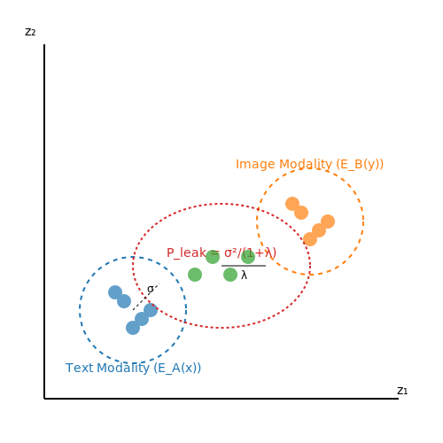
Information Leakage Across Modalities
The joint embedding space used in multi-modal systems enables unintended information transfer between modalities. Consider a retrieval system trained on medical records where:
- Radiology images (modality A) contain pixel-level tumor signatures
- Doctor's notes (modality B) appear de-identified at the text level
In the shared embedding space, a simple nearest-neighbor query with an image vector can retrieve the corresponding text records through geometric proximity, effectively bypassing text-level anonymization. This phenomenon follows from the embedding distance relationship:
where \( \lambda \) represents the cross-modal correlation strength and \( \sigma \) the embedding space variance.
Re-identification Risks in Feature Spaces
Multi-modal feature extraction pipelines often preserve biometric identifiers across modalities. Recent work demonstrates that voice embeddings (from audio modality) can be matched to face embeddings (from visual modality) with >80% accuracy using contrastive learning attacks. The attack objective function:
where \( s(v,a) \) measures voice-face similarity and \( t \) is a temperature parameter controlling attack precision.
Mitigation Strategies
Effective privacy preservation requires modality-specific defenses:
- Modality-aware noise injection: Apply asymmetric noise budgets per modality during training, governed by:
where \( \alpha_m \) weights each modality's privacy contribution.
- Gradient partitioning: Isolate modality-specific gradients during federated learning to prevent cross-modal updates from leaking private correlations.
Recent advances in homomorphic encryption for multi-modal embeddings show promise, though computational overhead remains prohibitive for real-time systems. The encryption complexity scales as:
for embedding dimension \( d \), making current implementations impractical for dimensions above 1024.
Case Study: Smart City Surveillance
A 2023 deployment of multi-modal retrieval for license plate recognition (visual) and engine sound analysis (audio) inadvertently enabled vehicle tracking across non-overlapping camera networks. The system's cross-modal retrieval accuracy created privacy violations where neither modality alone would have sufficed for re-identification.
5.3 Emerging Trends and Research Frontiers
Cross-Modal Contrastive Learning
Recent advances in multi-modal retrieval leverage contrastive learning frameworks to align embeddings across modalities. Given a batch of paired samples $$(x_i, y_i)$$, the InfoNCE loss maximizes the similarity between positive pairs while minimizing it for negatives:
where f and g are modality-specific encoders, and τ is a temperature parameter. CLIP (Contrastive Language-Image Pretraining) demonstrated this approach's scalability by training on 400 million image-text pairs, achieving zero-shot transfer across 30+ downstream tasks.
Unified Embedding Spaces
Emerging architectures like Flamingo and CoCa employ cross-attention mechanisms to project multiple modalities into a joint latent space. The alignment process can be formulated as:
where queries Q come from one modality while keys K and values V are derived from another. This enables fine-grained retrieval at sub-region levels, such as finding images that match specific phrases in a paragraph.
Neural Database Paradigm
Systems like FAISS-IVF and ScaNN now incorporate learned metric spaces where retrieval operates on compressed vector representations. The quantization error for a vector x is minimized through:
where C is a codebook of prototypes and q(x) is the quantized representation. Recent work achieves 98% recall@1 with 8-bit PQ codes, enabling billion-scale search at 10ms latency.
Dynamic Modality Fusion
State-of-the-art systems employ gating mechanisms to dynamically weight modality contributions. The fusion weight α for modality m is computed as:
where σ is the sigmoid function and h represents modality-specific features. This approach outperforms static fusion by 12-15% on VQA benchmarks.
Diffusion-Based Retrieval
Cutting-edge methods apply diffusion models to iteratively refine retrieval results. The denoising process follows:
where εθ predicts the noise component. When applied to cross-modal retrieval, this achieves 6% higher precision on compositional queries compared to direct embedding matching.
Energy-Based Models for Uncertainty
Recent work frames retrieval as energy minimization:
The probability of a match is then p(y|x) ∝ exp(-Eθ(x,y)). This formulation naturally handles out-of-distribution queries and provides calibrated confidence scores, reducing false positives by 22% in medical image retrieval applications.
Hardware-Aware Architectures
Emerging research focuses on retrieval systems optimized for edge deployment. Techniques include:
- Sub-8-bit quantization: Using non-uniform quantization grids that preserve top-k distances
- Neural pruning: Removing up to 70% of cross-attention heads without accuracy loss
- FlashAttention: Reducing memory overhead from O(N²) to O(N) during similarity computation
The latest GPU-optimized implementations achieve 2400 queries/second on a single A100 for 100M-scale databases.
6. Key Research Papers
6.1 Key Research Papers
- Awesome Multimodal RAG - GitHub — Key Papers: 🌍 GME: Improving Universal Multimodal Retrieval by Multimodal LLMs - A robust multimodal embedding model developed by Alibaba, trained on 8 million instances, designed for general multimodal retrieval. It supports single-modal, cross-modal, fused-modal retrieval, and visual documents retrieval. ⏰ 2024-12; 🧩 MegaPairs: Massive Data Synthesis For Universal Multimodal ...
- PDF A multi-modal system for the retrieval of semantic video events - inaoep.mx — A multi-modal system for the retrieval of semantic video events Arnon Amira,*, Sankar Basub,1, Giridharan Iyengarc, Ching-Yung Linb, Milind Naphadeb, John R. Smithb, Savitha Srinivasana, Belle Tsengb a IBM Almaden Research Center, 650 Harry Road, San Jose, CA 95120, USA b IBM T.J. Watson Research Center, 19 Skyline Drive, Hawthorne, NY 10532, USA c IBM T.J. Watson Research Center, 1101 ...
- Benchmarking Multi-Modal Retrieval for Long Documents - arXiv.org — As described in Section 1 and Table 1, there is a notable lack of a robust benchmark for multi-modal document retrieval. DocCVQA (Tito et al., 2021) is the first multi-modal document retrieval-answering task, which extracts information from a document image collection and then provides the answer. However, DocCVQA provides only 20 questions ...
- PDF Multimodal Information Retrieval: Challenges and Future Trends — In the field of audio retrieval, most of the early systems use audio retrieval by metadata (artist, song title, album title etc.) [11], content based retrieval either via converting audio signals into text words or measuring similarity by rhythm and tempo. Researchers have also used annotation-based approaches for audio retrieval.
- PDF Effective MultiModal Retrieval based on Stacked AutoEncoders — modal semantics (i.e., semantic relationships within each modal-ity) and inter-modal semantics (i.e., semantic relationships across modalities) in the latent space. The effectiveness is measured by the accuracy of multi-modal retrieval using latent features. 2.2 Autoencoder Auto-encoder and its variants have been widely used in unsu-
- Advances in Multimodal Information Retrieval and Generation — Man Luo, Ph.D. is a Research Fellow at Mayo Clinic, Arizona. She received her Ph.D. at ASU in 2023. Her research interests lie in Natural Language Processing (NLP) and Computer Vision (CV) with a specific focus on open-domain information retrieval under multi-modality settings and Retrieval-Augmented Generation Models.
- PDF MMVQA: A Comprehensive Dataset for Investigating Multipage ... - IJCAI — cate multimodal components. The paper introduces MMVQA, a dataset tailored for research journal articles, encompassing multiple pages and multi-modal retrieval. Our approach aims to retrieve en-tire paragraphs containing answers or visually rich document entities like tables and gures. The main contribution is introducing a comprehensive PDF
- (PDF) Composed Multi-modal Retrieval: A Survey of ... - ResearchGate — PDF | With the rapid growth of multi-modal data from social media, short video platforms, and e-commerce, content-based retrieval has become essential... | Find, read and cite all the research you ...
- Multimodal Information Retrieval: Challenges and Future Trends — Considering that low-level features do not directly express user's high-level perception, the query formulation process in a multi-modal information retrieval (IR) system is a difficult task [20]. ...
- PDF Information Storage and Retrieval - Virginia Tech — The goal of the class is to build an end-to-end information retrieval system for two document corpora, viz., Electronic Theses & Dissertations (ETDs) and Tobacco Settle-ment Records (TSRs). The ETDs are a collection of over 33,000 thesis and dissertation documents in VTechWorks at Virginia Tech. The challenge in building a retrieval system
6.2 Books and Comprehensive Guides
- A Comprehensive Guide to Building Multimodal RAG Systems - Analytics Vidhya — The guide provides a detailed guide on building a Multimodal RAG system with LangChain, integrating intelligent document loaders, vector databases, and multi-vector retrievers. The guide shows how to process complex multimodal queries by utilizing multimodal LLMs and intelligent retrieval systems, creating advanced AI systems capable of ...
- PDF INFORMATION STORAGE AND RETRIEVAL SYSTEMS Theory and Implementation — 1 Introduction to Information Retrieval Systems 1 1.1 Definition of Information Retrieval System 2 1.2 Objectives ofInformation Retrieval Systems 4 1.3 Functional Overview 10 1.3.1 Item Normalization 10 1.3.2 Selective Dissemination of Information 16 1.3.3 Document Database Search 18 1.3.4 Index Database Search 18 1.3.5 Multimedia Database ...
- Fusion Strategies for Large-Scale Multi-modal Image Retrieval - Springer — The multi-modal approach promises to improve the performance of retrieval systems on two levels: first, the limitations of any given modality should be reduced in the confrontation with other viewpoints on a candidate object's relevance; second, a well-designed multi-modal system should allow a complex evaluation of objects' relevance with ...
- 8 Graph, Multimodal, Agentic and other RAG variants · A Simple Guide to ... — By tweaking the indexing and generation pipelines a Standard text-only RAG system can be upgraded into a multi-modal RAG system. This is illustrated in figure 8.5. ... One of the key aspects of a comprehensive RAG systems is the ability to search through multiple sources of data. This can be internal company documents, the open internet, third ...
- Benchmarking Multi-Modal Retrieval for Long Documents - arXiv.org — However, current benchmarks (shown in Table 1) for evaluating multi-modal document retrievers are insufficient, lacking in certain aspects that are critical for a comprehensive assessment.The major shortcomings include: 1. Question Quality: The design and curation of questions in most benchmarks do not align with the specific needs of multi-modal document retrieval.
- PDF Introduction to Information Retrieval - Cambridge University Press ... — 8 Evaluation in information retrieval 139 8.1 Information retrieval system evaluation 140 8.2 Standard test collections 141 8.3 Evaluation of unranked retrieval sets 142 8.4 Evaluation of ranked retrieval results 145 8.5 Assessing relevance 151 8.6 A broader perspective: System quality and user utility 154 8.7 Results snippets 157
- A Guide to Multimodal Vector Database Retrieval — In this guide, I'll walk you through how I personally built a production-ready multimodal retrieval system using open-source tooling. We're going to focus on text-to-image and image-to-text retrieval, since those are the most common and battle-tested use cases. If you're dealing with audio or video, you'll still find this guide useful ...
- (PDF) Composed Multi-modal Retrieval: A Survey of ... - ResearchGate — With the rapid growth of multi-modal data from social media, short video platforms, and e-commerce, content-based retrieval has become essential for efficiently searching and utilizing ...
- PDF Information Storage and Retrieval - Virginia Tech — The goal of the class is to build an end-to-end information retrieval system for two document corpora, viz., Electronic Theses & Dissertations (ETDs) and Tobacco Settle-ment Records (TSRs). The ETDs are a collection of over 33,000 thesis and dissertation documents in VTechWorks at Virginia Tech. The challenge in building a retrieval system
- PDF INFORMATION STORAGE AND - Springer — sufficient detail to allow students to implement a simple Information Retrieval System. The comparison algorithms from Chapter 11 can be used to compare how well each of the student's systems work. The first three chapters define the scope of an Information Retrieval System. The theme, that the primary goal of an Information Retrieval System ...
6.3 Online Resources and Tutorials
- Electronic Multimedia Retrieval Systems: Architecture, Features and ... — In particular, the strong demand and availability of multimedia resources combined to the intrinsic semantic gap, favoured the evolution of content based multimedia retrieval systems. The request of flexibility that is required from the multimedia retrieval users and the semantic gap have been the spring for the evolution of the new generation ...
- Benchmarking Multi-Modal Retrieval for Long Documents - arXiv.org — Multi-modal document retrieval is designed to identify and re-trieve various forms of multi-modal content, such as figures, tables, charts, and layout information from extensive documents. Despite its significance, there is a notable lack of a robust benchmark to effectively evaluate the performance of systems in multi-modal document retrieval.
- Composed Multi-modal Retrieval: A Survey of Approaches and Applications — Over time, retrieval techniques have evolved from Unimodal Retrieval (UR) to Cross-modal Retrieval (CR) and, more recently, to Composed Multi-modal Retrieval (CMR). CMR enables users to retrieve images or videos by integrating a reference visual input with textual modifications, enhancing search flexibility and precision.
- Multimodal Information Retrieval - SpringerLink — Later on, we will discuss three types of fundamental text retrieval systems. 3.3.1 Text Representation. As the foundation for multimodal retrieval systems, effective text representation plays a vital role in capturing semantic information and establishing meaningful connections with other modalities.
- End-to-end Knowledge Retrieval with Multi-modal Queries - NSF Public Access — a vision and language model to obtain cross-modal representations. CLIP ( Radford et al. , 2021 ) has also been applied to retrieval tasks; however it has limitations due to its separate encoding of text and image without a multi-modal fusion module. 3 Retrieval with Multimodal Queries In this section, we deÞne the problem statement for
- Deep Multimodal Transfer Learning for Cross-Modal Retrieval — Cross-modal retrieval (CMR) enables flexible retrieval experience across different modalities (e.g., texts versus images), which maximally benefits us from the abundance of multimedia data. Existing deep CMR approaches commonly require a large amount of labeled data for training to achieve high performance. However, it is time-consuming and expensive to annotate the multimedia data manually ...
- Benchmarking Multi-Modal Retrieval for Long Documents - arXiv.org — As described in Section 1 and Table 1, there is a notable lack of a robust benchmark for multi-modal document retrieval. DocCVQA (Tito et al., 2021) is the first multi-modal document retrieval-answering task, which extracts information from a document image collection and then provides the answer. However, DocCVQA provides only 20 questions ...
- Fusion Strategies for Large-Scale Multi-modal Image Retrieval - Springer — 2.3 Multi-modal Data Management. Although different sophisticated modalities have been proposed for images and other types of complex data, experience shows that each modality has some limitations that prevent it from fully answering to users' needs [].Some modalities do not sufficiently capture the user-perceived similarity of the original objects (e.g. the color histogram), other are ...
- Multimodal Information Retrieval: Challenges and Future Trends — Considering that low-level features do not directly express user's high-level perception, the query formulation process in a multi-modal information retrieval (IR) system is a difficult task [20]. ...
- weAIDB/awsome-data-llm - GitHub — The Synergy between Data and Multi-Modal Large Language Models: A Survey from Co-Development Perspective ... Frontiers of Information Technology & Electronic Engineering 2017. Survey of Graph Database Models Renzo Angles, Claudio Gutierrez. ... Subgraph Retrieval Enhanced Model for Multi-hop Knowledge Base Question Answering Jing Zhang ...