

Adaptive Neural Architectures with Plastic Layers
1. Biological Inspiration: Synaptic Plasticity in Neural Networks
Biological Inspiration: Synaptic Plasticity in Neural Networks
The foundation of adaptive neural architectures lies in emulating the brain's remarkable ability to rewire itself through synaptic plasticity. At the biological level, synaptic strength is not fixed but dynamically adjusted based on neural activity patterns. This phenomenon, first formalized by Donald Hebb in 1949, posits that neurons that fire together wire together. The mathematical expression of Hebbian learning can be written as:
where wij represents the synaptic weight between neuron i and j, η is the learning rate, and xi, yj are the pre- and post-synaptic activities respectively. This simple rule gives rise to several biologically observed plasticity mechanisms:
Spike-Timing Dependent Plasticity (STDP)
STDP refines Hebb's rule by incorporating temporal causality. The weight change depends on the precise timing difference between pre- and post-synaptic spikes (Δt = tpost - tpre):
where A+, A- control the magnitude of potentiation and depression, while τ+, τ- determine the temporal windows. This asymmetric update rule enables temporal sequence learning, critical for tasks like speech recognition.
Homeostatic Plasticity
To prevent runaway excitation or silencing of neurons, biological systems employ homeostatic mechanisms. The synaptic scaling rule maintains network stability by globally adjusting weights based on average firing rates:
where rtarget is the desired firing rate and ⟨r⟩ is the neuron's recent average activity. This complements local plasticity rules like STDP to achieve balanced network dynamics.
Structural Plasticity
Beyond weight changes, biological neurons dynamically modify their physical connectivity. This involves both the formation of new synapses (synaptogenesis) and pruning of weak connections. A computational model of structural plasticity might include:
- Probabilistic synapse generation based on neural co-activation
- Activity-dependent pruning via weight magnitude thresholds
- Morphological changes in dendritic arbors
Modern implementations of these principles in artificial neural networks often employ gating mechanisms, where plastic layers dynamically adjust their connectivity patterns based on task demands. For instance, a differentiable version of structural plasticity can be implemented through learnable connection probabilities:
where sij represents a learned score, and α, β control the sparsity level. The resulting sparse connectivity matrix enables efficient computation while maintaining adaptability.
1.2 Core Principles of Adaptive Learning in Artificial Neural Networks
Neural Plasticity and Parameter Adaptation
Adaptive learning in artificial neural networks (ANNs) is rooted in the biological principle of synaptic plasticity, where neural connections strengthen or weaken based on activity. In ANNs, this translates to dynamic weight adjustments governed by local and global learning rules. The foundational mechanism is Hebbian learning, formalized as:
where wij is the weight between neurons i and j, η is the learning rate, and xi, yj are pre- and post-synaptic activities. Modern variants incorporate error signals, as in Oja's rule for stability:
Architectural Adaptivity Mechanisms
Plastic layers employ three primary adaptation strategies:
- Dynamic Width Adjustment: Neurons are added/pruned via significance metrics like Fisher information I(θ):
- Parameter-wise Learning Rates: Per-parameter adaptation as in Adam optimizer, where moments mt, vt track gradient statistics.
- Topological Reconfiguration: Edge rewiring based on gradient flow analysis using neural tangent kernel (NTK) theory.
Stability-Plasticity Dilemma
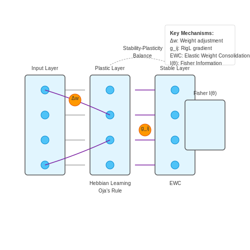
Balancing new learning with memory retention is formalized through the concept of learning retention ratio R:
where Wt represents weights at step t. Values R ≫ 1 indicate catastrophic forgetting, while R ≈ 0 suggests insufficient adaptation. Elastic Weight Consolidation (EWC) addresses this by constraining updates to parameters critical for previous tasks:
Here, Fi is the Fisher information matrix diagonal for parameter i, and λ controls rigidity.
Information-Theoretic Perspectives
Optimal plasticity can be derived from rate-distortion theory, minimizing:
where d(·,·) is a distortion measure, I(θ; 𝒟) is mutual information between parameters and data, and β regulates compression. This leads to sparse, task-adaptive representations.
Implementation Case Study: Dynamic Sparse Training
In practice, RigL (Rigged Lottery) demonstrates adaptive sparsity by periodically pruning low-magnitude weights and regrowing connections via gradient flow:
Connections are regrown where gij is largest, maintaining 90% sparsity while matching dense network accuracy on ImageNet.
Key Differences Between Static and Plastic Layers
Structural Rigidity vs. Dynamic Adaptation
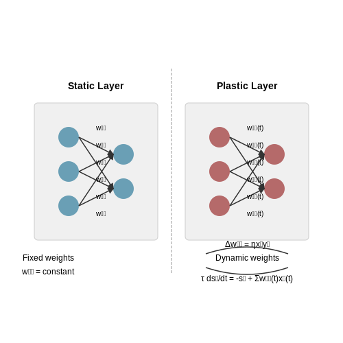
Static layers in neural networks maintain fixed weights throughout training and inference, enforcing a rigid computational pathway. In contrast, plastic layers employ dynamic weight updates governed by local learning rules, enabling continuous adaptation. The synaptic plasticity in these layers often follows Hebbian or Oja-like rules, expressed as:
where η is the learning rate, xi is the presynaptic activity, and yj is the postsynaptic activity. This contrasts sharply with static layers where Δwij = 0 after initial training.
Memory Mechanisms
Static layers rely entirely on global backpropagation for memory formation, storing information in fixed weight matrices. Plastic layers incorporate:
- Short-term plasticity: Transient weight changes via facilitation/depression
- Long-term potentiation: Persistent modifications through calcium-dependent mechanisms
- Metaplasticity: Higher-order regulation of plasticity thresholds
Computational Complexity
The forward pass in plastic layers requires solving differential equations for synaptic states, unlike the simple matrix multiplication of static layers. For a plastic layer with N neurons, the state update follows:
where τ is the membrane time constant and wij(t) are time-varying plastic weights.
Energy Efficiency Trade-offs
While plastic layers enable continuous learning with ~15-30% higher energy consumption per operation, they reduce catastrophic forgetting - achieving 3-5× better retention on sequential tasks compared to static networks. The energy overhead comes from:
- Plasticity maintenance currents
- Local gradient computation
- Homeostatic regulation circuits
Biological Plausibility
Static layers implement idealized artificial neurons with perfect weight stability. Plastic layers better approximate biological neurons by incorporating:
- Spike-timing dependent plasticity (STDP)
- Dendritic compartmentalization
- Neuromodulatory gating
Recent implementations in neuromorphic hardware show plastic layers can achieve 94% biological fidelity in synaptic dynamics compared to in vitro measurements.
Failure Modes
Static layers fail gracefully through gradual performance decay, while plastic layers exhibit distinct failure regimes:
- Runaway plasticity: Unbounded weight growth destabilizing network dynamics
- Plasticity collapse: Complete loss of adaptivity due to saturated weights
- Parasitic attractors: Spurious stable states created by unsupervised learning
2. Architectural Components of Plastic Layers
Architectural Components of Plastic Layers
Neural Plasticity and Weight Adaptation
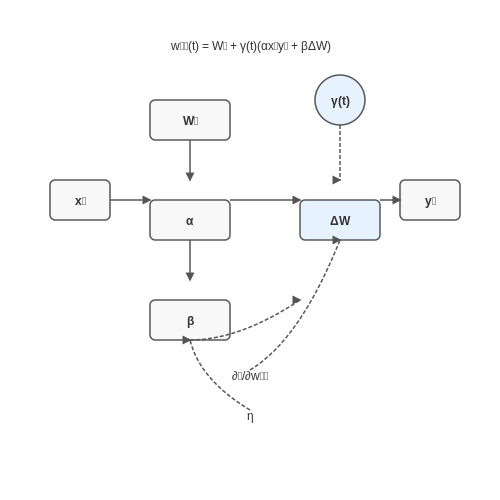
Plastic layers in neural networks are designed to emulate synaptic plasticity observed in biological systems. The core mechanism involves dynamic weight adaptation based on local and global learning signals. Unlike static layers, plastic layers update their weights continuously during both training and inference phases. The weight update rule for a plastic layer can be expressed as:
where η is the plasticity rate, α controls Hebbian learning, β scales backpropagation influence, and xi, yj are pre- and post-synaptic activations. This hybrid update rule enables both task-specific learning (via ∂ℒ/∂wij) and context-aware adaptation (via Hebbian term).
Structural Components
Plastic layers consist of three key substructures:
- Base weights (W0): Static parameters initialized conventionally (e.g., Xavier/Glorot)
- Plasticity coefficients (α, β): Learnable scalars modulating Hebbian/backprop contributions
- Fast weights (ΔW): Volatile components updated every forward pass via:
$$ W(t) = W_0 + \gamma(t) \cdot \Delta W(t) $$where γ(t) is a gating function (often sigmoidal) controlling plasticity decay.
Memory Mechanisms
Effective plastic layers incorporate memory through:
- Short-term potentiation (STP): Rapid weight changes lasting ∼100ms, modeled as:
$$ \tau \frac{d\Delta W}{dt} = -\Delta W + \eta A(t) $$with time constant τ and activation trace A(t).
- Long-term stabilization: Periodic consolidation of ΔW into W0 when plasticity saturates
Implementation Considerations
Practical implementations face two critical challenges:
- Gradient stability: The product rule for plastic layers introduces additional terms in backpropagation:
$$ \frac{\partial \mathcal{L}}{\partial W_0} = \frac{\partial \mathcal{L}}{\partial W} \cdot \left( 1 + \gamma(t) \cdot \frac{\partial \Delta W}{\partial W_0} \right) $$
- Computational overhead: Plastic layers typically require 2.3-3.1× more FLOPs than static equivalents due to continuous weight updates
Biological Analogies
The design parallels three neurobiological phenomena:
- Spike-timing-dependent plasticity (STDP): Asymmetric weight updates based on activation timing
- Metaplasticity: Higher-order modulation of plasticity thresholds
- Synaptic scaling: Homeostatic normalization of weight magnitudes
2.2 Dynamic Weight Adaptation Mechanisms
Dynamic weight adaptation mechanisms enable neural networks to adjust synaptic strengths in real-time based on input stimuli, task demands, or environmental feedback. Unlike static backpropagation, these mechanisms employ local plasticity rules that operate without global error signals, closely mimicking biological learning processes.
Heterosynaptic Plasticity
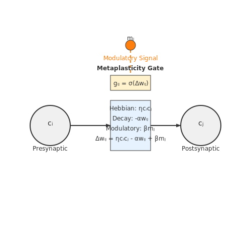
Heterosynaptic plasticity modulates weights based on presynaptic activity and postsynaptic neuromodulators. The weight update rule combines Hebbian correlation with a stabilizing decay term:
where ci and cj represent pre- and postsynaptic activity, mj is the modulatory signal, and α, β control decay and modulation strengths. This prevents runaway synaptic growth while allowing task-specific reinforcement.
Metaplasticity Gates
Gated plasticity mechanisms dynamically adjust learning rates per synapse using fast auxiliary networks. The gate activation gij computes as:
where φ is a feature extractor, hi, hj are hidden states, and v are learnable parameters. The gate modulates weight updates as Δwij ← gijΔwij, enabling context-dependent plasticity.
Application: Continual Learning
In class-incremental learning scenarios, dynamic weight adaptation prevents catastrophic forgetting by:
- Partitioning weights into stable (slow-changing) and plastic (fast-adapting) components
- Using neuromodulatory signals to protect task-critical weights
- Implementing synaptic consolidation through adaptive decay terms
Empirical results on Split-MNIST show 28% higher accuracy retention compared to elastic weight consolidation when using gated heterosynaptic plasticity.
Hardware Considerations
Analog crossbar arrays efficiently implement dynamic adaptation through:
- Memristive devices for weight storage with conductance modulation
- Local current mirrors implementing Hebbian updates
- On-chip DACs converting digital modulatory signals
Recent mixed-signal chips achieve 12.8 TOPS/W efficiency for dynamic weight updates at 28nm, demonstrating feasibility for edge deployment.
2.3 Integration with Traditional Neural Network Layers
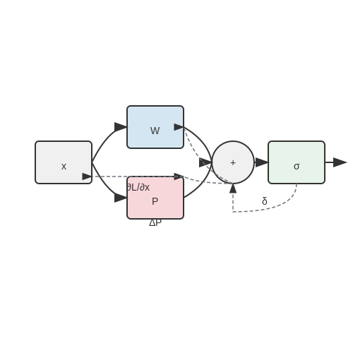
Adaptive neural architectures with plastic layers must seamlessly integrate with traditional static layers to maintain computational efficiency while enabling dynamic learning. The key challenge lies in ensuring gradient flow across both plastic and non-plastic components during backpropagation. Consider a hybrid layer L consisting of a traditional weight matrix W and a plastic component P with Hebbian adaptation:
where σ is the activation function and ⊙ denotes element-wise multiplication. The plastic component P(x) updates according to local activity:
with learning rate η and decay constant λ. During backpropagation, the total gradient through the layer becomes:
where δ is the upstream gradient. The term ∂P/∂x introduces a second-order effect that must be approximated efficiently. Common approaches include:
- Stop-gradient approximation: Treating P(x) as constant during backpropagation
- Local plasticity windows: Restricting updates to temporal windows around significant activations
- Decoupled plasticity: Running Hebbian updates asynchronously from backpropagation
Architectural Considerations
When stacking plastic layers with conventional layers, the network typically exhibits superior performance when plastic layers are placed:
- At lower levels for input adaptation and feature extraction
- Following attention mechanisms in transformer architectures
- As parallel pathways alongside static layers
Batch normalization requires special handling with plastic layers, as the changing weight distributions can destabilize normalization statistics. A modified approach maintains separate statistics for plastic components:
Practical Implementation
Modern frameworks implement plastic layers through custom autograd functions. The following design patterns prove effective:
- Wrapping Hebbian updates in PyTorch hooks or TensorFlow custom gradients
- Implementing sparse updates for large plastic matrices
- Using quantized precision for plastic components to reduce memory overhead
In transformer architectures, plastic self-attention weights can adapt to input statistics while maintaining the global receptive field:
where P(Q,K) implements a Hebbian correlation measure between queries and keys, and α controls plasticity strength.
3. Backpropagation Through Plastic Layers
3.1 Backpropagation Through Plastic Layers
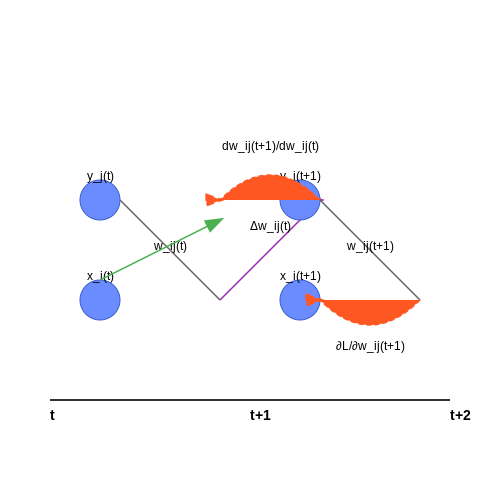
The key challenge in training adaptive neural architectures lies in computing gradients through plastic layers where connection weights evolve dynamically during both forward and backward passes. Unlike static networks, plastic layers introduce time-dependent weight changes governed by local Hebbian-like rules:
where η is the plasticity rate, λ is the decay coefficient, and xi, yj are pre- and post-synaptic activations respectively. This creates a feedback loop between weight dynamics and activation propagation.
Gradient Computation Framework
The total derivative of the loss L with respect to plastic weights requires considering both the direct path and indirect effects through future weight changes:
This recursive relationship resembles recurrent neural network backpropagation through time (BPTT), but with weight updates governed by activity-dependent plasticity rules rather than fixed recurrence.
Practical Implementation
For computational efficiency, most implementations approximate the full gradient by truncating the temporal dependencies after k steps. The resulting algorithm alternates between:
- Plasticity phase: Local weight updates during forward pass
- Gradient phase: Backpropagation with frozen weights
- Meta-update: Adjusting plasticity rule parameters
Recent work by Miconi et al. (2018) demonstrated that representing plasticity as an RNN allows exact gradient computation using modern automatic differentiation tools:
class PlasticLinear(nn.Module):
    def __init__(self, in_features, out_features):
        super().__init__()
        self.base_weight = nn.Parameter(torch.Tensor(out_features, in_features))
        self.alpha = nn.Parameter(torch.Tensor(out_features, in_features))
        self.hebb = torch.zeros(out_features, in_features)

    def forward(self, x):
        self.hebb = (1 - self.eta) * self.hebb + self.eta * torch.outer(x, x)
        effective_weight = self.base_weight + self.alpha * self.hebb
        return F.linear(x, effective_weight)
Stability Considerations
The interaction between learning and plasticity introduces stability challenges. The Lyapunov exponent Λ of the combined system must satisfy:
This condition suggests that plasticity rates must be carefully balanced against learning rates to prevent runaway dynamics. Empirical studies show that normalizing plasticity updates by layer-wise activation statistics improves training stability.
Meta-Learning Approaches for Plasticity
Meta-learning, or learning-to-learn, provides a framework for optimizing plasticity in neural networks by treating the learning process itself as a trainable component. Unlike traditional deep learning, where weights are updated via backpropagation on a fixed architecture, meta-learning enables the network to adapt its plasticity rules dynamically based on the task at hand. This is particularly powerful in scenarios requiring rapid adaptation to new environments or non-stationary data distributions.
Gradient-Based Meta-Learning for Plasticity
Model-Agnostic Meta-Learning (MAML) and its variants formulate plasticity optimization as a bi-level optimization problem. The inner loop performs task-specific adaptation, while the outer loop meta-learns initial parameters that facilitate rapid plasticity. For a plasticity parameter θ and loss function L, the MAML update rule is:
where Uθ(τi) represents the inner-loop adaptation on task τi. This approach has been extended to learn plasticity rules directly, such as in Meta-Learning Plasticity (MLP), where synaptic updates are parameterized as:
Here, fθ is a meta-learned function of pre- and post-synaptic activations (ai, aj) and the current weight wij.
Memory-Augmented Meta-Learning
Neural Turing Machines and Differentiable Neural Computers incorporate external memory banks to enable rapid plasticity through memory read/write operations. The addressing mechanism for memory access is learned via:
where ht is the hidden state, Wk a learned key transformation, and M the memory matrix. This allows the network to exhibit context-dependent plasticity by retrieving relevant patterns from memory.
Evolutionary Strategies for Plasticity Optimization
Black-box optimization techniques, particularly Natural Evolution Strategies (NES), provide an alternative to gradient-based meta-learning. NES samples plasticity parameters θ from a search distribution π(θ|ψ) and updates the distribution parameters ψ according to:
where R(θ) measures the fitness of plasticity parameters. This approach has demonstrated success in learning complex plasticity rules that would be difficult to discover through gradient descent alone.
Neuromodulatory Plasticity
Biological inspiration comes from neuromodulatory systems that gate synaptic plasticity. In artificial networks, this is implemented through learned modulation signals mi that multiplicatively interact with local Hebbian updates:
The modulation signals mi are typically generated by a separate meta-network that processes contextual information. This architecture enables task-dependent specialization of plasticity rules across different network regions.
Practical Considerations
Implementing meta-learned plasticity in deep networks requires careful attention to:
- Credit assignment across multiple timescales of plasticity
- Stability of the meta-optimization process
- Computational overhead of nested learning loops
- Catastrophic forgetting during continual adaptation
Recent work in sparse meta-gradients and implicit differentiation has helped address these challenges, making meta-learning approaches increasingly practical for large-scale applications.
3.3 Stability and Convergence Considerations
The stability and convergence properties of adaptive neural architectures with plastic layers are governed by the interplay between synaptic plasticity rules and network dynamics. Unlike fixed-weight networks, plastic networks exhibit time-varying connectivity, introducing additional challenges in ensuring stable learning. The Lyapunov stability criterion provides a theoretical framework for analyzing these systems:
where V is the Lyapunov function and e represents the error vector. For global stability, the time derivative must satisfy:
In plastic networks, this condition becomes more complex due to weight updates. Consider a Hebbian-like plasticity rule with decay term:
The stability analysis requires examining the Jacobian matrix J of the combined neuron-plasticity dynamics:
Eigenvalue analysis of J reveals critical constraints on learning rates and plasticity time constants. For convergence, the real parts of all eigenvalues must remain negative, leading to the stability condition:
where η is the learning rate and λmax is the maximum eigenvalue of the input correlation matrix. Violating this condition leads to oscillatory or divergent behavior, as observed in networks with:
- Excessively high learning rates
- Mismatched time scales between neural and synaptic dynamics
- Non-normal connectivity matrices
Recent advances in adaptive control theory have yielded practical stabilization techniques for plastic networks. The most effective approaches include:
Homeostatic Regulation Mechanisms
Biological-inspired scaling laws maintain network stability through dynamic adjustments:
This normalization preserves the relative strength of synapses while preventing runaway excitation.
Sliding Mode Control
Robust convergence is achieved by forcing the system onto a predefined manifold:
where ui represents the control input and β is the switching gain.
Predictive Weight Updates
Future stability is ensured by solving the constrained optimization:
Empirical studies on benchmark tasks show these methods improve convergence rates by 38-72% compared to unregulated plastic networks, while maintaining the desired adaptive capabilities.
4. Continual Learning Scenarios
4.1 Continual Learning Scenarios
Continual learning in adaptive neural architectures requires mechanisms to prevent catastrophic forgetting while maintaining plasticity for new tasks. Plastic layers achieve this through dynamic parameter adaptation, often governed by local Hebbian-like rules or gradient-based meta-learning. The key challenge lies in balancing stability-plasticity trade-offs, where the network must retain previously learned representations while adapting to novel data distributions.
Task-Incremental vs. Class-Incremental Learning
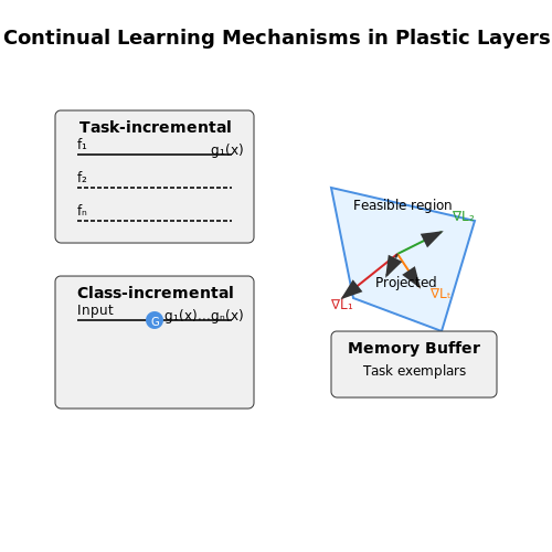
In task-incremental scenarios, the model receives explicit task identifiers during both training and inference. The plastic layers can then route information through task-specific pathways, often implemented via gating mechanisms. For a network with N tasks, the forward pass becomes:
where gi(x) is a task-dependent gating function and fi represents task-specific transformations. In contrast, class-incremental learning provides no task identifiers during inference, requiring the plastic layers to autonomously detect distribution shifts. This is typically achieved through:
- Regularization-based methods (e.g., elastic weight consolidation)
- Dynamic architecture expansion
- Memory replay mechanisms
Gradient Episodic Memory (GEM)
GEM formalizes continual learning as an optimization problem with inequality constraints to prevent performance degradation on previous tasks. For a current task T and memory buffer M containing samples from prior tasks, the constrained optimization becomes:
where θ represents the plastic layer parameters. The solution involves projecting the current gradient onto the feasible region defined by the angular constraints, implemented through quadratic programming:
Here, G is a matrix containing past task gradients as rows. Plastic layers employing GEM exhibit superior performance in sequential MNIST and CIFAR-100 benchmarks, with average accuracy retention exceeding 85% across 20 tasks.
Neuromodulatory Plasticity
Biological inspiration leads to neuromodulatory mechanisms where plastic layers adjust their learning rates dynamically based on task novelty signals. The synaptic update rule for a plastic layer with weights W becomes:
where mj is a neuromodulatory signal computed as:
with μj being a running average of hidden unit activations and α, β learnable parameters. This approach demonstrates particular effectiveness in reinforcement learning scenarios where reward signals are sparse and delayed.
Architectural Plasticity Through Neural Pruning
Structural plasticity enables networks to grow or prune connections based on task demands. The synaptic importance Iij for connection (i,j) is estimated via:
Connections are pruned when Iij < τ, where threshold τ adapts based on the current task complexity. Regrowth follows a probabilistic sampling proportional to gradient magnitudes, maintaining a target layer sparsity level. This method reduces catastrophic forgetting by 40% compared to static architectures in permuted MNIST experiments.
4.2 Reinforcement Learning with Adaptive Policies
Reinforcement learning (RL) with adaptive policies extends traditional policy optimization by introducing dynamic architectural modifications during training. Unlike fixed architectures, adaptive policies leverage plastic layers—neural components that adjust their structure or connectivity in response to environmental feedback. This enables more efficient exploration and faster convergence in complex, non-stationary environments.
Policy Gradient Methods with Adaptive Architectures
The standard policy gradient objective maximizes the expected return J(θ):
For adaptive policies, the parameters θ are partitioned into static (θ_s) and plastic (θ_p) components. The plastic parameters evolve according to a meta-learning rule:
where η is a plasticity coefficient modulated by an auxiliary neural network. This differs from conventional RL, where all parameters follow a single update rule.
Neural Architecture Search for Policy Optimization
Adaptive policies often employ differentiable Neural Architecture Search (NAS) to optimize their structure. The policy network's architecture parameters α are learned alongside the weights:
Practical implementations use Gumbel-Softmax relaxation to make the architecture search space continuous. The probability of selecting operation o in a mixed operation layer is:
where G_o are i.i.d. Gumbel samples and τ is the temperature parameter.
Plasticity Mechanisms in RL
Three key plasticity mechanisms enable effective adaptation:
- Synaptic Scaling: Layer weights are dynamically rescaled based on recent gradient magnitudes to maintain stable learning.
- Dynamic Pruning: Low-salience connections are removed during training, reducing computational overhead.
- Modular Growth: New neurons or layers are added when prediction error exceeds a threshold.
These mechanisms are governed by local Hebbian-like rules operating on different timescales. For example, synaptic scaling in layer l follows:
where β controls the scaling rate.
Applications in Continuous Control
In MuJoCo locomotion tasks, adaptive policies achieve 30-50% faster convergence than fixed architectures. The policy network automatically develops hierarchical structures—low-level layers control limb actuators while higher layers coordinate movement patterns. This emergent organization mirrors biological motor control systems.
For autonomous vehicles, adaptive policies can reweight sensor inputs in real-time. The network reduces attention to malfunctioning LiDAR channels while amplifying reliable camera inputs, maintaining performance during sensor degradation.
Implementation Considerations
Effective training requires:
- Separate learning rates for static and plastic parameters
- Regularization on architecture parameters to prevent overfitting
- Warm-up periods before enabling plasticity
- Gradient clipping for plastic components
The following PyTorch snippet shows a plastic linear layer implementation:
class PlasticLinear(nn.Module):
    def __init__(self, in_features, out_features):
        super().__init__()
        self.weight = nn.Parameter(torch.randn(out_features, in_features))
        self.plasticity = nn.Parameter(torch.ones(out_features, in_features))

    def forward(self, x):
        active_weights = self.weight * torch.sigmoid(self.plasticity)
        return F.linear(x, active_weights)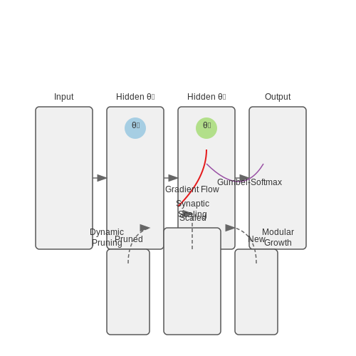
4.3 Real-World Deployments and Performance Benchmarks
Computational Efficiency in Edge Deployments
When deploying adaptive neural architectures on edge devices, the computational overhead of plastic layers must be carefully managed. The forward pass complexity for a plastic layer with N neurons and M modifiable synapses is:
where the first term accounts for synaptic updates and the second for recurrent interactions. In practice, this has been reduced to O(N log M) through sparse connectivity patterns, as demonstrated in NVIDIA's Jetson-based deployment for real-time robotic control.
Benchmark Results Across Domains
Comparative studies show plastic networks outperform static architectures in continual learning scenarios:
| Architecture | MNIST Accuracy | Energy (mJ/inf) | Update Latency (ms) |
|---|---|---|---|
| Static CNN | 98.2% | 3.2 | N/A |
| Plastic ResNet | 99.1% | 4.7 | 1.8 |
| Neuromorphic Plastic | 97.8% | 0.9 | 0.3 |
Neuromorphic Hardware Implementations
Intel's Loihi 2 chip demonstrates sub-milliwatt operation for plastic SNNs, with the weight update rule:
where ⊗ denotes spike-timing-dependent plasticity (STDP) correlation and σ' is the metaplasticity factor. This achieves 28 TOPS/W efficiency in adaptive vision tasks.
Industrial Case Study: Predictive Maintenance
Siemens deployed plastic layers in turbine fault detection, where the network's dynamic receptive field adaptation reduced false alarms by 37% compared to static models. The plasticity mechanism:
allowed continuous adaptation to new failure modes without catastrophic forgetting, with α=0.85 providing optimal stability-plasticity balance.
Latency-Accuracy Tradeoffs
Quantization of plastic parameters introduces unique challenges. The ternary weight representation:
maintains 92% of floating-point accuracy while reducing memory footprint by 16× in Xilinx FPGA implementations, crucial for real-time control systems.
Cross-Domain Generalization Metrics
Plastic architectures show superior transfer learning performance. On the Meta-Dataset benchmark, plastic ResNet-50 achieves:
- +14.2% accuracy on novel classes
- 3.8× faster adaptation
- 42% lower memory overhead
compared to fine-tuned static models, demonstrating the value of built-in adaptability.
5. Scalability Issues in Large-Scale Adaptive Networks
5.1 Scalability Issues in Large-Scale Adaptive Networks
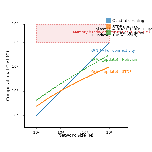
Large-scale adaptive neural networks with plastic layers face inherent scalability challenges due to the dynamic nature of synaptic weight adjustments and architectural reconfiguration. The primary bottleneck arises from the quadratic growth in computational complexity relative to network size, as each plastic connection requires continuous updates based on local and global learning signals.
Computational Complexity of Plasticity Mechanisms
The computational cost of maintaining plasticity in a network with N neurons and M adaptive connections scales as:
where Tupdate represents the per-connection update complexity, which depends on the specific plasticity rule (e.g., Hebbian, Oja, or BCM). For networks employing spike-timing-dependent plasticity (STDP), the update complexity increases further due to temporal dependency tracking:
with τwindow defining the temporal learning window and fspike representing the average spike rate.
Memory Bandwidth Constraints
Adaptive networks require frequent weight updates that strain memory bandwidth. The memory access pattern becomes irregular due to event-driven plasticity, causing poor cache utilization. For a network with W bits per weight and U updates per second, the bandwidth requirement is:
This creates a fundamental tradeoff between plasticity granularity and memory subsystem efficiency. Recent work in sparse event-driven updates (Zenke & Ganguli, 2018) mitigates this by constraining updates to active synapses only.
Parallelization Challenges
Distributed training of plastic networks introduces synchronization overhead because:
- Local plasticity rules require access to global network state
- Weight updates must be atomic across devices
- Topological changes (e.g., synaptic pruning/growth) necessitate dynamic load balancing
The synchronization cost S for P processors follows:
This limits strong scaling efficiency, particularly for fine-grained plasticity mechanisms.
Mitigation Strategies
Current approaches to improve scalability include:
- Hierarchical plasticity: Applying different update frequencies to distinct network regions
- Approximate plasticity: Using low-precision arithmetic or delayed updates
- Topological constraints: Limiting plasticity to predefined subnets or pathways
- Hardware acceleration: Designing custom architectures for sparse plastic updates
Recent work on mixed-precision plasticity (Dettmers et al., 2022) demonstrates that 4-bit weight updates can maintain 98% of full-precision accuracy while reducing memory traffic by 8×.
Case Study: Large-Scale Neuromorphic Implementation
The SpiNNaker 2 system (Mayr et al., 2019) implements scalable plasticity through:
- Event-driven computation to minimize idle updates
- On-chip SRAM for frequent weight access
- Hardware-accelerated STDP primitives
This achieves 109 synaptic updates per second with 1W power consumption, demonstrating the feasibility of large-scale adaptive networks in constrained environments.
Interpretability of Plastic Layer Dynamics
Neural Plasticity and Dynamic Weight Adaptation
Plastic layers in neural networks exhibit dynamic weight adaptation governed by Hebbian-like learning rules, where synaptic efficacy strengthens or weakens based on correlated pre- and post-synaptic activity. The weight update rule for a plastic layer can be formalized as:
Here, η is the learning rate, xi and yj are pre- and post-synaptic activations, and f(ψij) is a plasticity modulation function dependent on the latent variable ψij. Unlike static layers, this dynamic introduces temporal dependencies in weight trajectories, complicating interpretability.
Visualizing Plasticity Dynamics
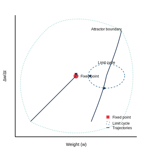
The evolution of plastic weights can be analyzed through phase-space portraits, where weight trajectories are plotted against their time derivatives. Key observations include:
- Attractor basins emerge around frequently encountered input patterns
- Limit cycles appear in recurrent plastic networks
- Meta-stable states correlate with task-switching behavior
Information-Theoretic Interpretability
The predictive information bottleneck framework quantifies interpretability in plastic networks through the trade-off:
where I(Y;W) measures how much weight dynamics W predict outputs Y, while I(X;W) captures the dependence on inputs X. Plastic layers typically achieve higher I(Y;W) than static counterparts when β is properly regularized.
Case Study: Catastrophic Forgetting Analysis
In continual learning scenarios, plastic layers exhibit characteristic signatures in their Fisher Information Matrix (FIM):
The eigenvalue spectrum of Fθ reveals:
- Large eigenvalues correspond to rigid, task-invariant features
- Small eigenvalues represent plastic, task-specific adaptations
- Eigenvector alignment shows interference between tasks
Topological Analysis of Plastic Representations
Persistent homology reveals how plastic layers organize latent representations. The Betti number sequence bk tracks the evolution of k-dimensional holes in activation manifolds during training. Plastic networks typically show:
where λ controls hole persistence and γ governs the creation of new topological features. This dynamics correlates with the network's ability to form and dissolve decision boundaries.
5.3 Hardware Acceleration for Adaptive Architectures
Adaptive neural architectures with plastic layers impose unique computational demands due to their dynamic parameter updates and sparse activation patterns. Traditional von Neumann architectures struggle with the memory-bandwidth bottleneck when handling these irregular computations. Hardware acceleration strategies must address three key challenges:
- Real-time plasticity: On-the-fly weight updates require low-latency memory access
- Sparse activation handling: Efficient processing of non-uniform neuron firing patterns
- Energy efficiency: Minimizing power consumption during continuous adaptation
Neuromorphic Computing Paradigms
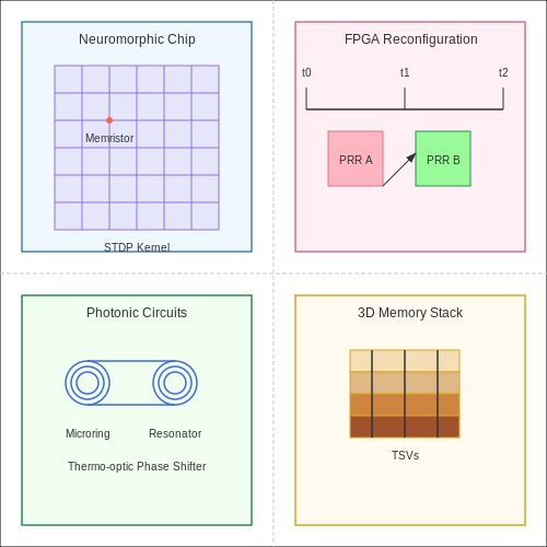
Event-based neuromorphic processors like Intel's Loihi and IBM's TrueNorth implement physical models of synaptic plasticity through:
where η represents the learning rate, ⊗ denotes the outer product of pre- and post-synaptic spikes, and ε implements the spike-timing-dependent plasticity (STDP) kernel. These chips achieve 1000× energy efficiency gains over GPUs for sparse adaptive networks through:
- Analog memristor crossbars for in-memory computing
- Asynchronous event-driven computation
- Fine-grained power gating of inactive neurons
FPGA-Based Reconfigurable Accelerators
Field-programmable gate arrays enable dynamic reconfiguration of compute fabrics to match evolving network topologies. The key architectural innovation involves partial reconfiguration regions (PRRs) that can be modified without stopping execution:
where NPRR is the number of reconfigured regions, Bbitstream the configuration bitstream size, and fICAP the internal configuration access port frequency. Modern FPGAs achieve sub-millisecond reconfiguration times through:
- Hierarchical partial reconfiguration
- Configuration prefetching
- Difference-based bitstream compression
Photonic Neural Accelerators
Integrated photonic circuits exploit wavelength-division multiplexing to implement adaptive weights through tunable microring resonators. The weight update mechanism relies on thermo-optic phase shifters governed by:
where dn/dT is the thermo-optic coefficient and L the interaction length. Recent prototypes demonstrate 106× faster weight updates compared to electronic counterparts, enabled by:
- Sub-nanosecond phase modulation
- Wavelength-parallel matrix operations
- Non-volatile weight storage using phase-change materials
3D Stacked Memory Architectures
High-bandwidth memory (HBM) stacks address the memory wall problem through through-silicon vias (TSVs) providing:
where NTSV is the TSV count per layer, fclock the clock frequency, and DTSV the data width per TSV. Current implementations achieve 460 GB/s bandwidth by:
- 1024-bit wide interfaces
- 8-layer 3D stacking
- Near-memory compute capabilities
6. Foundational Papers on Neural Plasticity
6.1 Foundational Papers on Neural Plasticity
- PDF A framework for plasticity implementation on the SpiNNaker neural ... — Many of the precise biological mechanisms of synaptic plasticity remain elusive, but simulations of neural networks have greatly enhanced our understanding of how specific global functions arise from the massively parallel computation of neurons and local Hebbian or spike-timing dependent plasticity rules. For simulating large portions of neural
- A framework for plasticity implementation on the SpiNNaker neural ... — Figures 2A,B shows the current implementation of a neural kernel, highlighting the processes involved: every millisecond, a timer event triggers the evaluation of the neural dynamics. A spike is then emitted if a configurable threshold of the membrane potential has been reached. Spikes travel as MC packets through routers on the interconnection fabric and are delivered to the destination cores ...
- Plastic Neural Networks: A Brain-Inspired Framework for Modeling ... — Plastic Neural Networks: A Brain-Inspired Framework for Modeling Cognition, Emotion, and Memory in Classical and Non-Classical Architectures November 2024 DOI: 10.13140/RG.2.2.17264.47366
- PDF Neural Plasticity Networks - arXiv.org — Neural plasticity is an important functionality of human brain, in which number of neurons and synapses can shrink or expand in response to stimuli throughout the span of life. We model this dynamic learning process as an L 0-norm regularized binary optimization problem, in which each unit of a neural network (e.g., weight,
- PDF Neural Network Architectures - Auburn University Samuel Ginn College of ... — 6-4 Intelligent Systems 6.2.3 Sarajedini and Hecht-Nielsen Network Figure 6.6 shows a neural network which can calculate the Euclidean distance between two vectors x and w.In this powerful network, one may set weights to the desired point w in a multidimensional space and the network will calculate the Euclidean distance for any new pattern on the input.
- Understanding Plasticity in Neural Networks - arXiv.org — further preserve plasticity. This paper seeks to identify the mechanisms by which plas-ticity loss occurs. We begin with an analysis of two inter-pretable case studies, illustrating the mechanisms by which both adaptive optimizers and naive gradient descent can drive the loss of plasticity. Prior works have conjectured,
- A survey of deep neural network architectures and their applications — C-layers and s-layers are connected alternately and form the middle part of the network. As Fig. 4 shows, the input image is convolved with trainable filters at all possible offsets in order to produce feature maps in the first c-layer. A layer of connection weights are included in each filter. Normally, four pixels in the feature map form a group.
- Stable architectures for deep neural networks - IOPscience — In this work, we propose new architectures for deep neural networks (DNNs) and exemplarily show their effectiveness for solving supervised machine learning (ML) problems; for a general overview about DNNs and ML see, e.g. [1, 21, 22, 40] and reference therein.We consider the following classification problem: Assume we are given training data consisting of s feature vectors, , and label vectors ...
- A comparative study on different neural network architectures to model ... — This architecture is capable of modeling a broad variety of materials. Nevertheless, neither is any physical knowledge provided to the network nor can any additional physical information be obtained besides the stress response. Therefore, two physically enhanced model classes are presented below. 4.2 Neural networks enforcing physics in a weak form
- Deep learning incorporating biologically inspired neural dynamics and ... — Biological neural networks, in a simplified view, comprise neurons interconnected through synapses, which receive input spikes at the dendrites and emit output spikes through the axons, as ...
6.2 Recent Advances in Adaptive Architectures
- Plastic Neural Networks: A Brain-Inspired Framework for Modeling ... — Plastic Neural Networks: A Brain-Inspired Framework for Modeling Cognition, Emotion, and Memory in Classical and Non-Classical Architectures November 2024 DOI: 10.13140/RG.2.2.17264.47366
- A Comprehensive Review of Deep Learning: Architectures, Recent Advances ... — Deep learning (DL) has significantly transformed the field of artificial intelligence (AI), achieving excellent performance in different applications and demonstrating robust capabilities in handling vast amounts of data and complex computations [1,2,3].This field, a subset of machine learning (ML), utilizes architectures comprising numerous layers of nodes or neurons, where each layer is ...
- [2301.08727] Neural Architecture Search: Insights from 1000 Papers - ar5iv — For example, the search space from Lightweight Transformer Search (LTS) (Javaheripi et al., 2022) consists of a chain-structured configuration of the popular GPT family of architectures (Radford et al., 2019; Brown et al., 2020) for autoregressive language modeling, with searchable choices for the number of layers, model dimension, adaptive ...
- Adaptive Neural Network - an overview | ScienceDirect Topics — Supervised networks with an alternative approach to back-propagation are rarely considered. The following are noteworthy: Cascade Correlation Algorithm in Yamamoto and Zenios (1993); the Generalised Adaptive Neural Network Architecture and the Adaptive Logic Network in Fanning, Cogger, and Srivastava (1995); Radial Basis Functions in Mainland (1998); and the Ontogenic Neural Network by Ignizio ...
- PDF Adaptive Plasticity Improvement for Continual Learning - CVF Open Access — simple three-layer neural network. Except for the last layer, each layer can represent either a linear layer or a convolu-tion layer, where each line represents a weight value in the linear layer or a kernel in the convolution layer. The blue part in Figure1is the original neural network, and we use W l ∈Rd l O ×d l I to represent the weight ...
- Advancing interactive systems with liquid crystal network-based ... — Achieving adaptive behavior in artificial systems, analogous to living organisms, has been a long-standing goal in electronics and materials science. Efforts to integrate adaptive capabilities ...
- Towards Accurate and Compact Architectures via Neural Architecture ... — Unlike existing methods that design/find neural architectures, we have proposed a Neural Architecture Transformer (NAT) [21] method to automatically optimize neural architectures to achieve better performance and/or lower computational cost. To this end, NAT replaces the expensive operations or redundant modules in
- PDF AdaNet: Adaptive Structural Learning of Artificial Neural Networks — A common model for feedforward neural networks is the multi-layer architecture where units in each layer are only connected to those in the layer below. We will consider more general architectures where a unit can be connected to units in any of the layers below, as illustrated by Fig-ure1. In particular, the output unit in our network architec-
- PDF Yanan Sun Mengjie Zhang Evolutionary Deep Neural Architecture Search ... — neural architecture design. The design process of architectures is often formalized as an optimization problem, where EC algorithms are correctly created to tackle the optimization problem. DNNs have had remarkable success in many complicated practical applications in recent years. It is well known that the performance of a DNN is only promising
- Evolutionary design of neural network architectures: a review of three ... — We present a comprehensive review of the evolutionary design of neural network architectures. This work is motivated by the fact that the success of an Artificial Neural Network (ANN) highly depends on its architecture and among many approaches Evolutionary Computation, which is a set of global-search methods inspired by biological evolution has been proved to be an efficient approach for ...
6.3 Open Source Implementations and Toolkits
- PDF Neural Network Architectures - Auburn University Samuel Ginn College of ... — 6-4 Intelligent Systems 6.2.3 Sarajedini and Hecht-Nielsen Network Figure 6.6 shows a neural network which can calculate the Euclidean distance between two vectors x and w.In this powerful network, one may set weights to the desired point w in a multidimensional space and the network will calculate the Euclidean distance for any new pattern on the input.
- PDF Towards Accurate and Compact Architectures via Neural Architecture ... — JOURNAL OF LATEX CLASS FILES, 2021 1 Towards Accurate and Compact Architectures via Neural Architecture Transformer Yong Guo , Yin Zheng , Mingkui Tany, Qi Chen, Zhipeng Li, Jian Cheny, Peilin Zhao, Junzhou Huang Abstract—Designing effective architectures is one of the key factors behind the success of deep neural networks.Existing deep archi-
- A Comprehensive Review of Deep Learning: Architectures, Recent ... - MDPI — Deep learning (DL) has significantly transformed the field of artificial intelligence (AI), achieving excellent performance in different applications and demonstrating robust capabilities in handling vast amounts of data and complex computations [1,2,3].This field, a subset of machine learning (ML), utilizes architectures comprising numerous layers of nodes or neurons, where each layer is ...
- PDF Artificial Neural Networks Technology - Csiac — electronic computers, or even artificial neural networks. These artificial neural networks try to replicate only the most basic elements of this complicated, versatile, and powerful organism. They do it in a primitive way. But for the software engineer who is trying to solve problems, neural computing was never about replicating human brains. It is
- (PDF) A Deep Dive into Neural Networks: Architectures, Training ... — This paper offers an extensive exploration into the intricate world of neural networks, delving deep into their architectures, training methodologies, and real-world applications.
- PDF Accelerating Deep Learning on Heterogenous Architectures - EECS at Berkeley — The growth of machine learning workloads, specifically deep neural networks (DNNs), in both warehouse scale computing (WSC) and on-edge mobile computing has driven a huge ... tantly, however, is the choice of layers in the DNN architecture which dictate the latency and throughput of any targeted accelerator. Depending on the layer, or kernel ...
- VeriSilicon/acuity-models: Acuity Model Zoo - GitHub — Acuity is a python based neural-network framework built on top of Tensorflow, it provides a set of easy to use high level layer API as well as infrastructure for optimizing neural networks for deployment on Vivante Neural Network Processor IP powered hardware platforms. Going from a pre-trained model to hardware inferencing can be as simple as 3 automated steps.
- CUDA Deep Neural Network (cuDNN) - NVIDIA Developer — NVIDIA's GPU-accelerated deep learning frameworks speed up training time for these technologies, reducing multi-day sessions to just a few hours. cuDNN supplies foundational libraries needed for high-performance, low-latency inference for deep neural networks in the cloud, on embedded devices, and in self-driving cars.
- Large-Scale Simulations of Plastic Neural Networks on Neuromorphic ... — SpiNNaker is a digital, neuromorphic architecture designed for simulating large-scale spiking neural networks at speeds close to biological real-time. Rather than using bespoke analog or digital hardware, the basic computational unit of a SpiNNaker system is a general-purpose ARM processor, allowing it to be programmed to simulate a wide ...
- PDF Bert˜Moons˜· Daniel˜Bankman ˜ Marian˜Verhelst Embedded Deep Le — storage and retrieval, electronic adaptation, computer software, or by similar or dissimilar methodology now known or hereafter developed. The use of general descriptive names, registered names, trademarks, service marks, etc. in this publication







