Language Translation with Transformer Models
1. Attention Mechanisms and Self-Attention
Attention Mechanisms and Self-Attention
Traditional sequence-to-sequence models, such as those based on recurrent neural networks (RNNs), process input sequences sequentially, leading to bottlenecks in capturing long-range dependencies. Attention mechanisms address this by dynamically weighting the relevance of different parts of the input sequence when generating each element of the output sequence. The key innovation lies in allowing the model to focus on relevant input tokens regardless of their positional distance.
Scaled Dot-Product Attention
The core operation in attention mechanisms is the scaled dot-product attention, which computes a weighted sum of values based on the compatibility between queries and keys. Given queries Q, keys K, and values V, the attention scores are calculated as:
Here, dk is the dimension of the keys, and the scaling factor 1/√dk prevents the dot products from growing too large in magnitude, which would push the softmax function into regions of extremely small gradients.
Self-Attention
Self-attention is a variant where the queries, keys, and values are derived from the same input sequence. For an input matrix X ∈ ℝn×d, the self-attention mechanism projects X into query, key, and value spaces using learned weight matrices WQ, WK, and WV:
The self-attention output is then computed as:
This formulation allows each position in the sequence to attend to all other positions, enabling the model to capture intricate dependencies without relying on recurrence or convolution.
Multi-Head Attention
To enhance the model's ability to focus on different aspects of the input, multi-head attention employs multiple attention heads in parallel. Each head applies the attention mechanism with its own set of learned projections:
where each head is computed as:
The outputs of all heads are concatenated and linearly transformed by WO. This parallel processing allows the model to jointly attend to information from different representation subspaces.
Positional Encoding
Since self-attention is permutation-invariant, positional encodings are added to the input embeddings to inject information about the order of tokens. The original Transformer uses sinusoidal positional encodings:
where pos is the position and i is the dimension. These encodings allow the model to generalize to sequence lengths not encountered during training.
Computational Complexity
Self-attention's complexity is quadratic in sequence length due to the pairwise attention score computation. For a sequence of length n, the memory and time complexity are O(n2), which can be prohibitive for very long sequences. This has motivated research into more efficient attention variants like sparse attention and linear attention.

Architecture of the Transformer Model
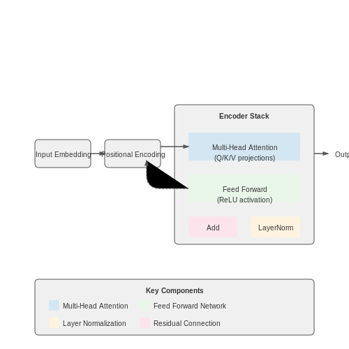
The Transformer model, introduced by Vaswani et al. in 2017, revolutionized natural language processing by replacing recurrent and convolutional layers with a purely attention-based mechanism. Its architecture consists of an encoder-decoder structure, where both components are composed of multiple identical layers with residual connections and layer normalization.
Encoder Structure
The encoder processes the input sequence through a stack of N identical layers (typically N = 6). Each layer contains two sub-layers:
- Multi-head self-attention mechanism - Computes attention weights between all positions in the input sequence.
- Position-wise feed-forward network - Applies the same fully connected network to each position separately.
Each sub-layer employs residual connections followed by layer normalization:
Decoder Structure
The decoder similarly consists of N identical layers, but with three sub-layers:
- Masked multi-head self-attention - Prevents positions from attending to subsequent positions.
- Multi-head encoder-decoder attention - Allows each position in the decoder to attend to all positions in the encoder output.
- Position-wise feed-forward network - Identical to the encoder's feed-forward sub-layer.
Attention Mechanism
The scaled dot-product attention computes alignment scores between queries (Q), keys (K), and values (V):
where dk is the dimension of the key vectors. Multi-head attention projects the queries, keys, and values h times with different learned linear projections, allowing the model to jointly attend to information from different representation subspaces:
Positional Encoding
Since the Transformer lacks recurrence or convolution, positional encodings are added to the input embeddings to inject information about the relative or absolute position of tokens in the sequence. The positional encodings use sine and cosine functions of different frequencies:
where pos is the position and i is the dimension. This choice allows the model to easily learn to attend by relative positions, since for any fixed offset k, PEpos+k can be represented as a linear function of PEpos.
Feed-Forward Networks
Each layer contains a fully connected feed-forward network applied to each position identically. This consists of two linear transformations with a ReLU activation in between:
The dimensionality of the inner layer (dff) is typically larger than the model dimension (dmodel), often dff = 2048 while dmodel = 512.
Layer Normalization and Residual Connections
Each sub-layer's output is normalized and combined with its input via residual connections:
This architecture choice helps mitigate the vanishing gradient problem in deep networks and enables more stable training. Layer normalization normalizes the activations across the feature dimension rather than the batch dimension, making it particularly effective for sequence processing tasks with variable lengths.
Positional Encoding and Tokenization
Tokenization in Transformer Models
Tokenization is the process of breaking down input text into smaller units called tokens, which serve as the atomic elements for neural processing. In transformer-based models like BERT and GPT, subword tokenization methods such as Byte Pair Encoding (BPE) and WordPiece are dominant. These algorithms balance vocabulary size and sequence length by splitting rare words into subword units while keeping frequent words intact. For example, "unhappiness" might be tokenized into ["un", "happiness"], allowing the model to handle out-of-vocabulary words through compositional meaning.
The mathematical formulation of tokenization involves optimizing a vocabulary V of size N to maximize the likelihood of the training corpus:
where M is the number of training examples, and P(x_i|V) is the probability of tokenizing sentence x_i given vocabulary V.
Positional Encoding Architecture
Since transformers lack recurrent or convolutional structures, they require explicit positional information to understand token order. Positional encoding injects this information using sinusoidal functions of varying frequencies:
where pos is the token position, i is the dimension index, and dmodel is the embedding dimension. This formulation allows the model to attend to relative positions through linear transformations, as proven by the trigonometric identity:
Implementation Considerations
Modern implementations often use learned positional embeddings instead of fixed sinusoidal patterns, particularly in models like BERT. The choice between fixed and learned embeddings involves trade-offs:
- Fixed sinusoidal encodings generalize better to longer sequences than seen during training
- Learned embeddings may capture task-specific positional patterns but require more data
For languages with complex morphology, hybrid tokenization strategies combining BPE with character-level CNNs have shown success. The tokenizer must preserve meaningful semantic units while avoiding excessive sequence length that would quadratically increase transformer attention costs.
Numerical Stability in Encoding
When combining token embeddings E and positional encodings PE, scaling factors must be carefully chosen to maintain stable gradients. The standard approach uses:
This scaling ensures the magnitude of embedding vectors remains approximately constant across different dimensions, preventing vanishing or exploding gradients in deep transformer stacks.

2. Data Preparation and Parallel Corpora
2.1 Data Preparation and Parallel Corpora
Parallel corpora form the backbone of supervised machine translation systems, providing aligned sentence pairs in source and target languages. The quality, size, and domain relevance of these corpora directly impact model performance. For transformer-based architectures, which rely heavily on large-scale data, preprocessing steps must preserve linguistic structure while optimizing computational efficiency.
Corpus Acquisition and Alignment
Publicly available parallel datasets include:
- Europarl: Proceedings of the European Parliament in 21 languages, offering domain-specific parliamentary discourse.
- UN Parallel Corpus: Multilingual translations of United Nations documents, characterized by formal diplomatic language.
- OpenSubtitles: Aligned movie subtitles exhibiting conversational and colloquial language patterns.
Sentence alignment algorithms typically employ statistical methods like:
where aj and bi represent sentences in the source and target languages respectively. Advanced alignment techniques incorporate:
- Dynamic programming for optimal pathfinding in alignment matrices
- Neural bilingual sentence embeddings for semantic matching
- Cross-lingual lexical similarity measures
Text Normalization and Tokenization
Transformer models require consistent tokenization schemes across languages. Subword tokenization methods address morphological diversity:
where x and y represent symbol pairs merged iteratively to build a vocabulary. For languages with complex scripts:
- Unicode normalization (NFKC) handles diacritics and composite characters
- SentencePiece enables language-agnostic tokenization
- Morphological analyzers decompose agglutinative languages (e.g., Turkish, Finnish)
Data Filtering and Cleaning
Quality thresholds should eliminate:
- Sentence pairs with length ratios exceeding 1.5:1
- Utterances with character repetition (>3 consecutive identical characters)
- Improper encoding or non-printable Unicode characters
Automatic filtering pipelines often employ:
where coefficients are tuned per language pair. For low-resource languages, backtranslation augments parallel data:
Train-Validation-Test Splits
Stratified sampling preserves:
- Domain distribution (e.g., legal, technical, conversational)
- Temporal coherence for time-sensitive data
- Lexical coverage across splits
For multilingual models, concatenated corpora require balanced representation:
where wi is the sampling weight for language i, L is the language set, and Ni is the corpus size for language i.
2.2 Loss Functions and Optimization Techniques
Cross-Entropy Loss for Sequence Prediction
Transformer models for language translation optimize the probability distribution over target vocabulary tokens given the source sequence. The standard loss function is the cross-entropy loss between the predicted token distribution pθ(yt|y<t, x) and the true token yt:
where T is the target sequence length. This formulation assumes teacher forcing during training, where the model receives the ground truth prefix y<t at each step. For large vocabularies, hierarchical softmax or sampled softmax techniques may be employed to reduce computational cost.
Label Smoothing
Standard cross-entropy encourages overconfidence in predictions. Label smoothing addresses this by redistribhing probability mass from the ground truth token to other tokens:
where ε is the smoothing parameter (typically 0.1) and K is the vocabulary size. This regularization technique improves model calibration and generalization, particularly for low-resource language pairs.
Optimization Strategies
Adam with Warmup
Transformers typically use Adam optimization with learning rate warmup. The learning rate schedule combines linear warmup for the first n steps followed by inverse square root decay:
where n is typically 4,000-40,000 steps. This prevents early instability from high variance gradients while allowing rapid convergence later in training.
Gradient Clipping
To mitigate exploding gradients in deep architectures, global gradient clipping scales gradients when their norm exceeds threshold τ:
Typical values for τ range from 0.1 to 10.0. This is particularly critical in transformer models due to the depth of the decoder stack and residual connections.
Advanced Techniques
Recent work has introduced several improvements to the standard optimization pipeline:
- Mixed Precision Training: Using FP16 for activations and FP32 for master weights reduces memory usage while maintaining stability via loss scaling.
- Gradient Accumulation: Enables effective batch sizes larger than GPU memory limits by accumulating gradients over multiple forward-backward passes.
- Learning Rate Scheduling: Cosine annealing with restarts has shown promise for transformer fine-tuning, particularly in multilingual settings.
The choice of optimization parameters significantly impacts model convergence and final performance, with optimal settings often varying across language pairs and dataset sizes. Empirical studies suggest transformer models are particularly sensitive to the warmup period and peak learning rate.
2.3 Handling Low-Resource Languages
Transformer models excel in high-resource language pairs but face significant challenges with low-resource languages due to limited parallel corpora. The scarcity of training data leads to poor generalization, lexical sparsity, and suboptimal embeddings. Addressing these issues requires specialized techniques that go beyond standard transfer learning.
Data Augmentation Strategies
Back-translation is a widely adopted method for synthetic data generation. Given a monolingual corpus in the low-resource target language L, sentences are translated to a high-resource language H using a pretrained model, then back-translated to L. The process can be formalized as:
Noise injection techniques further diversify the synthetic data. These include:
- Token dropout: Randomly masking tokens with probability p to improve robustness
- Word shuffling: Permuting words within a local window to simulate flexible word order
- Synonym replacement: Swapping words with semantically similar alternatives from a lexicon
Cross-Lingual Transfer Learning
Multilingual pretraining frameworks like mBERT and XLM-R leverage shared subword representations across languages. The key insight is that languages with overlapping subword tokens in the vocabulary space can transfer knowledge more effectively. For a vocabulary V shared across N languages, the embedding matrix E ∈ ℝ|V|×d learns cross-lingual patterns through:
where D combines monolingual corpora from multiple languages. Language-adversarial training can further improve cross-lingual transfer by minimizing the discriminator's ability to predict the language of hidden states:
Architectural Adaptations
For extremely low-resource scenarios (< 100k parallel sentences), modifying the transformer architecture itself becomes necessary. Two effective approaches include:
- Shared encoder-decoder frameworks: The encoder processes both source and target languages, while language-specific adapters (small feed-forward networks inserted between layers) customize outputs
- Dynamic vocabulary expansion: Gradually adding new subword tokens during fine-tuning based on frequency analysis of the target language
Recent work on mixture-of-experts architectures shows promise, where different model components activate based on the input language. The gating function G(x) routes examples to specialized experts:
Evaluation Challenges
Standard BLEU scores often fail to capture translation quality for low-resource languages due to:
- Lack of reference translations for many test sets
- Mismatches between the domains of available test sets and real-world usage
- Over-reliance on surface-level n-gram matching that ignores morphological richness
Alternative metrics like COMET (Crosslingual Optimized Metric for Evaluation of Translation), which uses pretrained multilingual encoders to assess semantic similarity, have shown better correlation with human judgments for low-resource pairs.
3. Transfer Learning with Pretrained Models
3.1 Transfer Learning with Pretrained Models
Mechanisms of Transfer Learning in Transformers
Transformer-based models leverage transfer learning through pretraining on large corpora followed by fine-tuning on domain-specific data. The pretraining phase learns universal linguistic patterns via self-supervised objectives like masked language modeling (MLM) or next sentence prediction (NSP). The key mathematical operation enabling this is the multi-head attention mechanism:
where Q, K, and V represent queries, keys, and values respectively, and dk is the dimension of the key vectors. During fine-tuning, only the final task-specific layers are modified while the pretrained attention mechanisms remain intact.
Parameter-Efficient Fine-Tuning Strategies
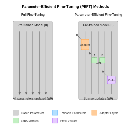
For large models like mT5 or BLOOM, full fine-tuning becomes computationally prohibitive. Recent approaches focus on modifying only a small subset of parameters:
- Adapter Layers: Insert small bottleneck feed-forward networks between transformer layers
- LoRA (Low-Rank Adaptation): Decomposes weight updates into low-rank matrices: ΔW = BA where B ∈ ℝd×r, A ∈ ℝr×k with r ≪ min(d,k)
- Prefix Tuning: Prepends trainable continuous vectors to the input sequence
Cross-Lingual Transfer Learning
Multilingual models like XLM-R demonstrate zero-shot transfer capabilities through shared subword vocabularies and aligned embedding spaces. The alignment is achieved by:
where ei and ej are embeddings of translation pairs, and M is a learned linear transformation. This enables knowledge transfer from high-resource to low-resource languages.
Practical Implementation Considerations
When fine-tuning pretrained transformers for translation tasks:
from transformers import AutoModelForSeq2SeqLM, Seq2SeqTrainingArguments

model = AutoModelForSeq2SeqLM.from_pretrained("google/mt5-base")
training_args = Seq2SeqTrainingArguments(
    output_dir="./results",
    per_device_train_batch_size=8,
    gradient_accumulation_steps=4,
    learning_rate=3e-5,
    num_train_epochs=3,
    fp16=True,
    save_total_limit=2
)
Critical hyperparameters include the learning rate (typically 1e-5 to 5e-5), batch size (adjusted via gradient accumulation), and dropout rate (0.1-0.3 for regularization). Mixed precision training (fp16) is essential for large models.
Domain Adaptation Techniques
For specialized domains (medical, legal), continued pretraining on in-domain corpora before task-specific fine-tuning yields significant improvements. The domain-adaptive pretraining objective combines:
where TLM denotes translation language modeling, jointly predicting masked tokens in parallel sentences. The mixing coefficient λ typically starts at 0.5 and anneals to 0.3.

Metrics for Translation Quality (BLEU, METEOR)
BLEU (Bilingual Evaluation Understudy)
The BLEU score, introduced by Papineni et al. in 2002, is a precision-based metric that compares a machine-generated translation against one or more human reference translations. It operates by computing n-gram overlaps between the candidate and reference texts, with a brevity penalty to penalize overly short outputs.
The core components of BLEU are:
- Modified n-gram precision: For each n-gram in the candidate translation, count how many times it appears in any reference translation, then divide by the total number of n-grams in the candidate.
- Brevity penalty (BP): Applied to prevent artificially high scores for very short translations.
Where:
- $$p_n$$ is the modified precision for n-grams of length $$n$$
- $$w_n$$ are weights (typically uniform: $$w_n = 1/N$$)
- $$BP = \min\left(1, e^{1 - \frac{r}{c}}\right)$$, with $$r$$ being the effective reference length and $$c$$ the candidate length
In practice, BLEU is typically computed for n-grams up to length 4 (BLEU-4). While widely adopted due to its simplicity and correlation with human judgment at the corpus level, BLEU has limitations in handling synonyms, paraphrasing, and grammatical correctness.
METEOR (Metric for Evaluation of Translation with Explicit ORdering)
Developed by Banerjee and Lavie in 2005, METEOR addresses several BLEU limitations by incorporating:
- Explicit word-matching with synonym support via WordNet
- A harmonic mean of precision and recall (rather than just precision)
- Penalties for poor word order alignment
The METEOR score is computed as:
Where:
- $$F_{\text{mean}}$$ is the harmonic mean of precision ($$P$$) and recall ($$R$$): $$\frac{10PR}{R + 9P}$$
- $$\text{Penalty}$$ accounts for fragmentation of matches
- $$\gamma$$ and $$\theta$$ are tunable parameters (default 0.5 and 3 respectively)
The fragmentation penalty is calculated based on the number of "chunks" (contiguous matching word sequences) in the alignment:
Comparative Analysis
While both metrics range from 0 to 1 (with 1 indicating perfect translation), they exhibit different behaviors:
- Granularity: BLEU operates at corpus level while METEOR can score individual sentences more reliably
- Recall sensitivity: METEOR's incorporation of recall makes it more sensitive to information omission
- Linguistic knowledge: METEOR's use of WordNet enables better handling of synonyms and paraphrasing
- Word order: METEOR explicitly penalizes disordered translations through its fragmentation penalty
Empirical studies show METEOR correlates better with human judgments at the sentence level (0.964 vs BLEU's 0.817 Pearson correlation in the original paper), though both remain imperfect proxies for translation quality. Modern systems often report both metrics alongside human evaluations.
Practical Implementation Considerations
When implementing these metrics:
- For BLEU, the standard implementation uses case-insensitive tokenization (typically with 13a tokenizer from mteval-v13a.pl)
- METEOR requires WordNet installation and proper lemma/stemming configuration
- Both metrics benefit from multiple reference translations (4+ references show diminishing returns)
- Confidence intervals should be reported when comparing systems (e.g., via bootstrap resampling)
3.3 Common Pitfalls and Overfitting
Overfitting in Transformer-Based Translation
Transformer models, despite their state-of-the-art performance, are particularly susceptible to overfitting due to their massive parameter counts and self-attention mechanisms. The key symptom manifests as excellent performance on training data but poor generalization to unseen validation or test sets. For a model with parameters θ, training loss Ltrain(θ) decreases while validation loss Lval(θ) increases after a certain point:
Primary Causes
- Excessive model capacity: Modern transformers (e.g., BERT, GPT) often have hundreds of millions of parameters, enabling them to memorize training samples rather than learn generalizable patterns.
- Data scarcity: High-quality parallel corpora for low-resource language pairs are limited, exacerbating overfitting risks.
- Attention mechanism vulnerabilities: Self-attention heads may develop spurious correlations that don't generalize.
Diagnostic Techniques
Effective detection requires monitoring multiple metrics beyond just loss:
Additionally, track:
- Perplexity divergence between training and validation sets
- Attention head diversity scores
- Gradient norm distributions during training
Mitigation Strategies
Regularization Methods
Effective regularization for transformers requires careful balancing:
Where λ1 controls L2 weight decay and λ2 modulates dropout rates across layers. Empirical studies show:
- Attention dropout rates between 0.1-0.3 work best for most translation tasks
- Layer-wise adaptive weight decay outperforms global L2 regularization
Data-Centric Approaches
Effective data augmentation techniques for translation include:
- Back-translation: Generate synthetic training pairs via reverse translation
- Subword regularization: Vary tokenization during training to improve robustness
- Dynamic masking: Randomly mask portions of input sequences
Architectural Solutions
Recent advances propose structural modifications to inherently reduce overfitting:
- Reversible transformers: Reduce memory footprint enabling larger effective batch sizes
- Mixture-of-experts: Sparse activation patterns prevent co-adaptation
- Cross-layer parameter sharing: Decreases total parameter count while maintaining capacity
Practical Implementation Considerations
When implementing these techniques in frameworks like PyTorch or TensorFlow:
# Example of implementing label smoothing in PyTorch
class LabelSmoothingLoss(nn.Module):
    def __init__(self, classes, smoothing=0.1):
        super().__init__()
        self.confidence = 1.0 - smoothing
        self.smoothing = smoothing
        self.classes = classes

    def forward(self, pred, target):
        pred = pred.log_softmax(dim=-1)
        true_dist = torch.zeros_like(pred)
        true_dist.fill_(self.smoothing / (self.classes - 1))
        true_dist.scatter_(1, target.unsqueeze(1), self.confidence)
        return torch.mean(torch.sum(-true_dist * pred, dim=-1))
Key hyperparameters to monitor include:
- Early stopping patience intervals
- Learning rate warmup steps
- Gradient clipping thresholds

4. Multilingual and Zero-Shot Translation
Multilingual and Zero-Shot Translation
Transformer-based models have revolutionized multilingual translation by enabling a single model to handle multiple language pairs without task-specific architectures. The key innovation lies in the model's ability to generalize across languages by leveraging shared representations in the embedding space. This is achieved through a combination of techniques, including language-specific embeddings, cross-lingual attention mechanisms, and large-scale multilingual pretraining.
Multilingual Training Paradigm
Multilingual models are trained on parallel corpora spanning multiple language pairs. The training objective remains the same as standard sequence-to-sequence learning, but the model learns to condition its outputs on both the input text and a target language token. The loss function for a multilingual model with N languages can be expressed as:
where Dij represents parallel data between languages i and j, x is the source sentence, y is the target sentence, and lj is the target language identifier.
Zero-Shot Translation Mechanism
Zero-shot translation emerges as a byproduct of multilingual training, where the model learns to translate between language pairs never explicitly seen during training. This capability stems from the model's development of an interlingua representation - a language-agnostic semantic space where sentences with equivalent meanings across languages map to similar vectors. The attention mechanism plays a crucial role in this process:
where queries (Q), keys (K), and values (V) are learned representations that become language-agnostic through multilingual training.
Practical Implementation Challenges
Several practical considerations affect multilingual translation performance:
- Language Imbalance: High-resource languages may dominate model capacity at the expense of low-resource ones.
- Vocabulary Design: Shared subword vocabularies must balance language coverage with token efficiency.
- Directional Bias: Some translation directions may perform better than others due to training data distribution.
Modern approaches address these challenges through techniques like temperature-based sampling during training and vocabulary balancing algorithms. For instance, the temperature-scaled sampling probability for language pair (i,j) is computed as:
where α is typically set between 0.2 and 0.5 to upweight low-resource language pairs.
Architectural Enhancements
State-of-the-art multilingual transformers incorporate several architectural modifications:
- Language-Specific Components: Some implementations use separate attention heads or feed-forward layers for different language families.
- Adaptive Softmax: Efficient output layers that handle large vocabularies across multiple languages.
- Language-Agnostic Middle Layers: Intermediate layers designed to promote language-independent representations.
These enhancements are particularly evident in models like mBART and NLLB, which demonstrate strong zero-shot capabilities across hundreds of languages while maintaining parameter efficiency through careful architectural design.

4.2 Model Compression and Efficiency
Quantization
Transformer models, particularly large-scale variants like BERT and GPT, require significant computational resources due to their high-precision floating-point parameters. Quantization reduces memory footprint and accelerates inference by converting 32-bit floating-point weights (FP32) to lower-bit representations (e.g., INT8 or FP16). The process involves mapping full-precision values to a discrete set:
where Δ is the quantization step size and Z is the zero-point offset. Post-training quantization (PTQ) applies this transformation after training, while quantization-aware training (QAT) simulates quantization effects during training to minimize accuracy loss.
Pruning
Pruning removes redundant weights or attention heads without significantly degrading model performance. Structured pruning eliminates entire neurons or layers, while unstructured pruning targets individual weights. A common approach is magnitude-based pruning, where weights below a threshold τ are zeroed out:
Iterative pruning, combined with fine-tuning, often yields better results than one-shot pruning. Recent work also explores lottery ticket hypotheses, identifying sparse subnetworks that retain performance when trained in isolation.
Knowledge Distillation
Knowledge distillation (KD) transfers knowledge from a large teacher model to a smaller student model. The student is trained not only on ground-truth labels but also on softened teacher outputs via a temperature-scaled softmax:
where T controls the smoothness of the distribution. The student’s loss function combines task-specific loss (Ltask) and distillation loss (LKD):
Variants like miniLM and DistilBERT demonstrate that students can achieve 90%+ of teacher performance with 50% fewer parameters.
Efficient Attention Mechanisms
The standard self-attention mechanism in transformers has O(n²) complexity, making it impractical for long sequences. Sparse attention patterns, such as:
- Local attention (restricting attention to a fixed window around each token),
- Strided attention (attending to every k-th token),
- Block-sparse attention (grouping tokens into fixed-size blocks)
reduce complexity to O(n√n) or O(n log n). The Longformer and BigBird models leverage these patterns for efficient processing of documents with thousands of tokens.
Hardware-Aware Optimization
Deploying compressed models requires co-design with hardware accelerators. Techniques include:
- Operator fusion: Combining consecutive operations (e.g., layer normalization and residual addition) to reduce memory bandwidth.
- Kernel optimization: Tailoring matrix multiplications for GPU tensor cores or TPU systolic arrays.
- Dynamic execution: Skipping layers or heads conditionally via early-exit strategies or adaptive computation time (ACT).
Tools like TensorRT and ONNX Runtime automate hardware-specific optimizations for quantized and pruned models.

4.3 Adversarial Attacks and Robustness
Transformer-based language models, despite their state-of-the-art performance in translation tasks, are vulnerable to adversarial attacks—carefully crafted perturbations to input text that induce incorrect translations. These attacks exploit the model's sensitivity to small, often imperceptible changes in the input space. Adversarial examples can be generated via gradient-based optimization or heuristic search methods, targeting the model's attention mechanisms or embedding layers.
Types of Adversarial Attacks
Adversarial attacks on translation models broadly fall into three categories:
- Token-level perturbations: Subtle modifications to individual tokens, such as synonym substitution or character-level edits (e.g., "cat" → "caṭ"), which preserve semantic meaning but alter model predictions.
- Gradient-based attacks: Leveraging the model's differentiable structure to compute input gradients, such as Fast Gradient Sign Method (FGSM) or Projected Gradient Descent (PGD), to maximize translation error.
- Attention manipulation: Forcing the model to attend to incorrect input segments by injecting distracting tokens or reordering source sentences.
Mathematical Formulation
Given a translation model f and input sequence x, an adversarial example x' is crafted to maximize a loss function L while constrained by a perturbation budget ε:
where ||·||p is the Lp-norm (typically L2 or L∞), and y is the ground-truth translation. For gradient-based attacks, the perturbation is often computed as:
Defensive Strategies
Improving robustness against adversarial attacks involves both training-time and inference-time techniques:
- Adversarial training: Augmenting the training data with adversarial examples to improve model resilience, formulated as a min-max optimization problem:
- Randomized smoothing: Applying random noise or dropout during inference to obscure adversarial perturbations.
- Input sanitization: Detecting and filtering adversarial tokens via outlier detection in embedding space or vocabulary constraints.
Case Study: Attacking and Defending Transformer Translation
Recent studies demonstrate that even state-of-the-art models like mBART or T5 suffer significant performance drops under adversarial conditions. For instance, injecting just 5% adversarial tokens can reduce BLEU scores by over 30%. Defenses such as adversarial fine-tuning or gradient masking have shown promise, but trade-offs between robustness and standard accuracy remain an open challenge.
5. Bias in Training Data and Outputs
5.1 Bias in Training Data and Outputs
Transformer-based language translation models inherit biases present in their training data, which propagate into translated outputs. These biases manifest as skewed representations of gender, race, culture, and socio-political contexts. For instance, a model trained on predominantly male-authored texts may default to masculine pronouns when translating gender-neutral source sentences. The bias amplification arises from the model's objective function, which maximizes the likelihood of observed training data without explicit fairness constraints.
Mathematical Formulation of Bias Propagation
The translation probability distribution P(y|x) learned by a transformer model reflects the empirical distribution of the training corpus. Given a source sentence x and target sentence y, the model's output bias can be quantified through the divergence between the model's predictions and an ideal unbiased distribution Q(y|x):
where DKL represents the Kullback-Leibler divergence, and Q(y|x) is constructed to enforce demographic parity or other fairness criteria. The bias magnitude increases with the divergence value.
Common Bias Types in Translation Models
- Gender bias: Models associate certain professions with specific genders (e.g., "nurse" → feminine, "engineer" → masculine) due to imbalanced training examples.
- Cultural bias: Default translations favor Western perspectives when converting culturally specific concepts (e.g., translating "tea" as "black tea" for Chinese inputs).
- Lexical bias: Words with multiple meanings receive skewed translations based on frequency (e.g., "bank" translated as financial institution more often than riverbank).
Measuring Translation Bias
The Bias Score for a translation model can be computed using counterfactual evaluation. For a set of gender-neutral source sentences {xi}, we measure the probability difference between masculine and feminine translations:
where yim and yif are masculine and feminine variants of the same translation. Scores closer to 1 indicate stronger bias.
Debiasing Techniques
Data-Augmentation Methods
Generating balanced training data through:
- Counterfactual data augmentation (CDA): Creating gender-swapped versions of existing sentences
- Adversarial filtering: Removing samples that contribute disproportionately to biased predictions
Architectural Modifications
- Bias-controlled attention heads: Adding fairness constraints to specific attention mechanisms
- Debiased embedding spaces: Post-processing word embeddings to remove directional bias components
Training Objectives
Augmenting the standard cross-entropy loss LCE with fairness terms:
where λ controls the strength of debiasing. Recent work also employs contrastive learning to pull biased and unbiased representations closer in the latent space.
Case Study: Gender Bias in Google Translate
A 2020 analysis revealed Google Translate produced masculine translations for 67% of gender-neutral Turkish sentences (a pro-drop language). After implementing counterfactual data augmentation, the bias dropped to 53%, demonstrating that technical interventions can mitigate but not eliminate bias without addressing root causes in data collection.
5.2 Fairness in Language Representation
Transformer-based language models, despite their remarkable performance, often exhibit biases in translation due to imbalances in training data. These biases manifest as skewed representations of gender, race, and cultural context, particularly for low-resource languages. The root cause lies in the disproportionate distribution of data across languages and dialects, leading to systemic underrepresentation.
Quantifying Bias in Embedding Spaces
Bias in translation models can be formalized through geometric properties of word embeddings. Let wi represent the embedding vector for a word in language L1, and wj its translation in L2. The alignment error E captures directional bias:
where A is the linear transformation matrix between language pairs. When certain demographic groups exhibit consistently higher E values, this indicates systemic bias in the representation space.
Debiasing Techniques
Three principal methods exist for mitigating bias in multilingual transformers:
- Adversarial Debiasing: Introduces a discriminator network that penalizes the model for encoding protected attributes (gender, race) in the latent space.
- Counterfactual Data Augmentation: Generates synthetic parallel corpora with swapped demographic attributes to balance representation.
- Geometric Constraint Optimization: Directly modifies the loss function to enforce equal distances between neutral and biased terms in the embedding space.
The geometric approach modifies the standard cross-entropy loss LCE with a fairness regularizer:
where μg represents the mean embedding vector for demographic group g, and λ controls the regularization strength.
Case Study: Gender Bias in English-Spanish Translation
Recent evaluations of Transformer models (e.g., mBERT, XLM-R) reveal that occupational terms exhibit strong gender skews. For instance, "nurse" translates to "enfermera" (feminine) 87% of the time, while "engineer" becomes "ingeniero" (masculine) 92% of the time, despite gender-neutral source terms. This occurs because:
- Training data overrepresents historical gender stereotypes
- Attention mechanisms amplify frequent co-occurrence patterns
- Subword tokenization fragments gender markers in morphologically rich languages
Mitigation requires both data-level interventions (rebalancing corpora) and architectural modifications (gender-aware attention heads).
Evaluating Fairness Metrics
Standard evaluation protocols must extend beyond BLEU scores to include:
where S is a set of stereotype test cases, and 𝕀 is the indicator function. The StereoSet benchmark provides language-specific tests for 17 languages, measuring both stereotype recognition and generation.
Current state-of-the-art models still show significant gaps: XLM-R exhibits 23% higher bias scores for African American Vernacular English (AAVE) compared to Standard American English in translation tasks, highlighting the need for dialect-aware training strategies.

5.3 Mitigation Strategies
Transformer-based translation models, despite their effectiveness, exhibit several failure modes including hallucination, gender bias, and domain mismatch. Advanced mitigation strategies address these through architectural modifications, training paradigms, and post-processing techniques.
Handling Rare Words via Subword Tokenization
The Byte Pair Encoding (BPE) algorithm decomposes rare words into subword units, balancing vocabulary size and out-of-vocabulary robustness. Given a corpus with word frequencies, BPE iteratively merges the most frequent symbol pairs:
where V is the current vocabulary. This produces hybrid representations like "unfortunate" → ["un", "##fort", "##unate"], enabling compositionality for low-frequency terms.
Attention Head Diversity Regularization
To prevent attention heads from collapsing to redundant patterns, the diversity loss term penalizes similarity between attention matrices Ai and Aj:
Empirical studies show this increases the model's capacity to capture distinct linguistic phenomena (syntax vs. semantics) across heads.
Counterfactual Data Augmentation
For gender bias mitigation, training batches are augmented with counterfactual examples where gendered pronouns are systematically swapped. The loss function incorporates a consistency term:
where xm→f denotes male-to-female pronoun substitution. This forces invariant representations across gender contexts.
Dynamic Temperature Scaling
To address overconfidence in low-probability predictions, the softmax temperature τ is dynamically adjusted based on sequence entropy:
The learned parameters W allow per-head adaptation, sharpening or smoothing distributions based on contextual uncertainty.
Gradient Accumulation for Long Sequences
When processing documents exceeding the model's maximum sequence length, gradient accumulation enables effective batch processing:
for i, (segments, labels) in enumerate(long_document_loader):
    # Forward pass on segment batch
    outputs = model(segments)
    loss = criterion(outputs, labels) / accumulation_steps

    # Backward pass with scaled loss
    loss.backward()

    # Update weights only after accumulating N batches
    if (i + 1) % accumulation_steps == 0:
        optimizer.step()
        optimizer.zero_grad()
This maintains stable training while handling arbitrarily long inputs through memory-efficient segmentation.
6. Key Research Papers
6.1 Key Research Papers
- PDF Text2Gloss: Translation into Sign Language Gloss with Transformers — Abstract Translation of text into its corresponding sign language gloss annotations is a key step in end-to-end sign language translation, as well as useful for sign language interpreters. We apply a transformer model to the text to gloss task, providing a baseline for further applications of transformers on this task.
- Learning Deep Transformer Models for Machine Translation — Transformer is the state-of-the-art model in recent machine translation evaluations. Two strands of research are promising to im-prove models of this kind: the first uses wide networks (a.k.a. Transformer-Big) and has been the de facto standard for the de-velopment of the Transformer system, and the other uses deeper language representation but ...
- Introduction to Transformers: an NLP Perspective - arXiv.org — Abstract Transformers have dominated empirical machine learning models of natural language pro-cessing. In this paper, we introduce basic concepts of Transformers and present key tech-niques that form the recent advances of these models. This includes a description of the standard Transformer architecture, a series of model refinements, and common applica-tions. Given that Transformers and ...
- Machine Translation with Transformers - uni-stuttgart.de — The Transformer translation model (Vaswani et al., 2017), which relies on self-attention mechanisms, has achieved state-of-the-art performance in recent neural machine translation (NMT) tasks.
- A comprehensive survey on applications of transformers for deep ... — One paper aimed to categorize Transformer vision-language models based on tasks, providing summaries of their corresponding advantages and disadvantages. Furthermore, this survey covered video-language pre-trained models, classifying them into single-stream and multi-stream structures while comparing their performance (Ruan & Jin, 2022).
- PDF Promises and perils of using Transformer-based models for SE research — Fourth, we report on poor model generalization for the most popular benchmarks and datasets on Bug Fixing and Code Summarization tasks. We frame our contributions in terms of promises and perils, and document the numerous practical issues in advancing future research on transformer-based models for code-related tasks.
- Transformers and large language models in healthcare: A review — This paper aims to provide a comprehensive review of Transformer models utilized across multiple healthcare data modalities while focusing on notable architectural changes undergone by the original Transformer model through this process of evolution.
- "Enhancing and Exploring the Use of Transformer Models in NLP Tasks" — The advent of transformer models has revolutionized the field of Natural Language Processing (NLP), offering unprecedented capabilities in various tasks such as text generation, machine ...
- Transformer Architectures | SpringerLink — Transformer architectures have revolutionized the field of natural language processing (NLP) and have become the backbone of many state-of-the-art models. Unlike traditional RNNs and CNNs, transformers rely entirely on a mechanism known as self-attention to draw global dependencies between input and output.
- Machine Translation of English Language Using the ... - ResearchGate — The Transformer-based translation model mainly improves the performance at the cost of growing model sizes and complexity, usually requiring million-scale parameters.
6.2 Open-Source Implementations
- Transformers and large language models in healthcare: A review — Yang et al. developed an open-source Transformers package with four transformer-based models, BERT , ALBERT , RoBERTa , and ELECTRA , pretrained on MIMIC-III dataset for clinical concept extraction. Peng et al. [ 83 ] used transfer learning to fine-tune BERT [ 20 ] for concept extraction on BC5CDR [ 62 ] and ShARe/CLEF [ 110 ] datasets.
- Machine Translation with Transformers - uni-stuttgart.de — The Transformer translation model (Vaswani et al., 2017), which relies on self- ... input source language to its associated output target language in an end-to-end fashion (Wu et al., 2016). The architecture of NMT models often consists of an encoder and a decoder (Figure 1). Firstly, each word in the input sentence is fed separately into the
- Sign Language Translation with Transformers - Soutron Global — focuses on enhancing translation from sign language glosses to spoken language. The recent success of Transformers for NMT between spoken languages inspires us to adopt this architecture. We study Transformers for SLT in various setups, including techniques from spoken language processing that have not yet been applied to sign language.
- PDF Language Modeling with Deep Transformers — formance in language modeling using the Transformer decoder component [10-15]. The earliest example can be found in [10] where such models are investigated for text generation. Recent works on training larger and deeper models [12,14,15] have shown further potential of the Transformer in language model-ing.
- An Improved Transformer-Based Neural Machine Translation Strategy ... — 2.1. Transformer. The transformer architecture resolves NMT solely by relying on the attention algorithm [].It has been proved that the transformer-based models are superior to the models using RNNs and CNN [1-4, 8, 9].Like RNNs and CNN, the standard transformer-based model employs the encoder-to-decoder structure for NMT [].This structure maps the source sequence to a hidden state matrix as ...
- Learning Deep Transformer Models for Machine Translation - arXiv.org — Transformer is the state-of-the-art model in recent machine translation evaluations. Two strands of research are promising to im-prove models of this kind: the first uses wide networks (a.k.a. Transformer-Big) and has been the de facto standard for the de-velopment of the Transformer system, and the other uses deeper language representation
- Demystifying Transformers: A Comprehensive Roadmap to ... - Medium — 6.2 Integration with Applications - Integrate transformer models into real-world applications, such as chatbots, recommendation systems, or language translation services. 7.
- Learning Deep Transformer Models for Machine Translation — PDF | On Jan 1, 2019, Qiang Wang and others published Learning Deep Transformer Models for Machine Translation | Find, read and cite all the research you need on ResearchGate
- MarianCG: a code generation transformer model inspired by machine ... — Code generation is a significant field that can predict and generate suitable code as output from the natural language as the input source. The increasing of code generation tools with accuracy and optimization tools can help to increase the productivity of the programming tools [].Application Programming Interfaces or APIs make software development and innovation easier by allowing ...
- Transformer_translate.ipynb - Colab - Google Colab — In this notebook we will see how to use this library for a translation task by exploring the necessary steps. We will see how to define a problem, generate the data, train the model and test the quality of it, and we will translate our sequences and we visualize the attention. We will also see how to download a pre-trained model. [ ]
6.3 Recommended Books and Courses
- Introduction to Transformer Models for NLP: Using BERT, GPT, and More ... — Video description 10+ Hours of Video Instruction Learn how to apply state-of-the-art transformer-based models including BERT and GPT to solve modern NLP tasks. Overview Introduction to Transformer Models for NLP LiveLessons provides a comprehensive overview of transformers and the mechanisms—attention, embedding, and tokenization—that set the stage for state-of-the-art NLP models like BERT ...
- Transformer with TensorFlow - Armin Norouzi — It is mainly used for tasks such as language translation, text summarization, and language modelling. The Transformer model consists of an encoder and a decoder that work together to process input sequences and generate output sequences. The encoder processes the input sequence and produces a hidden representation of the input. ... 2.4.6.3. The ...
- Machine Translation with Transformers - uni-stuttgart.de — The Transformer translation model (Vaswani et al., 2017), which relies on self-attention mechanisms, has achieved state-of-the-art performance in recent neural ... as language model, translation model, and reordering model. The structure of the NMT models is simpler than phrase-based models. NMT aims at building and
- Book NLP with Transformers: Fundamentals and Core Applications by ... — The book also covers the evolution of transformer architecture from early models like the original Transformer to newer variants like BERT, GPT, and T5. Each model is explored in context, with examples demonstrating their specific strengths in tasks like text classification, machine translation, and more.
- PDF Assignment 3: Transformer Language Modeling Dataset and Code — Part 2: Transformer for Language Modeling (50 points) In this second part, you will implement a Transformer language model. This should build heavily off of what you did for Part 1, although for this part you are allowed to use off-the-shelf Transformer components. For this part, we use the first 100,000 characters oftext8 as the training set.
- Transformers for Machine Learning A Deep Dive - Routledge — Transformers are becoming a core part of many neural network architectures, employed in a wide range of applications such as NLP, Speech Recognition, Time Series, and Computer Vision. Transformers have gone through many adaptations and alterations, resulting in newer techniques and methods. Transformers for Machine Learning: A Deep Dive is the first comprehensive book on transformers. Key ...
- Building a Simple Language Translation Tool Using a Pre-Trained ... — English to Hindi Translator using Pre-trained Translation Model Step 1: Import Necessary Libraries. The first step involves importing the libraries required for translation and building the interactive interface. In this case, we need the transformers library for the translation model and gradio for creating a web interface.
- Learning Deep Transformer Models for Machine Translation — PDF | On Jan 1, 2019, Qiang Wang and others published Learning Deep Transformer Models for Machine Translation | Find, read and cite all the research you need on ResearchGate
- Sign Language Translation Using Multi Context Transformer — Usually, sign language translation models comprise of two networks: (i) A 2D convolution network like VGG to extract spatial features in a d-dimensional feature space from the video by processing individual frames; (ii) A sequence model like Long Short-Term Memory to map the extracted d-dimensional feature vectors to the output translation ...
- Transformers For Machine Learning A Deep Dive (Uday Kamath ... - Scribd — The best model for both approaches are chosen based on the best fit on the validation data. To understand how the attention mechanism operates during the translation process, we plot a few examples of the decoded attention out-puts highlighting where the decoder is attending as shown in Fig. 2.17. Transformers: Basics and Introduction 35