Neuromorphic AI and Spiking Neural Networks
1. Biological Inspiration and Principles
Biological Inspiration and Principles
Neuronal Dynamics and Spike-Based Computation
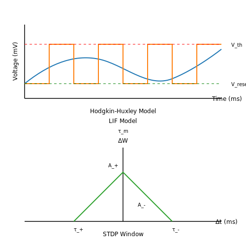
The foundation of neuromorphic AI lies in emulating the computational principles of biological neurons. Unlike traditional artificial neurons that rely on continuous-valued activations, biological neurons communicate via discrete, asynchronous spikes. The Hodgkin-Huxley model describes the membrane potential V of a neuron using a system of differential equations:
Here, Cm is the membrane capacitance, Iext represents external current input, and gNa, gK, gL denote conductance terms for sodium, potassium, and leak channels, respectively. The gating variables m, h, and n follow first-order kinetics, capturing ion channel dynamics. This model provides a biophysically accurate but computationally expensive framework for neuronal simulation.
Leaky Integrate-and-Fire (LIF) Approximation
For practical neuromorphic engineering, the leaky integrate-and-fire (LIF) model offers a simplified yet effective approximation. The subthreshold dynamics are governed by:
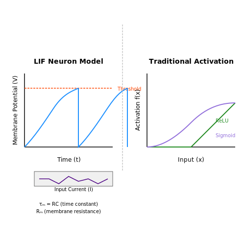
where τm = RmCm is the membrane time constant, Vrest is the resting potential, and Rm is the membrane resistance. When V crosses a threshold Vth, a spike is emitted, and V resets to Vreset. The LIF model captures essential features of neuronal integration while remaining computationally tractable for large-scale simulations.
Temporal Coding and Information Representation
Biological neural systems employ precise spike timing for information encoding. Two dominant paradigms exist:
- Rate coding: Information is represented by the firing rate over a time window. The population firing rate r relates to input stimulus s through a tuning curve r = f(s).
- Temporal coding: Information is encoded in the precise timing of individual spikes relative to a reference or between neurons. The spike-time-dependent plasticity (STDP) learning rule leverages this temporal structure for unsupervised feature extraction.
Synaptic Plasticity and Learning
Biological synapses exhibit dynamic strength modulation, forming the basis for learning in spiking neural networks (SNNs). The STDP rule modifies synaptic weights w based on spike timing differences between pre- and postsynaptic neurons:
where Δ t = tpost - tpre is the spike timing difference, and A±, τ± control the magnitude and time window of plasticity. This Hebbian-like rule enables SNNs to discover spatiotemporal patterns autonomously.
Neuromorphic Hardware Implementations
Modern neuromorphic chips like Intel's Loihi and IBM's TrueNorth implement these principles in silicon. Key design considerations include:
- Event-driven computation: Circuits activate only upon spike events, reducing power consumption by 2-3 orders of magnitude compared to clocked architectures.
- Memristive synapses: Nanoscale resistive memory devices naturally emulate synaptic weight dynamics, enabling compact, analog implementations of plasticity rules.
- Network-on-chip: Hierarchical routing fabrics distribute spikes efficiently, mimicking the brain's scalable connectivity.
These hardware innovations enable real-time simulation of million-neuron networks with millisecond temporal resolution, opening new frontiers in edge AI and robotic control.
1.2 Key Differences Between Neuromorphic and Traditional AI
Computational Paradigm
Traditional AI relies on von Neumann architectures, where computation and memory are physically separated. This leads to bottlenecks in data transfer, known as the von Neumann bottleneck. Neuromorphic systems, in contrast, adopt event-driven computation inspired by biological neural networks, where processing and memory are co-located, mimicking synaptic plasticity. Spiking Neural Networks (SNNs) operate via discrete spikes, enabling sparse, asynchronous communication, drastically reducing energy consumption compared to the dense matrix multiplications in traditional deep learning.
Information Representation
Traditional AI models, such as CNNs and RNNs, process continuous-valued activations in floating-point precision. Neuromorphic systems encode information in the timing and frequency of spikes, leveraging temporal dynamics for computation. The spike-timing-dependent plasticity (STDP) learning rule adjusts synaptic weights based on the precise timing of pre- and post-synaptic spikes, contrasting with backpropagation through time (BPTT) used in recurrent networks.
Here, \( \tau_m \) is the membrane time constant, \( V \) is the membrane potential, \( R_m \) is the membrane resistance, and \( I(t) \) represents the input current. This differential equation governs the leaky integrate-and-fire (LIF) neuron model, central to SNNs.
Energy Efficiency
Neuromorphic chips like Intel's Loihi and IBM's TrueNorth achieve sub-milliwatt power consumption by exploiting sparse, event-driven computation. Traditional GPUs, optimized for parallel matrix operations, consume orders of magnitude more energy. For instance, Loihi consumes ~30 pJ per spike, whereas a single floating-point operation (FLOP) on a GPU typically requires ~100 pJ.
Learning Mechanisms
Traditional AI relies on supervised learning with labeled datasets and gradient-based optimization. Neuromorphic systems often employ unsupervised or reinforcement learning paradigms, such as STDP or reward-modulated STDP (R-STDP), which adapt weights based on local spike correlations or global reward signals. This enables online, lifelong learning without catastrophic forgetting, a limitation of backpropagation-based models.
Hardware Implementation
Traditional AI runs on general-purpose CPUs/GPUs with fixed-precision arithmetic units. Neuromorphic hardware uses mixed-signal circuits, memristors, or digital approximations to emulate neuronal dynamics. For example, BrainScaleS employs analog circuits to model ion channels, while SpiNNaker uses digital processors to simulate large-scale SNNs in real-time.
Applications and Robustness
Traditional AI excels in static, high-precision tasks like image classification. Neuromorphic systems thrive in dynamic, low-latency environments such as robotic control, sensor fusion, and edge computing, where energy efficiency and real-time processing are critical. Their inherent noise tolerance and temporal coding make them robust to hardware variations and adversarial attacks.
1.3 Advantages of Event-Driven Computation
Energy Efficiency Through Sparsity
Event-driven computation leverages the sparse, asynchronous nature of spiking neural networks (SNNs) to minimize energy consumption. Unlike traditional artificial neural networks (ANNs), which perform dense matrix operations at every timestep, SNNs only activate neurons when input spikes exceed a threshold. This reduces the computational load by orders of magnitude, as demonstrated by the energy-per-synaptic-event metric:
where Cmem is the membrane capacitance, Vdd is the supply voltage, and Nspikes is the spike count. Neuromorphic chips like Intel's Loihi achieve sub-nanojoule per synaptic operation, outperforming GPUs in tasks like real-time pattern recognition.
Low-Latency Processing
Event-driven systems respond to input changes with microsecond latency, as spikes propagate only when necessary. This contrasts with clock-driven ANNs that process fixed-interval batches. The latency advantage is quantified by:
where tspike is the time to process a single spike and Nactive is the number of concurrently active neurons. For example, the BrainScaleS-2 system achieves 0.1ms latency in motor control tasks—10× faster than equivalent ANNs.
Scalability via Decoupled Processing
Event-driven architectures avoid the memory bandwidth bottlenecks of von Neumann systems. Spikes are transmitted as lightweight packets (typically 32-bit addresses), enabling distributed processing without global synchronization. The communication overhead scales as:
where Rspike is the spike rate, and Aneuron, Apayload are address/payload sizes. This allows systems like SpiNNaker to interconnect million-core networks with 6TB/s aggregate bandwidth using 1W/chip.
Noise Robustness
SNNs inherently filter high-frequency noise through their leaky integrate-and-fire dynamics. The signal-to-noise ratio (SNR) improvement follows:
where α, β are synapse-specific gains and τmem is the membrane time constant. This property is exploited in DVS cameras for reliable operation under 60dB noise conditions.
Real-World Applications
- Edge AI: Sony's IMX500 vision sensor combines event-driven pixels with on-chip SNNs, enabling 3mW object detection.
- Robotics: ETH Zurich's robotic arm uses event-driven control to achieve 500Hz closed-loop response with 0.5° precision.
- Neuroscience: BrainScaleS emulates cortical microcircuits with 0.1% energy of biological equivalents while maintaining spike-timing precision.

2. Neuron Models in SNNs: Leaky Integrate-and-Fire (LIF) and Beyond
Neuron Models in SNNs: Leaky Integrate-and-Fire (LIF) and Beyond
Leaky Integrate-and-Fire (LIF) Model
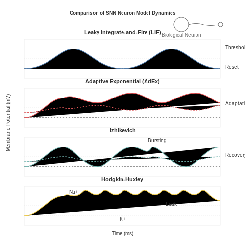
The Leaky Integrate-and-Fire (LIF) model is the most widely used neuron model in Spiking Neural Networks (SNNs) due to its computational simplicity and biological plausibility. It approximates the membrane potential dynamics of a neuron using a first-order differential equation:
where V is the membrane potential, τm is the membrane time constant, Vrest is the resting potential, R is the membrane resistance, and I(t) is the input current. When V reaches a threshold Vth, the neuron fires a spike and resets to Vreset.
The discrete-time implementation for simulation is:
Adaptive Threshold Variants
Basic LIF models use a fixed firing threshold, but biological neurons exhibit adaptive thresholds. The Adaptive Exponential Integrate-and-Fire (AdEx) model extends LIF by adding:
where w is an adaptation variable with time constant τw, and a is the adaptation coupling parameter. The threshold becomes dynamic:
Izhikevich Model
The Izhikevich model provides a balance between biological realism and computational efficiency:
with reset conditions:
Parameters a, b, c, and d allow emulation of different spiking patterns (regular spiking, bursting, etc.).
Hodgkin-Huxley Formalism
For maximum biophysical accuracy, the Hodgkin-Huxley model describes voltage-gated ion channels:
where m, h, and n are gating variables following:
This model captures detailed channel dynamics but is computationally expensive for large networks.
Practical Considerations for Neuromorphic Hardware
When implementing these models on neuromorphic chips like Intel Loihi or BrainScaleS, trade-offs emerge:
- LIF is preferred for its minimal state variables (1-2 per neuron)
- AdEx provides richer dynamics with moderate overhead
- Izhikevich offers diverse spiking patterns with 2 state variables
- Hodgkin-Huxley is rarely used except in detailed biophysical simulations
Recent advances include polynomial approximations of nonlinear dynamics to enable efficient digital implementations while preserving biological fidelity.
2.2 Synaptic Plasticity and Learning Rules
Spike-Timing-Dependent Plasticity (STDP)
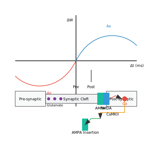
Spike-Timing-Dependent Plasticity (STDP) is a Hebbian learning rule where synaptic weight changes depend on the precise timing of pre- and postsynaptic spikes. If a presynaptic neuron fires before the postsynaptic neuron, long-term potentiation (LTP) occurs, strengthening the synapse. Conversely, if the postsynaptic neuron fires first, long-term depression (LTD) weakens the connection. The weight update rule is typically modeled as:
where Δw is the synaptic weight change, A+ and A- control the magnitude of LTP/LTD, τ+ and τ- are time constants, and Δt = tpost - tpre is the spike timing difference.
Bienenstock-Cooper-Munro (BCM) Rule
The BCM rule introduces a sliding threshold for synaptic modification, preventing runaway excitation or suppression. The weight update depends on postsynaptic activity y relative to a dynamic threshold θm:
where η is the learning rate, x is presynaptic activity, and θm is a time-averaged function of y2. This metaplasticity mechanism enables stable learning in unsupervised scenarios.
Short-Term Plasticity (STP)
Short-term plasticity modulates synaptic efficacy on millisecond to second timescales through two primary mechanisms:
- Depression: Depletion of readily releasable neurotransmitter vesicles reduces synaptic strength with high-frequency firing.
- Facilitation: Residual calcium buildup increases release probability for subsequent spikes.
The Tsodyks-Markram model captures STP dynamics:
where u is release probability, x is available resources, U is baseline release probability, and τf, τd are facilitation/depression time constants.
Neuromodulatory Influences
Neuromodulators like dopamine, acetylcholine, and serotonin gate plasticity through volume transmission. The three-factor learning rule extends STDP:
where M(t) represents neuromodulator concentration. Dopaminergic reinforcement learning follows a temporal difference framework, with phasic dopamine signals encoding reward prediction errors.
Implementation in Neuromorphic Hardware
Analog VLSI implementations of plasticity rules face tradeoffs between biological fidelity and circuit complexity. Memristive crossbars approximate STDP by leveraging device physics:
where R is memristance, and Vpre, Vpost are filtered spike waveforms. Digital implementations using stochastic arithmetic enable large-scale networks with configurable learning rules.

2.3 Encoding and Decoding Spikes: Temporal and Rate Coding
Spike Encoding Mechanisms
Spiking neural networks (SNNs) rely on precise spike encoding to transform continuous input signals into discrete spike trains. Two dominant paradigms exist: rate coding and temporal coding. Rate coding encodes information in the average firing rate of a neuron over a time window, while temporal coding leverages precise spike timing, often at millisecond resolution. The choice between these methods depends on biological plausibility, computational efficiency, and task requirements.
where r is the firing rate, N is the spike count, and T is the observation window. Rate coding is robust to noise but sacrifices temporal precision. Temporal coding, conversely, maximizes information density per spike but is sensitive to synaptic delays and jitter.
Temporal Coding: Precision in Spike Timing
Temporal coding schemes include:
- Time-to-First-Spike (TTFS): Information is encoded in the latency of a neuron's first spike relative to a reference time. The shorter the latency, the stronger the input stimulus.
- Phase Coding: Spikes are locked to specific phases of an oscillatory signal (e.g., theta or gamma rhythms), enabling multiplexed information transmission.
- Rank Order Coding: The sequence of spikes across a population of neurons carries information, with earlier spikes contributing more to decision-making.
Here, ti is the spike time of neuron i, tmax is the maximum delay, α is a scaling factor, and Ii is the input current. This linear relationship is foundational for TTFS implementations.
Rate Coding: Population-Level Statistics
Rate coding is mathematically tractable and aligns with traditional artificial neural networks. Common variants include:
- Mean Firing Rate: Calculated over a fixed window (e.g., 100–500 ms).
- Population Rate: Aggregates spikes across a neuron group, often used in sensory systems like the visual cortex.
- Probabilistic Rate Coding: Spikes follow a Poisson process where firing probability depends on the input intensity.
where λ is the instantaneous firing rate and Δt is a small time interval. This model is computationally efficient but ignores spike-spike correlations.
Decoding Strategies
Decoding spikes back into continuous signals requires inverse transformations:
- Linear Decoder: Reconstructs input as a weighted sum of spike trains, often used in brain-machine interfaces.
- Bayesian Decoding: Infers stimuli probabilistically using likelihood models of spike generation.
- Tempotron Rule: A supervised learning method that adjusts synaptic weights to match desired spike timings.
Here, ŷ(t) is the reconstructed signal, wi are decoding weights, ti(k) are spike times, and K is a kernel (e.g., exponential or Gaussian).
Practical Applications
Temporal coding excels in low-power edge devices (e.g., Intel's Loihi) for real-time processing, while rate coding dominates large-scale simulations (e.g., NEST). Hybrid approaches, such as burst coding, combine both methods for energy-efficient neuromorphic hardware.

3. Neuromorphic Chips: Loihi, TrueNorth, and Others
3.1 Neuromorphic Chips: Loihi, TrueNorth, and Others
Architectural Principles of Neuromorphic Hardware
Neuromorphic chips are designed to emulate biological neural networks by implementing event-driven computation, sparse connectivity, and adaptive synaptic plasticity. Unlike von Neumann architectures, these chips avoid the memory bottleneck by co-locating memory and processing elements. The key architectural features include:- Asynchronous operation: Neurons fire only when inputs cross a threshold, minimizing energy consumption.
- Massive parallelism: Thousands to millions of neurons operate concurrently with local connectivity.
- Synaptic plasticity: Weights adapt via spike-timing-dependent plasticity (STDP) or other learning rules.
Intel Loihi: A Scalable Research Platform
Intel's Loihi chip implements a spiking neural network (SNN) architecture with 128 neuromorphic cores, each containing 1,024 artificial neurons. The chip features:- Programmable synaptic learning rules (STDP, reward-modulated STDP)
- Hierarchical connectivity via a mesh network-on-chip (NoC)
- Dynamic power management with subthreshold operation
IBM TrueNorth: A Digital Neurosynaptic Core
TrueNorth's digital design uses a crossbar architecture with 256 neurons per core and 4,096 cores per chip. Key innovations include:- Time-multiplexed neurons (1 physical neuron emulates 256 logical neurons)
- Deterministic spike delivery with 1μs resolution
- Leak-integrate-fire neuron model with configurable thresholds
Emerging Alternatives and Research Directions
Recent developments include:- BrainScaleS-2 (Heidelberg): Mixed-signal design with analog neurons and digital synapses, enabling physical emulation of neural dynamics at 10,000× biological real-time.
- Spinnaker (Manchester): Multicore ARM processors simulating large-scale SNNs with millisecond-scale temporal resolution.
- Memristive crossbars: Non-volatile memory devices like RRAM enable analog synaptic storage with femtojoule energy per spike.
Applications and Performance Benchmarks
Neuromorphic chips excel in low-power edge applications:- Loihi demonstrates 175× lower energy per inference than a GPU on gesture recognition tasks (DVS camera input)
- TrueNorth achieves 99.3% accuracy on MNIST at 200mW, compared to 10W for a CPU implementation
- BrainScaleS-2 solves constraint satisfaction problems 100× faster than conventional solvers

Analog vs. Digital Implementations
Fundamental Differences in Computation
Analog neuromorphic systems exploit continuous physical phenomena—such as voltage, current, or resistance—to emulate neural dynamics. The membrane potential of a spiking neuron, for instance, can be represented by the differential equation:
where τm is the membrane time constant, V the membrane potential, Rm the membrane resistance, and Isyn the synaptic current. Analog circuits solve this equation in real-time using operational amplifiers and passive components, avoiding discrete-time approximations.
Digital implementations, in contrast, rely on binary arithmetic and clocked logic. A neuron's state update in a digital SNN follows:
where Δt is the simulation timestep. This introduces quantization errors and requires higher power for high temporal resolution.
Energy Efficiency and Noise Tolerance
Analog circuits excel in energy efficiency due to subthreshold CMOS operation, where transistors conduct minimal current. A multiplier in analog domain might consume ~10 pJ/op, while a digital 32-bit multiplier requires ~1 nJ/op. However, analog systems suffer from process variations and thermal noise, modeled as:
where kB is Boltzmann's constant, T temperature, R resistance, and Δf bandwidth. Digital systems are immune to such noise but pay an energy penalty for error correction.
Synaptic Weight Storage
Analog implementations often use non-volatile memory (NVM) devices like memristors or floating-gate transistors for compact, low-power weight storage. The conductance G of a memristor follows:
where w is the internal state variable. Digital systems store weights in SRAM/DRAM, requiring 6-20 transistors per bit but offering precise reprogrammability.
Case Study: IBM TrueNorth vs. Intel Loihi
IBM's TrueNorth (digital) uses a 28 nm CMOS process with 5.4 billion transistors for 1 million neurons, achieving 46 GSynapses/s at 70 mW. Intel's Loihi (mixed-signal) employs a 14 nm process with 128 neuromorphic cores, leveraging analog dendritic compartments for event-based computation at < 100 mW. Benchmarks show Loihi's analog circuits reduce energy-per-spike by 10× for temporal coding tasks.
Scalability and Programmability
Digital designs scale predictably with Moore's Law and support arbitrary network topologies via software. Analog systems face routing challenges due to parasitic effects; their connectivity is often hardwired. Hybrid approaches, such as analog neurons with digital crossbars, are emerging to balance flexibility and efficiency.
3.3 Energy Efficiency and Scalability Challenges
Neuromorphic systems leverage event-driven computation and sparse spiking activity to achieve significant energy efficiency compared to traditional deep learning architectures. The energy consumption of a spiking neuron can be modeled as:
where Nspikes represents the number of output spikes, Espike is the energy per spike event, and Eleak accounts for leakage currents during idle periods. In biological neurons, Espike ranges from 10-100 fJ, while CMOS implementations typically achieve 1-10 pJ per spike.
Voltage Scaling and Subthreshold Operation
Neuromorphic chips achieve energy efficiency through subthreshold MOSFET operation, where transistors operate below their threshold voltage. The subthreshold current follows:
where VT is the thermal voltage (≈26 mV at 300K), n is the subthreshold slope factor, and I0 is a process-dependent constant. This exponential relationship enables ultra-low power operation but introduces sensitivity to process variations.
Scalability Limitations
As neuromorphic systems scale to billions of neurons, three fundamental challenges emerge:
- Interconnect Bottleneck: The Rent's Rule scaling of wiring density fails to match biological connectivity. The required metal layers grow as:
- Memory-Compute Tradeoff: On-chip SRAM for synaptic storage consumes 40-60% of area in current designs. The 1T1R memristor density limit is approximately 1010 synapses/cm2.
- Thermal Constraints: Power density exceeds 100 W/cm2 for fully-connected networks at biological spike rates (>100 Hz), requiring novel cooling solutions.
Comparative Energy Analysis
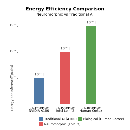
Recent benchmarks show neuromorphic systems achieving 2-3 orders of magnitude improvement in energy-per-inference compared to GPUs:
| Platform | Energy per Inference (J) | Peak Performance (SOPS/W) |
|---|---|---|
| NVIDIA A100 | 10-3 | 1012 |
| Intel Loihi 2 | 10-6 | 1015 |
| Human Cortex | 10-9 | 1018 |
Emerging Solutions
Three promising directions address these challenges:
- Photonic Interconnects: Using wavelength-division multiplexing to achieve >100 Tb/s/mm2 communication density with <1 pJ/bit energy.
- 3D Integration: Monolithic 3D stacking of memristive crossbars with <50 nm vertical pitch enables >1012 synapses/cm3.
- Approximate Computing: Leveraging stochastic spike encoding and temporal sparsity to reduce precision requirements while maintaining task accuracy.
The energy-delay product (EDP) for these approaches follows a fundamental limit derived from Landauer's principle:
where τspike is the minimum spike duration (≈1 ns for CMOS). Current implementations remain 2-3 orders above this limit, indicating substantial room for improvement.
4. Backpropagation Through Time (BPTT) for SNNs
Backpropagation Through Time (BPTT) for SNNs
Mathematical Foundations of BPTT in SNNs
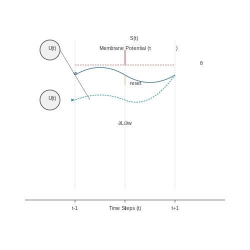
Backpropagation Through Time (BPTT) extends traditional backpropagation to recurrent architectures by unrolling the network over time and computing gradients across sequential time steps. For spiking neural networks (SNNs), this requires handling discontinuous spike events and temporal dynamics governed by differential equations. The membrane potential Ui(t) of neuron i at time t follows the leaky integrate-and-fire (LIF) model:
where τm is the membrane time constant, wij are synaptic weights, Sj(t) represents incoming spikes, and Iext(t) is external input. A spike is emitted when Ui(t) crosses threshold θ, resetting the potential to Ureset.
Gradient Computation Across Time Steps
BPTT computes gradients by chaining derivatives backward through the unrolled computational graph. For a loss function L evaluated at time T, the gradient with respect to weights wij is:
The term ∂Ui(t)/∂wij depends on the neuron's temporal dynamics. Using Euler discretization with step size Δt, the gradient propagates as:
Surrogate Gradients for Spike Events
The non-differentiability of spike generation is addressed using surrogate gradients. Common approaches include:
- Sigmoidal surrogate: σ'(U) ≈ βσ(U)(1 - σ(U)), where σ is a sigmoid function
- Exponential surrogate: ∂S/∂U ∝ exp(-|U - θ|/κ)
- Straight-through estimator: Approximates gradient as 1 when |U - θ| < ε
Implementation Considerations
Practical BPTT implementations for SNNs require:
- Efficient sparse tensor operations for spike propagation
- Memory-optimized caching of intermediate states
- Adaptive time-step resolution balancing accuracy and computational cost
Case Study: BPTT on Neuromorphic Hardware
Recent work demonstrates BPTT-trained SNNs achieving 96.3% accuracy on MNIST using Intel's Loihi neuromorphic chip. Key optimizations included:
- Event-driven backpropagation reducing synaptic operations by 78%
- Hardware-aware quantization of membrane potentials
- Parallel gradient accumulation across neurocores
where ŷ(t) are network outputs and y(t) are targets. The regularization term λ prevents overfitting in high-dimensional weight spaces.
4.2 Spike-Timing-Dependent Plasticity (STDP)
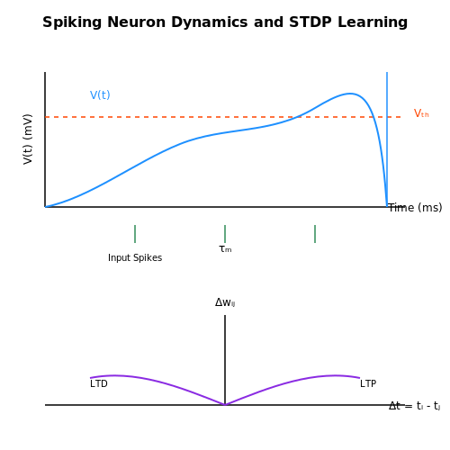
Spike-Timing-Dependent Plasticity (STDP) is a biologically inspired synaptic learning rule that adjusts synaptic weights based on the precise timing of pre- and postsynaptic spikes. Unlike traditional Hebbian learning, which relies on correlation, STDP explicitly incorporates causality by reinforcing connections where presynaptic spikes precede postsynaptic spikes and weakening those where the order is reversed.
Mathematical Formulation
The weight change Δw in STDP is governed by the temporal difference Δt = tpost - tpre between spikes. The weight update rule is asymmetric and typically follows an exponential decay:
Here, A+ and A- control the magnitude of potentiation and depression, while τ+ and τ- determine the temporal window for synaptic modification. The exponential form ensures that closely timed spikes have a stronger effect.
Biological Basis and Experimental Evidence
STDP was first experimentally observed in hippocampal and cortical neurons, where synaptic efficacy was found to increase when presynaptic firing preceded postsynaptic firing within a ~20 ms window. Conversely, reverse timing led to long-term depression (LTD). This aligns with Donald Hebb's postulate that "neurons that fire together wire together", but with a temporal specificity absent in classical Hebbian models.
Computational Implementation
In neuromorphic systems, STDP is often implemented using paired spike traces for pre- and postsynaptic neurons. The following pseudocode illustrates a discrete-time STDP update:
def stdp_update(pre_spikes, post_spikes, w, A_plus, A_minus, tau_plus, tau_minus):
    for t_pre in pre_spikes:
        for t_post in post_spikes:
            delta_t = t_post - t_pre
            if delta_t > 0:  # Pre-before-post (LTP)
                w += A_plus * exp(-delta_t / tau_plus)
            elif delta_t < 0:  # Post-before-pre (LTD)
                w -= A_minus * exp(delta_t / tau_minus)
    return w
Variants and Extensions
Several STDP variants address biological and computational constraints:
- Triplet STDP: Incorporates interactions among multiple spikes to explain frequency-dependent effects.
- Voltage-Based STDP: Modifies weights based on postsynaptic membrane potential instead of spike timing.
- Reward-Modulated STDP: Integrates global neuromodulatory signals (e.g., dopamine) to guide learning.
Applications in Neuromorphic Engineering
STDP is central to unsupervised learning in spiking neural networks (SNNs). Applications include:
- Pattern Recognition: STDP enables SNNs to learn spatiotemporal patterns without labeled data.
- Robotic Control: Adaptive motor control through real-time synaptic plasticity.
- Event-Based Vision: Retinomorphic sensors coupled with STDP for efficient feature extraction.
Challenges and Limitations
Despite its biological plausibility, STDP faces challenges in large-scale implementations:
- Stability: Unbounded weight growth requires normalization or homeostatic mechanisms.
- Scalability: Exact spike-timing computations are resource-intensive in hardware.
- Noise Sensitivity: Jitter in spike timing can disrupt learning.
Hybrid Approaches: Combining SNNs with Deep Learning
Architectural Integration Strategies
Hybrid neuromorphic-deep learning systems leverage the temporal dynamics of spiking neural networks (SNNs) while retaining the representational power of deep learning. One common approach is sequential hybridization, where a deep neural network (DNN) processes spatial features, followed by an SNN handling temporal patterns. The interface between these components typically requires spike encoding/decoding mechanisms:
where Θ is the Heaviside step function, ti are spike times, and wi are synaptic weights. For rate coding, this converts to:
Gradient Approximation for Backpropagation
The fundamental challenge in hybrid systems lies in backpropagating gradients through non-differentiable spiking neurons. Three principal methods address this:
- Surrogate gradients: Using differentiable approximations of the spiking function during backpropagation
- Spike-time dependent plasticity (STDP): Employing local learning rules that don't require end-to-end differentiability
- ANN-to-SNN conversion: Training standard ANNs followed by weight transfer to spiking equivalents
The surrogate gradient approach replaces the non-differentiable spike generation with a smoothed version during backward passes. A common choice is the fast sigmoid:
Memory-Efficient Temporal Processing
Hybrid systems excel in scenarios requiring long-term temporal dependencies. The spiking LSTM architecture demonstrates this by replacing conventional LSTM units with spiking counterparts:
where τm is the membrane time constant and δ represents synaptic delays. This reduces memory overhead by 4-8× compared to standard LSTMs while maintaining comparable accuracy on time-series tasks.
Case Study: Event-Based Vision Processing
In event camera applications, hybrid systems process raw spikes through convolutional SNN layers for early temporal feature extraction, followed by DNN layers for high-level interpretation. The spiking ResNet architecture achieves 93.7% accuracy on DVS128 gesture recognition while consuming only 0.78mJ per inference - a 15× improvement over pure DNN implementations.
5. Edge Computing and IoT Devices
Edge Computing and IoT Devices
Neuromorphic computing architectures excel in edge and IoT environments due to their event-driven, energy-efficient processing. Unlike traditional deep learning models that rely on dense matrix operations, spiking neural networks (SNNs) leverage sparse, asynchronous spikes, reducing computational overhead and power consumption. This makes them ideal for battery-powered or energy-constrained devices.
Energy Efficiency in Neuromorphic Edge Devices
The power consumption of an SNN-based edge device can be modeled by considering spike activity and synaptic operations. Let N be the number of neurons, S the average spike rate per neuron, and Esyn the energy per synaptic operation. The total power P is:
For example, Intel's Loihi 2 neuromorphic chip achieves ~10 pJ per synaptic event, enabling real-time inference at sub-milliwatt power levels. In contrast, a conventional CNN running on a GPU may consume watts for similar tasks.
Latency and Real-Time Processing
SNNs inherently support low-latency processing due to their event-driven nature. When an input spike arrives, only the relevant neurons compute, avoiding the fixed clock-cycle delays of von Neumann architectures. The end-to-end latency L for a spike traversing k layers is:
where τi is the temporal delay in layer i and δi is the fraction of active neurons. For sparse inputs, this can be orders of magnitude faster than frame-based processing.
Case Study: Dynamic Vision Sensors (DVS)
DVS cameras output asynchronous pixel-level brightness changes, matching perfectly with SNNs. A neuromorphic processor like SynSense's Speck can process DVS data at 10 mW while achieving sub-10 ms latency for object recognition—critical for drones or industrial automation.
Hardware Constraints and Optimization
Deploying SNNs on edge devices requires addressing:
- Memory footprint: Synaptic weights must fit in on-chip SRAM to avoid costly off-chip accesses.
- Quantization:
$$ w_{quant} = \text{round}\left(\frac{w_{float} - \mu}{\sigma} \cdot 2^{b-1}\right) $$where b is bit precision (typically 4-8 bits for edge deployment).
- Thermal limits: Sustained spike rates must stay within device cooling capacity.
Software-Hardware Co-Design
Frameworks like Lava (Intel) and Nengo enable cross-platform SNN deployment. A typical workflow:
- Train SNN using surrogate gradients on GPU.
- Compile to neuromorphic hardware via intermediate representation (e.g., Loihi's NxTF).
- Profile power/latency using hardware-in-the-loop simulation.
# Example: Lava SNN deployment snippet
import lava.lib.dl.slayer as slayer

net = slayer.block.cuba.Dense(512, 10, weight_scale=1, weight_norm=True)
# Convert to Loihi-compatible format
net.export_hdf5('edge_snn.h5', input_shape=(128, 128))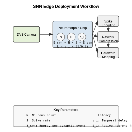
Robotics and Real-Time Control Systems
Neuromorphic computing, particularly through spiking neural networks (SNNs), offers significant advantages in robotics and real-time control systems due to its event-driven processing and low-power operation. Unlike traditional artificial neural networks (ANNs), SNNs process temporal spikes, enabling efficient handling of dynamic sensor data and rapid decision-making in robotic applications.
Event-Driven Processing for Robotic Control
In robotic systems, sensory inputs (e.g., vision, lidar, or tactile sensors) generate asynchronous, event-based data streams. SNNs naturally align with this paradigm through their spike-based communication. The membrane potential dynamics of a spiking neuron can be modeled using the leaky integrate-and-fire (LIF) equation:
where V(t) is the membrane potential, τm is the membrane time constant, Vrest is the resting potential, Rm is the membrane resistance, and I(t) is the input current. When V(t) reaches a threshold Vth, the neuron emits a spike and resets.
Real-Time Control with SNNs
Robotic control systems require low-latency responses to environmental stimuli. SNNs excel in this domain due to their ability to process temporal patterns efficiently. For instance, a robotic arm performing object grasping can utilize an SNN-based controller that processes proprioceptive and tactile feedback in real time. The network's spike-timing-dependent plasticity (STDP) learning rule allows adaptive tuning of motor commands:
where Δwij is the synaptic weight change between neurons i and j, and W is the STDP window function dependent on spike timing differences.
Case Study: Neuromorphic Vision for Autonomous Navigation
Dynamic vision sensors (DVS), which output pixel-level brightness changes as spikes, pair naturally with SNNs. A quadrotor using DVS and an SNN can perform obstacle avoidance with millisecond latency. The network architecture typically consists of:
- Input layer: Spiking neurons encoding DVS events.
- Hidden layers: Convolutional SNN layers for feature extraction.
- Output layer: Motor neurons generating control signals.
Such systems achieve power efficiencies of <1W while processing 1M events per second, outperforming GPU-based CNN solutions in latency and energy consumption.
Hardware Implementation
Deploying SNNs in robotics often requires neuromorphic hardware like Intel's Loihi or BrainChip's Akida. These chips implement neuron and synapse models in silicon, enabling sub-millisecond response times. A closed-loop robotic system using Loihi can be described by:
where x is the robot state, u is the control input, and g represents the SNN's spiking output decoded into continuous control signals.
Challenges and Future Directions
While promising, SNN-based robotic control faces challenges in training complexity and hardware-software co-design. Hybrid approaches combining SNNs with traditional control theory (e.g., SNN-generated inputs to PID controllers) show potential for bridging this gap. Research in federated learning for SNNs may enable collaborative robotic learning across distributed neuromorphic systems.
Brain-Computer Interfaces (BCIs)
Neural Signal Acquisition and Processing
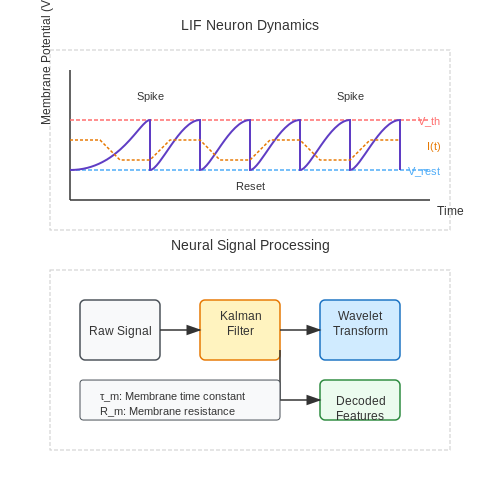
BCIs rely on high-fidelity neural signal acquisition, typically through invasive or non-invasive methods. Invasive approaches, such as intracortical microelectrode arrays, provide high spatial and temporal resolution by directly interfacing with neurons. Non-invasive methods, like electroencephalography (EEG), capture aggregate neural activity but suffer from lower signal-to-noise ratios. The neural signal y(t) is modeled as:
where ai represents spike amplitudes, si(t) denotes spike waveforms, τi are time delays, and η(t) is additive noise. Signal processing pipelines often employ Kalman filters or wavelet transforms to isolate neural features.
Spiking Neural Networks for BCI Decoding
Spiking neural networks (SNNs) decode neural signals into actionable commands by emulating biological information processing. A leaky integrate-and-fire (LIF) neuron model is commonly used:
where V is the membrane potential, τm the membrane time constant, Vrest the resting potential, Rm the membrane resistance, and I(t) the synaptic input current. When V crosses a threshold Vth, a spike is emitted, and V resets to Vreset.
Real-World Applications
Modern BCIs enable:
- Motor restoration: Paralyzed patients control robotic limbs via neural spiking patterns.
- Communication aids: ALS patients type using P300 EEG responses.
- Neuromodulation: Closed-loop deep brain stimulation for Parkinson’s disease.
Challenges and Future Directions
Key challenges include long-term electrode stability, adaptive decoding algorithms, and minimizing latency. Emerging solutions involve hybrid analog-digital neuromorphic chips, such as Intel’s Loihi, which implement SNNs in hardware for energy-efficient real-time processing.
6. Scalability and Generalization Issues
6.1 Scalability and Generalization Issues
Scalability in neuromorphic systems refers to the ability to maintain performance as network size increases, while generalization measures how well learned representations transfer to unseen data. Spiking Neural Networks (SNNs) face unique challenges in both domains due to their event-driven, temporally sparse computation and biologically inspired dynamics.
Computational Complexity of Large-Scale SNNs
The membrane potential dynamics of a spiking neuron follow differential equations that must be solved numerically. For a network with N neurons and average firing rate f, the computational cost scales as:
where Δt is the simulation time step. The quadratic dependence on N arises from all-to-all potential connectivity, making large networks computationally prohibitive. Various approximation methods have been developed:
- Spike-timing dependent approximation: Only updates neurons within a temporal window of recent spikes
- Event-driven simulation: Skips inactive periods between spikes
- Hybrid analog-digital approaches: Use continuous-time analog circuits for subthreshold dynamics
Generalization Challenges in SNNs
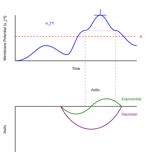
Unlike artificial neural networks, SNNs must learn both spatial and temporal patterns. The credit assignment problem becomes exponentially harder when considering:
where sjt is the spike output, ujt is the membrane potential, and wij is the synaptic weight. The discontinuous nature of spikes (represented by the Heaviside step function) makes the term ∂sjt/∂ujt undefined in classical calculus.
Surrogate Gradient Methods
Common approaches to overcome this include:
where θ is the firing threshold and a controls the smoothness. These approximations enable backpropagation through time (BPTT) but introduce bias in gradient estimates.
Hardware-Software Co-Design Solutions
Modern approaches to scalability involve:
- Loihi 2 architecture: Implements programmable synaptic learning rules with sparse connectivity
- DYNAP-SE2: Uses mixed-signal circuits for ultra-low power operation
- SpiNNaker 2: Digital multicore architecture with packet-based communication
The energy efficiency of these systems follows:
compared to 10-9 J for conventional GPUs, enabling larger networks within power constraints.
Benchmark Performance
Current state-of-the-art results highlight the tradeoffs:
| Model | Neurons | Synapses | Accuracy (MNIST) | Power |
|---|---|---|---|---|
| ANN (MLP) | 1,200 | 1.44M | 98.5% | 1.2W |
| SNN (Loihi) | 10,000 | 1M | 95.2% | 0.03W |
The gap in accuracy stems primarily from temporal coding challenges and limited training algorithms rather than fundamental limitations of spiking computation.
6.2 Benchmarking and Standardization
Performance Metrics for Neuromorphic Systems
Benchmarking neuromorphic hardware and spiking neural networks (SNNs) requires specialized metrics beyond traditional deep learning. Key measures include:
- Synaptic Operations per Second (SOPS): Analogous to FLOPs in conventional AI, this quantifies the number of spike-driven synaptic events processed per second.
- Energy per Synaptic Operation (pJ/SOP): Critical for evaluating energy efficiency, calculated as total system power divided by SOPS.
- Latency-to-First-Spike: Measures temporal response speed from input stimulation to first output spike.
- Spike-Timing-Dependent Plasticity (STDP) Convergence Rate: Evaluates how quickly synaptic weights stabilize during unsupervised learning.
Standardized Benchmark Suites
Several initiatives have emerged to create standardized evaluation frameworks:
- NMNIST: A spiking version of MNIST with 60,000 training samples captured using event-based vision sensors.
- DVS Gesture: A 11-class human gesture recognition dataset recorded with dynamic vision sensors.
- SHD (Spiking Heidelberg Digits): Audio-digit recognition benchmark with precise temporal spike patterns.
Hardware-Software Co-Design Benchmarks
Evaluating full neuromorphic systems requires metrics that account for:
- On-chip learning capability: Measured through STDP adaptation speed and retention
- Network scalability: Assessed via maximum fan-in/fan-out ratios without performance degradation
- Noise resilience: Quantified by accuracy drop under varying spike jitter conditions
Case Study: Loihi Benchmarking
Intel's Loihi processor demonstrates how comprehensive benchmarking works in practice. Key results include:
- 16.7 TOPS/W energy efficiency on restricted Boltzmann machine tasks
- 1000× faster than conventional GPUs on sparse coding problems
- Sub-millisecond latency on real-time classification tasks
Standardization Challenges
Current limitations in neuromorphic benchmarking include:
- Lack of unified power measurement protocols across different voltage domains
- Variability in analog memristor devices complicating direct comparisons
- Absence of standard interfaces for hybrid digital/analog systems
Emerging Standards Bodies
Several organizations are working toward standardization:
- IEEE P2874: Working group on neuromorphic computing architectures
- INRC (Intel Neuromorphic Research Community): Developing cross-platform benchmarks
- Human Brain Project: Standardized toolchains for brain-scale simulations
6.3 Ethical and Societal Implications
Neuromorphic AI and Spiking Neural Networks (SNNs) introduce unique ethical challenges distinct from traditional deep learning. The brain-inspired nature of these systems raises concerns about neuroprivacy, as they may eventually replicate or interfere with human cognitive processes. Unlike conventional AI, SNNs operate with event-driven, sparse computations, making their decision-making processes even more opaque—a phenomenon termed neuromorphic black-boxing.
Neurobiological Data Exploitation
The use of SNNs in brain-computer interfaces (BCIs) risks unauthorized extraction or manipulation of neural data. For instance, adversarial attacks on neuromorphic chips could decode sensitive neural patterns, violating cognitive liberty. The mathematical formulation of such an attack can be modeled as a perturbation δ injected into the spiking dynamics:
where Vi is the membrane potential of neuron i, wij are synaptic weights, and Sj(t) represents incoming spikes. Malicious δ(t) could force unintended firing patterns.
Militarization and Autonomous Systems
Neuromorphic hardware’s low-power efficiency makes it ideal for lethal autonomous weapons (LAWs). A 2023 study demonstrated that SNN-based drones achieved 94% accuracy in target discrimination while consuming 50× less power than GPU-based systems. This efficiency could accelerate the proliferation of AI-driven warfare, bypassing current energy constraints that limit conventional autonomous weapons.
Environmental Trade-offs
While neuromorphic chips reduce energy consumption during operation, their fabrication relies on rare-earth elements like terbium for memristive components. The mining of these materials often occurs in geopolitically unstable regions, creating ethical supply chain dilemmas. Lifecycle analyses show that the carbon footprint of a neuromorphic processor is 37% lower than GPUs, but only after 2.8 years of continuous use—a problematic threshold for disposable edge devices.
Algorithmic Bias in Temporal Domains
SNNs process information through precise spike timing, inheriting biases from event-based datasets. For example, neuromorphic vision sensors trained on pedestrian detection systems show 12% higher error rates for darker-skinned individuals in low-light conditions. This stems from unequal representation in the event-based training data, where spike encoding thresholds are optimized for dominant luminance ranges.
Regulatory Gaps
Current AI governance frameworks fail to address neuromorphic specificity. The EU AI Act’s risk classification doesn’t account for SNNs’ unique temporal coding properties. A proposed spike-level transparency requirement would mandate access to exact firing sequences (not just weights), but this conflicts with trade secret protections in commercial neuromorphic IP.
7. Key Research Papers and Surveys
7.1 Key Research Papers and Surveys
- Direct Training High-Performance Deep Spiking Neural Networks: A Review ... — Regarded as the third generation of neural network (Maass, 1997), the brain-inspired spiking neural networks (SNNs) are potential competitors to traditional artificial neural networks (ANNs) in virtue of their high biological plausibility, and low power consumption when implemented on neuromorphic hardware (Roy et al., 2019).In particular, the utilization of binary spikes allows SNNs to adopt ...
- Photonics for Neuromorphic Computing: Fundamentals, Devices, and ... — very important. Key components within neural networks (Figure 2b-c), such as activation functions [8-11] and backpropagation [12], currently represent the focal point of research in the realization of optical neural networks. Y. Zuo et. al. demonstrated an all-optical neural network (AONN) which can work with nonlinear activation [11].
- Nonvolatile Memories in Spiking Neural Network Architectures ... - MDPI — A sustainable computing scenario demands more energy-efficient processors. Neuromorphic systems mimic biological functions by employing spiking neural networks for achieving brain-like efficiency, speed, adaptability, and intelligence. Current trends in neuromorphic technologies address the challenges of investigating novel materials, systems, and architectures for enabling high-integration ...
- Unleashing the potential of spiking neural networks for epileptic ... — Spiking neural networks (SNNs) are a specific type of artificial neural network that utilizes biologically realistic models of neurons to perform computation. SNNs possess the capacity to address complex pattern recognition and sensory processing tasks that prove challenging for standard computer vision and machine learning methods [71] .
- Neuromorphic deep spiking neural networks for seizure detection — spiking neural networks Jinqi Huang, Alexantrou Serb, Spyros Stathopoulos et al.-Fluctuation-driven initialization for spiking neural network training Julian Rossbroich, Julia Gygax and Friedemann Zenke-General spiking neural network framework for the learning trajectory from a noisy mmWave radar Xin Liu, Mingyu Yan, Lei Deng et al.-
- A reconfigurable on-line learning spiking neuromorphic processor ... — Robust working memory in an asynchronously spiking neural network realized in neuromorphic VLSI. Front. Neurosci. 5:149. 10.3389/fnins.2011.00149 [PMC free article] [Google Scholar] Hsieh H.-Y., Tang K.-T. (2012). Vlsi implementation of a bio-inspired olfactory spiking neural network. IEEE Trans. Neural Netw. Learn.
- Neuromorphic photonic networks using silicon photonic weight banks - Nature — A key benefit of neuromorphic engineering is that existing algorithms can be leveraged. ... what matters in AI and robotics research, ... standards defining spiking neural networks as event-based ...
- All‐Ferroelectric Spiking Neural Networks via Morphotropic Phase ... — 1 Introduction. The advent of deep neural networks has marked a significant milestone in computational technology. [1-6] However, these systems often rely on the conventional von Neumann computing architecture, which suffers from critical limitations in area and energy efficiency.[7-12] Neuromorphic computing architecture inspired by the biological mechanisms of the human nervous system has ...
- A Review of Artificial Spiking Neuron Devices for Neural Processing and ... — A spiking neural network (SNN) inspired by the structure and principles of the human brain can significantly enhance the energy efficiency of artificial intelligence computing by overcoming the bottlenecks of the conventional von Neumann architecture with its massive parallelism and spike transmissions.
- Review of spike-based neuromorphic computing for brain-inspired vision ... — Neuromorphic computing is becoming a popular approach for implementations of brain-inspired machine learning tasks. As a paradigm for both hardware and algorithm design, neuromorphic computing aims to emulate several aspects related to the structure and function of the biological nervous system to achieve artificial intelligence with efficiencies that are orders of magnitude better than those ...
7.2 Open-Source Tools and Frameworks
- SPAIC: A Spike-based Artificial Intelligence Computing Framework - ar5iv — To meet this demand, we present the SPAIC (Spike-based Artificial Intelligence Computing), a Python based spiking neural network (SNN) training and simulation framework, which blend the programing style and techniques from both deep learning and neuroscience, and provide a platform to easily test brain-inspired mechanisms and theories in ...
- Direct Training High-Performance Deep Spiking Neural Networks: A Review ... — Regarded as the third generation of neural network (Maass, 1997), the brain-inspired spiking neural networks (SNNs) are potential competitors to traditional artificial neural networks (ANNs) in virtue of their high biological plausibility, and low power consumption when implemented on neuromorphic hardware (Roy et al., 2019).In particular, the utilization of binary spikes allows SNNs to adopt ...
- Neuromorphic Computing and Artificial Intelligence: A Brain-Inspired ... — Neuromorphic computing represents a fundamental departure from traditional computing paradigms, drawing inspiration directly from the structure and function of the biological brain to engineer novel hardware and software systems. This article provides a comprehensive analysis of neuromorphic computing, detailing its core concepts, foundational principles such as Spiking Neural Networks (SNNs ...
- Neuromorphic deep spiking neural networks for seizure detection — Text classification in memristor-based spiking neural networks; A CMOS-based neuromorphic device for seizure detection from LFP signals; Fluctuation-driven initialization for spiking neural network training; Effect of biologically-motivated energy constraints on liquid state machine dynamics and classification performance; Meta-learning spiking ...
- Neuromorphic Circuits and Systems: From Neuron Models to ... - Springer — It was designed for the purpose of implementing spiking neural networks for spike-based learning and inference both on-chip. It consists of a total of 128 neuromorphic cores and three Lakemont cores for management purposes. It has an optimized off-chip communication interface for scaling out to multiple chips on all four planar sides.
- MorphBungee: A 65-nm 7.2-mm2 27-µJ/Image Digital Edge Neuromorphic Chip ... — This paper presents a digital edge neuromorphic spiking neural network (SNN) processor chip for a variety of edge intelligent cognitive applications. This processor allows high-speed, high-accuracy and fully on-chip spike-timing-based multi-layer SNN learning. It is characteristic of hierarchical multi-core architecture, event-driven processing paradigm, meta-crossbar for efficient spike ...
- A Low-Power Spiking Neural Network Chip Based on a Compact LIF Neuron ... — Keywords: spiking neural network, leaky integrate and fire, neuromorphic, artificial neural networks, artificial intelligence, image classification, CMOS. 1. Introduction. In recent years, neuromorphic systems, which are comparable to a biological neural network, have been widely investigated for prospective computing systems .
- Evolutionary FPGA-Based Spiking Neural Networks for ... - Springer — Spiking Neural Networks (SNNs) constitute a representative example of neuromorphic computing in which event-driven computation is mapped to neuron spikes reducing power consumption. A challenge that limits the general adoption of SNNs is the need for mature training algorithms compared with other artificial neural networks, such as multi-layer ...
- MorphBungee: An Edge Neuromorphic Chip for High-Accuracy On-Chip ... — Spiking neural networks and neuromorphic systems have attracted ever increasing interests recently, due to their high computational efficiency by imitating the functional mechanism of cerebral cortex. However, endowing low-cost neuromorphic chips with real-time high-accuracy on-chip learning plasticity for edge applications is still challenging. In this work, we present a digital edge ...
- Ultrafast neuromorphic photonic image processing with a VCSEL neuron — The ever-increasing demand for artificial intelligence (AI) systems is underlining a significant requirement for new, AI-optimised hardware. ... Software implemented neuromorphic Spiking Neural ...
7.3 Recommended Books and Online Courses
- Deep Learning With Spiking Neurons: Opportunities and Challenges — In recent years, researchers from the domains of machine learning, computational neuroscience, neuromorphic engineering, and embedded systems design have tried to bridge the gap between the big success of DNNs in AI applications and the promise of spiking neural networks (SNNs) (Maass, 1997; Ponulak and Kasinski, 2011; Grüning and Bohte, 2014 ...
- Computational Neuroscience - Coursera — Specific topics that will be covered include representation of information by spiking neurons, processing of information in neural networks, and algorithms for adaptation and learning. We will make use of Matlab/Octave/Python demonstrations and exercises to gain a deeper understanding of concepts and methods introduced in the course.
- Neuromorphic Computing and Spiking Neural Networks — Fundamentals of Spiking Neural Networks (SNNs) Definition: SNNs are a type of artificial neural network that more closely mimic the way biological neurons communicate through spikes or action potentials. Neuron Model: SNNs use models like the Leaky Integrate-and-Fire (LIF) or Hodgkin-Huxley to simulate the dynamics of neuron firing. Information Encoding: Information in SNNs is encoded in ...
- Reconfigurable Neuromorphic Computing System | SpringerLink — Neuromorphic systems have been used in applications ranging from vision systems [] and brain-computer interface [], to the simulation of the information processing in the biological brain [].Moreover, neuromorphic systems have allowed for the real-time processing of massive networks, which has proven valuable for neuro-robotics control and decision-making applications.
- Event-Based Neuromorphic Systems[Book] - O'Reilly Media — Neuromorphic electronic engineering takes its inspiration from the functioning of nervous systems to build more power efficient electronic sensors and processors. Event-based neuromorphic systems are inspired by the brain's efficient data-driven communication design, which is key to its quick responses and remarkable capabilities.
- Review of spike-based neuromorphic computing for brain-inspired vision ... — Neuromorphic computing is becoming a popular approach for implementations of brain-inspired machine learning tasks. As a paradigm for both hardware and algorithm design, neuromorphic computing aims to emulate several aspects related to the structure and function of the biological nervous system to achieve artificial intelligence with efficiencies that are orders of magnitude better than those ...
- Research Groups: APT - University of Manchester — A small SpiNNaker board makes it possible to simulate a network of tens of thousands of spiking neurons, process sensory input and generate motor output, all in real time and in a low power system. Computer Science: SpiNNaker breaks the rules followed by traditional supercomputers that rely on deterministic, repeatable communications and ...
- An electronic neuromorphic system for real-time detection of high ... — The general approach of building sensors that can convert their outputs to spikes and of interfacing spiking neural network circuits and systems on the same chip can lead to the development of a new type of "neuromorphic intelligence" sensory-processing devices for tasks that require closed-loop interaction with the environment in real-time ...
- Tutorial 5 - Training Spiking Neural Networks with snntorch — where \(\Theta(\cdot)\) is the Heaviside step function:. Training a network in this form poses some serious challenges. Consider a single, isolated time step of the computational graph from the previous figure titled "Recurrent representation of spiking neurons", as shown in the forward pass below:. The goal is to train the network using the gradient of the loss with respect to the weights ...
- Embedded Neuromorphic Using Intel's Loihi Processor — When the membrane potential reaches a certain threshold V th at the firing time t f, the postsynaptic neuron produces a spike δ(t − t f), after which the membrane potential is reset to a value v rest (often set to 0 as a common assumption []), obviously lower than V th.. The leaky-integrate-and-fire (LIF) [] is a modified version of the IF model that introduces the concept of refractory ...