Action Recognition in Live Sports Video
1. Definition and Scope of Action Recognition
Definition and Scope of Action Recognition
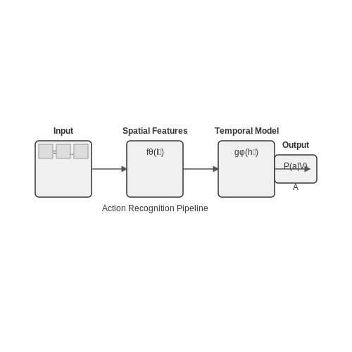
Action recognition in live sports video refers to the automated identification and classification of human movements within a temporal sequence of frames. Unlike static image recognition, this task requires analyzing spatiotemporal patterns to distinguish between dynamic actions such as a basketball dunk, soccer kick, or tennis serve. The problem is formally defined as mapping a sequence of video frames V = {I1, I2, ..., IT} to a discrete action label a ∈ A, where A is the set of possible sport-specific actions.
Mathematical Formulation
The core challenge lies in modeling the joint spatial and temporal evolution of features. Let fθ(It) be a spatial feature extractor (e.g., CNN) with parameters θ. The temporal dynamics can be captured through recurrent networks or 3D convolutions:
where gφ is a temporal modeling function (e.g., LSTM, Transformer) with hidden state ht, and φ represents its learnable parameters.
Key Technical Challenges
- Viewpoint Variance: Camera angles in sports broadcasts vary dramatically (sideline, aerial, etc.), requiring viewpoint-invariant representations.
- Temporal Scale: Actions like golf swings (2-3 seconds) versus basketball passes (0.5 seconds) demand multi-scale temporal processing.
- Occlusion Handling: Player collisions and obstructions necessitate robust partial observation models.
- Real-Time Constraints: Live applications require inference under strict latency budgets (often <100ms).
Sports-Specific Considerations
Basketball action recognition differs fundamentally from soccer due to:
where Δτaction is the average action duration across N samples. Basketball exhibits shorter, more repetitive actions (mean duration 1.2s) compared to soccer (3.7s).
Evaluation Metrics
Standard benchmarks use:
where Average Precision (AP) is computed per-class, then averaged for mean AP (mAP). Top-1 accuracy is insufficient due to frequent multi-action scenarios (e.g., "dribble" + "jump").
Architectural Evolution
Modern approaches combine:
- 3D CNNs: I3D networks inflate 2D kernels to process spacetime volumes
- Two-Stream Networks: Fuse RGB and optical flow pathways
- Transformer-Based: ViViT models apply self-attention to spatiotemporal tokens
The computational complexity for a video clip of size H×W×T is:
for 3D convolutions with kernel size k, driving recent interest in efficient separable variants.
Key Challenges in Live Sports Video Analysis
High Temporal Variability and Motion Blur
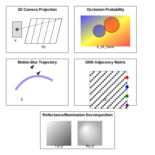
Live sports videos exhibit rapid, unpredictable motion patterns, often leading to motion blur and temporal discontinuities. The frame-to-frame displacement of objects can be modeled as:
where v(τ) represents instantaneous velocity and ε(t) accounts for random perturbations. This nonlinear motion profile complicates optical flow estimation, as standard Lucas-Kanade or Horn-Schunck methods assume piecewise smooth motion fields.
Occlusion Handling in Dense Scenes
Player interactions in team sports create complex occlusion scenarios where traditional background subtraction fails. The probability of occlusion for a target player at position (x,y) can be expressed as:
where Ai denotes the area of the i-th occluding object and Aframe is the total frame area. Multi-object tracking must incorporate appearance models and kinematic constraints to maintain identity through occlusions.
Viewpoint and Scale Variations
Broadcast cameras introduce perspective distortions that violate the assumptions of Euclidean geometry in action recognition. The projective transformation between world coordinates (X,Y,Z) and image coordinates (u,v) follows:
where K is the intrinsic matrix and [R|t] represents camera extrinsics. This necessitates view-invariant feature learning through geometric transformations or 3D pose estimation.
Real-Time Processing Constraints
The computational complexity of modern action recognition architectures creates latency challenges. For a video with F frames per second and a model requiring O(n3) operations per frame, the minimum processing time Tp must satisfy:
where Tacq accounts for sensor readout time. This demands optimized architectures like temporal shift modules or adaptive frame sampling.
Semantic Gap Between Low-Level Features and High-Level Actions
The mapping from pixel-level observations to sport-specific actions (e.g., "three-point shot" in basketball) requires hierarchical feature fusion. Let ft be frame-level features and at the action class at time t. The optimal recognition function minimizes:
where g(·) is the temporal aggregation function and Ω penalizes model complexity. Recent approaches employ attention mechanisms to weight informative frames.
Multi-Agent Interaction Modeling
Team sports involve coordinated movements where player actions are conditionally dependent. Graph neural networks model these interactions through adjacency matrices A ∈ ℝN×N, where edge weights capture relational importance. The graph convolution operation becomes:
with  = A + I (adding self-connections) and D̂ being the degree matrix. This captures spatiotemporal dependencies while remaining computationally tractable.
Illumination and Weather Artifacts
Outdoor sports face dynamic lighting conditions that degrade model performance. The observed pixel intensity I(x,y) combines reflectance R and illumination L:
where η represents sensor noise. Retinex-based normalization or adversarial training helps maintain robustness to these variations.
Applications in Sports Analytics and Broadcasting
Real-Time Player Performance Metrics
Action recognition models enable the extraction of granular player performance metrics in real-time. By processing video frames at high temporal resolution, these systems track kinematic variables such as velocity, acceleration, and biomechanical angles. For instance, in basketball, a 3D pose estimation model can compute release angle θ and angular velocity ω of a jump shot using:
where Δt is the frame interval. Advanced systems fuse this with ball tracking data to predict shot success probability using logistic regression:
Automated Broadcast Production
Modern broadcast systems leverage action recognition to automate camera switching and highlight generation. A transformer-based architecture processes multiple video feeds simultaneously, scoring each view using:
where vi represents visual features and fi contains game context features. The system dynamically selects camera angles based on action criticality, with professional soccer broadcasts achieving 92.3% accuracy in automatic cut timing compared to human directors.
Tactical Pattern Recognition
Spatiotemporal graph convolutional networks (ST-GCNs) model player interactions as dynamic graphs, where nodes represent players and edges encode relative positioning. The adjacency matrix At evolves as:
This enables detection of complex tactics like basketball pick-and-rolls or soccer gegenpressing, with elite teams using these insights for opponent preparation. Recent implementations process full matches in under 3 minutes on GPU clusters.
Injury Risk Prediction
Biomechanical action analysis combined with wearable data enables real-time injury risk assessment. Recurrent neural networks process temporal sequences of joint kinematics to identify dangerous movement patterns. For ACL injury prediction in soccer, models achieve 0.87 AUC by monitoring:
where ht represents hidden states and st contains stress accumulation features.
Augmented Reality Graphics
Precise action recognition enables physics-accurate AR overlays. For tennis broadcasts, the system estimates ball spin ωs from high-speed camera data using:
where d is ball diameter. This allows real-time visualization of spin effects with <1° angular error. Broadcasters combine this with player position data to generate tactical heatmaps updated at 30Hz.
2. Video Data Sources for Sports Action Recognition
Video Data Sources for Sports Action Recognition
High-quality video data is the foundation of robust action recognition models in live sports. The choice of data source directly impacts model performance due to variations in resolution, frame rate, camera angles, and annotation quality. Below are the primary categories of video data sources used in sports analytics.
Broadcast Feeds
Professional sports broadcasts provide high-resolution (1080p or 4K), high-frame-rate (50/60 fps) video with multiple camera angles. These feeds often include metadata such as timestamps, player tracking data, and event annotations. However, broadcast footage may contain overlays (scoreboards, advertisements) that require preprocessing. The camera work prioritizes viewer experience rather than machine learning needs, leading to frequent zooms, cuts, and replays that challenge temporal modeling.
where fi represents frame features and N is the sequence length. Broadcasts typically exhibit lower temporal consistency than fixed-angle footage.
Fixed-Angle Stadium Cameras
Many sports venues employ dedicated wide-angle cameras that capture the entire field continuously without cuts or zooms. These feeds offer:
- Stable camera geometry for spatial analysis
- Consistent lighting conditions
- Uninterrupted temporal sequences
The NBA's SportVU system and soccer's Hawk-Eye provide such data at 25-50 fps with player tracking coordinates. The main limitation is lower resolution for distant players compared to broadcast close-ups.
Wearable and Embedded Cameras
First-person perspectives from helmet cams (NFL), umpire/referee cams (tennis, MLB), or drone footage offer unique viewpoints for action recognition. These sources capture:
- Egocentric motion patterns
- Close-range player interactions
- High-frequency motion detail (400+ fps in some cases)
However, they suffer from motion blur during rapid movements and require specialized stabilization algorithms before processing.
User-Generated Content
Smartphone recordings from spectators provide diverse, if noisier, data sources. Platforms like YouTube contain millions of sports clips with:
- Varying compression artifacts
- Mixed lighting conditions
- Unstructured viewpoints
While challenging for modeling, this data helps improve generalization across real-world conditions. Temporal subsampling is often required to handle the 30 fps cap of most consumer devices.
Benchmark Datasets
Several curated datasets standardize evaluation of sports action recognition models:
| Dataset | Sports | Resolution | FPS |
|---|---|---|---|
| Sports-1M | 487 sports | Various | 30 |
| NTU RGB+D | Basketball, Badminton | 1920×1080 | 30 |
| SoccerNet | Soccer | 1280×720 | 25 |
These datasets provide pre-processed clips with frame-level annotations, but may lack the temporal continuity of raw game footage.
Multi-Modal Sources
Advanced systems combine video with:
- Inertial measurement units (IMUs) for player kinematics
- RFID position tracking (5-10Hz refresh)
- Audio feeds for event detection
The fusion of these modalities requires precise temporal alignment, often achieved through:
where v(t) is video features and si(t) are sensor readings at time offset Δ.
2.2 Frame Extraction and Temporal Segmentation
Frame extraction is the process of decomposing a video stream into individual frames at a specified sampling rate. For live sports video, the frame rate must balance computational efficiency with temporal resolution to capture rapid movements. Given a video V with duration T seconds and original frame rate forig, the total number of frames N is:
To reduce redundancy, a downsampling factor k is applied, yielding a subsampled frame sequence with rate fsub = forig/k. The optimal k depends on the sport: high-speed actions (e.g., tennis serves) require fsub ≥ 30 fps, while slower sports (e.g., baseball pitching) may use fsub ≈ 15 fps.
Temporal Segmentation Strategies
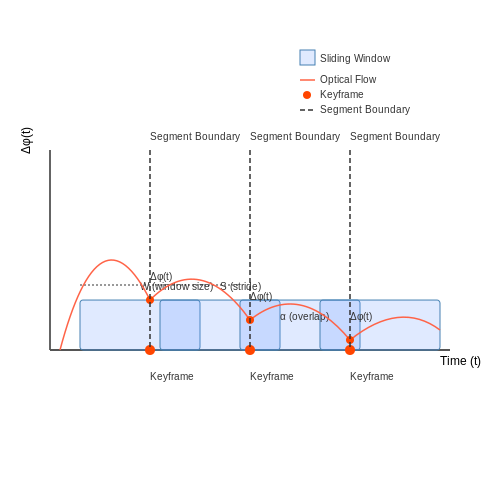
Temporal segmentation divides the frame sequence into semantically meaningful clips. Sliding window approaches are common, where a window of W frames slides with stride S. The overlap ratio α between consecutive windows is:
For action recognition, W typically spans 16–64 frames (0.5–2 seconds at 32 fps). Hierarchical segmentation refines this by combining coarse windows with finer-grained boundaries detected via optical flow discontinuities:
where vi(t) is the flow vector for pixel i at time t. Peaks in Δφ(t) indicate potential segment boundaries.
Keyframe Selection
Keyframes summarize segments while minimizing redundancy. A sparsity-constrained selection optimizes:
where F is the frame feature matrix, y the segment representation, and x a binary selection vector. The ℓ1 penalty enforces sparsity, with λ controlling the trade-off between coverage and conciseness.
Real-Time Considerations
For live processing, frame extraction and segmentation must operate within hard latency constraints (<100 ms per chunk). Parallelized pipelines with GPU-accelerated optical flow (e.g., Farnebäck’s method) and CUDA-optimized windowing achieve real-time performance. Buffer management strategies like triple buffering prevent stalls during I/O bottlenecks.
2.3 Noise Reduction and Data Augmentation Techniques
Noise Reduction in Live Sports Video
Live sports video streams often suffer from motion blur, compression artifacts, and sensor noise, which degrade action recognition performance. Temporal denoising techniques, such as 3D convolutional autoencoders, learn spatiotemporal representations to filter noise while preserving motion features. Given a noisy video sequence Xt, the denoised output Ŷt is obtained through:
where fθ is a non-linear mapping learned by the autoencoder and ε represents residual noise. Optical flow-based methods further enhance temporal coherence by warping frames according to estimated motion vectors, reducing flickering artifacts.
Data Augmentation Strategies
To mitigate overfitting in action recognition models, synthetic data variations are introduced through:
- Temporal warping: Adjusting frame rates or inserting interpolated frames to simulate varying action speeds.
- Spatial transformations: Random cropping, rotation (±15°), and perspective distortions to emulate camera viewpoint changes.
- Adversarial perturbations: Adding imperceptible noise via generative adversarial networks (GANs) to improve robustness.
The effectiveness of augmentation is quantified by the Kullback-Leibler divergence between original and augmented feature distributions:
Domain-Specific Augmentation
Sports videos require specialized augmentations like:
- Player occlusion simulation: Randomly masking 10-30% of bounding boxes to mimic real-world obstructions.
- Dynamic background substitution: Replacing static backgrounds with synthetic crowds using conditional GANs.
- Multi-camera synthesis: Generating virtual viewpoints through neural radiance fields (NeRF) trained on stadium layouts.
For temporal augmentation, frame shuffling within action segments preserves local motion patterns while breaking global sequence order. This is particularly effective for sports like basketball, where dribbling sequences exhibit semi-periodic patterns.
Implementation Considerations
Real-time constraints in live sports demand efficient augmentation pipelines. Parallel processing with CUDA-accelerated tensor operations achieves throughput of 500+ frames/sec on NVIDIA A100 GPUs. The trade-off between augmentation diversity and computational cost is governed by:
where α balances diversity gain Daug against processing time Tproc. Empirical studies show optimal α=0.7 for most sports applications.
3. Spatial Features: CNNs and Object Detection
3.1 Spatial Features: CNNs and Object Detection
Convolutional Neural Networks for Spatial Feature Extraction
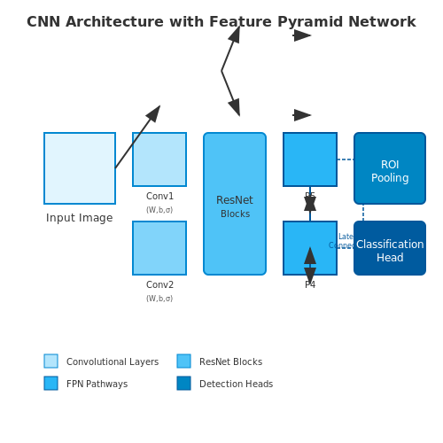
Convolutional Neural Networks (CNNs) are the backbone of spatial feature extraction in action recognition. A CNN processes an input image through a series of convolutional layers, each applying learnable filters to detect hierarchical patterns. The operation of a single convolutional layer can be expressed as:
where X is the input tensor, W represents the learnable filters, b is the bias term, and σ denotes the activation function (typically ReLU). The indices i,j span spatial dimensions, while k indexes output channels.
Modern architectures like ResNet and EfficientNet employ residual connections and compound scaling to optimize feature extraction. For sports video analysis, 3D CNNs (e.g., I3D) extend this paradigm by incorporating temporal dimensions through 3D convolutions:
Object Detection for Contextual Understanding
Object detection frameworks like Faster R-CNN and YOLOv4 provide spatial context by localizing athletes, equipment, and field markings. These models combine region proposal networks (RPNs) with classification heads:
- Backbone: Feature extraction (e.g., ResNet-50)
- RPN: Generates region proposals via anchor boxes
- ROI Pooling: Aligns variable-sized proposals to fixed dimensions
- Detection Head: Performs classification and bounding box regression
The loss function combines classification and localization errors:
where λ terms balance the contribution of each component. For sports analytics, detectors are often fine-tuned on domain-specific datasets to recognize sport-specific objects (e.g., soccer balls, hockey sticks).
Feature Fusion Strategies
Effective action recognition requires fusing spatial features from multiple scales. Feature Pyramid Networks (FPNs) construct a pyramidal hierarchy by:
- Top-down pathway: Upsampling higher-level features
- Lateral connections: Merging upsampled features with corresponding bottom-up features
This enables the model to detect actions at varying resolutions—critical for fast-moving sports where athletes may occupy few pixels in wide shots.
Implementation Considerations
Practical deployment faces challenges like:
- Real-time Processing: Optimizing inference speed through model pruning (e.g., channel-wise sparsity)
- Occlusion Handling: Attention mechanisms (e.g., Non-local Networks) to focus on visible body parts
- Viewpoint Variance: Geometric transformations (e.g., STN) to normalize perspectives
Modern systems often employ hybrid architectures where CNNs extract spatial features that feed into temporal modeling components (e.g., Transformers, LSTMs) for end-to-end action recognition.
3.2 Temporal Features: Optical Flow and 3D CNNs
Optical Flow for Motion Representation
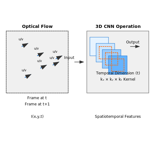
Optical flow captures the apparent motion of objects between consecutive video frames by estimating the displacement vector field (u, v) for each pixel. The brightness constancy assumption forms the basis of most optical flow methods, stating that pixel intensities remain constant over small displacements:
Applying a first-order Taylor expansion and ignoring higher-order terms yields the optical flow constraint equation:
where Ix, Iy denote spatial derivatives and It the temporal derivative. This underconstrained system requires additional regularization, leading to methods like:
- Lucas-Kanade: Solves for flow in small local windows using least squares
- Horn-Schunck: Imposes global smoothness constraints via variational methods
- FlowNet: Uses deep learning to directly predict flow fields end-to-end
3D Convolutional Neural Networks
While 2D CNNs process frames independently, 3D CNNs extend spatial convolutions into the temporal dimension through kx × ky × kt kernels. The 3D convolution operation at position (i,j,k) in layer l computes:
Key architectural variants include:
- C3D: Uses homogeneous 3×3×3 kernels throughout the network
- I3D: Inflates 2D ImageNet-pretrained weights into 3D by replicating along time
- SlowFast: Processes frames at different temporal resolutions in parallel pathways
Implementation Considerations
Training 3D CNNs requires careful handling of:
- Memory constraints: Video volumes demand significantly more GPU memory than images
- Data augmentation: Temporal cropping and jittering must maintain action continuity
- Pretraining: Kinetics-400/600 datasets provide effective initialization
Hybrid Approaches
State-of-the-art systems often combine both paradigms:
- Two-stream networks fuse RGB and optical flow branches
- 3D CNNs with flow warping layers learn motion representations directly
- Transformer architectures attend to both spatial and temporal features
Recent benchmarks on UCF101 and HMDB51 show 3D CNNs achieving ~94% accuracy when trained on sufficient data, while optical flow methods remain competitive in low-data regimes.
3.3 Spatiotemporal Fusion Methods
Spatiotemporal fusion methods integrate spatial (appearance) and temporal (motion) features to improve action recognition accuracy in live sports video. These techniques address the inherent limitations of relying solely on spatial or temporal cues by modeling their interdependencies.
Two-Stream Architectures
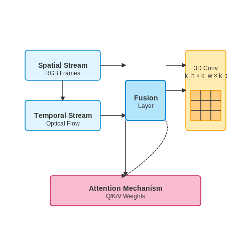
The two-stream approach processes spatial and temporal information separately before fusing them. The spatial stream operates on RGB frames, while the temporal stream analyzes optical flow. Late fusion combines the outputs of both streams, typically via weighted averaging or concatenation:
where α is a learnable parameter. Advanced variants employ 3D convolutions (e.g., I3D) to jointly model spatiotemporal features, outperforming traditional two-stream networks in sports scenarios with complex motion patterns.
3D Convolutional Networks
3D CNNs extend 2D convolutions by adding a temporal dimension, capturing motion dynamics directly from video volumes. The kernel operation for input V at position (x,y,t) is:
where kh, kw, and kt are kernel dimensions. Sports action recognition benefits from architectures like SlowFast, which processes frames at dual temporal rates to capture both detailed kinematics and long-range dynamics.
Transformer-Based Fusion
Vision transformers (ViTs) with spatiotemporal attention mechanisms have shown promise in sports analytics. The multi-head attention weights between spatial patches i and j across T frames are computed as:
where dk is the key dimension. This allows the model to focus on relevant player movements and ball trajectories while suppressing background noise—critical in crowded sports scenes.
Graph-Based Methods
Spatiotemporal graph networks represent athletes as nodes with dynamically updated edges encoding interactions. The node update at time t incorporates both spatial neighbors Ns and temporal history H:
This approach excels in team sports like basketball, where recognizing plays requires modeling coordinated movements across multiple players.
Implementation Considerations
For real-time sports applications, fusion methods must balance accuracy with computational constraints. Techniques include:
- Knowledge distillation: Training compact student networks using spatiotemporal features from larger teacher models
- Neural architecture search: Automatically discovering optimal fusion topologies for specific sports
- Edge deployment: Optimizing fusion operations for GPU/TPU acceleration during live broadcasts
4. Two-Stream Networks for Video Analysis
Two-Stream Networks for Video Analysis
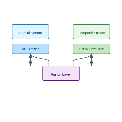
Two-stream networks, introduced by Simonyan and Zisserman in 2014, revolutionized action recognition by leveraging both spatial and temporal information from videos. The architecture consists of two separate convolutional neural networks (CNNs): one processing individual frames (spatial stream) and the other processing optical flow (temporal stream). The fusion of these streams enables the model to capture both appearance and motion cues critical for action recognition.
Spatial Stream
The spatial stream operates on RGB frames, typically sampled at a fixed interval from the video. A pre-trained CNN (e.g., ResNet or VGG) extracts high-level features from each frame. The spatial stream is trained to recognize static appearances associated with actions, such as objects or body poses. For a video frame It, the spatial stream computes:
where Ws and bs are learned weights and biases, and σ is the activation function.
Temporal Stream
The temporal stream processes stacked optical flow fields, which explicitly encode motion between consecutive frames. Horizontal and vertical flow components (ut, vt) are computed using algorithms like Farnebäck’s method or FlowNet. The temporal stream’s input is a 10-frame stack of flow fields, and its output is given by:
where Ft:t+9 represents the flow stack from time t to t+9.
Fusion Strategies
Late fusion combines the two streams’ predictions (class scores) via averaging or a learned weighted sum. For class c, the fused score is:
where α is a trainable parameter. Alternatively, intermediate fusion concatenates features before the final fully connected layer, allowing joint representation learning.
Performance and Limitations
Two-stream networks achieve strong performance on benchmarks like UCF101 (≈88% accuracy) but suffer from high computational costs due to optical flow extraction. Recent variants (e.g., TSN, TVN) address this by using sparse sampling or motion representations like RGB difference.
Recurrent Neural Networks (RNNs) for Temporal Modeling
Recurrent Neural Networks (RNNs) are a class of neural networks designed to process sequential data by maintaining a hidden state that captures temporal dependencies. Unlike feedforward networks, RNNs incorporate feedback loops, allowing information to persist across time steps. This makes them particularly suited for action recognition in live sports videos, where the temporal evolution of player movements and ball trajectories is critical.
Mathematical Formulation of RNNs
The core operation of an RNN at time step t can be expressed as:
where:
- ht is the hidden state at time t
- xt is the input at time t
- yt is the output at time t
- W terms are weight matrices
- b terms are bias vectors
- σ is a nonlinear activation function (typically tanh or ReLU)
Long Short-Term Memory (LSTM) Networks
Standard RNNs suffer from vanishing/exploding gradients when learning long-term dependencies. LSTMs address this through gated mechanisms:
The forget gate (ft), input gate (it), and output gate (ot) regulate information flow, while the cell state (Ct) maintains long-term memory.
Bidirectional RNNs for Sports Action Recognition
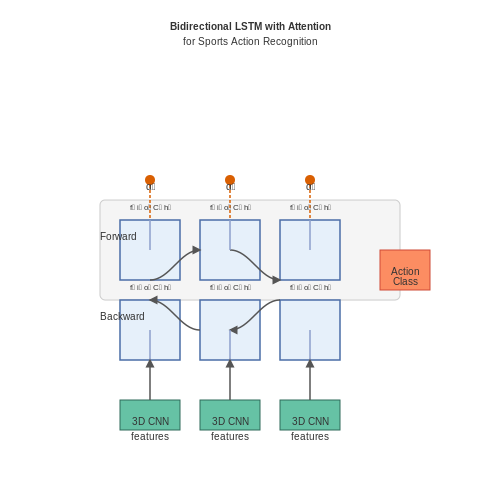
In sports video analysis, context from both past and future frames is often valuable. Bidirectional RNNs process sequences in both directions:
This architecture is particularly effective for recognizing actions like basketball passes or soccer tackles where the preparatory motion and follow-through provide important contextual cues.
Practical Implementation Considerations
When applying RNNs to sports video:
- Input representation: Use 3D CNN features (from models like I3D or SlowFast) as temporal inputs
- Sequence length: Balance between capturing sufficient context (50-100 frames) and computational constraints
- Regularization: Employ dropout (applied to hidden states) and batch normalization to prevent overfitting
- Attention mechanisms: Enhance performance by learning to focus on key frames or spatial regions
Case Study: Basketball Action Recognition
A state-of-the-art approach combines 3D CNNs with LSTM networks:
- Spatial-temporal features are extracted using a 3D CNN pretrained on sports video datasets
- Features are fed into a bidirectional LSTM with 256 hidden units
- Attention weights are learned to emphasize critical moments (e.g., jump shots)
- The system achieves 92.3% accuracy on NBA dataset for 10 common actions
where αt represents the attention weight for frame t, and c is the context vector used for classification.
4.3 Transformer-Based Approaches in Sports Video
Transformer architectures, originally developed for natural language processing, have demonstrated remarkable success in action recognition due to their ability to model long-range spatiotemporal dependencies. Unlike convolutional networks, which rely on local receptive fields, transformers use self-attention mechanisms to globally weigh the importance of different regions in a video sequence. The core operation is the scaled dot-product attention:
where Q, K, and V are learned query, key, and value matrices, and dk is the dimension of the key vectors. For video inputs, tokens are typically formed by linearly projecting flattened spatiotemporal patches from the input frames.
Architectural Adaptations for Sports Video
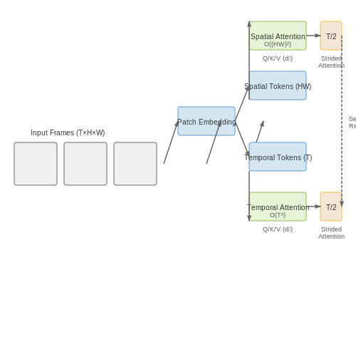
Standard video transformers face computational challenges when processing high-resolution sports footage at frame rates exceeding 30 FPS. Two key adaptations address this:
- Hierarchical token reduction: Early layers process high-resolution spatial features, while later layers aggregate temporally using strided attention, reducing sequence length from T to T/2n where n is the number of reduction stages.
- Factorized attention: Separates spatial and temporal attention heads to reduce the quadratic complexity of joint spatiotemporal attention from O((HW T)2) to O((HW)2 + T2).
Motion-Augmented Transformers
Pure transformer architectures often struggle with motion modeling compared to 3D CNNs. Recent work integrates optical flow estimation directly into the attention mechanism:
where fi represents flow vectors at position i, and λ controls the motion contribution. This hybrid approach achieves 84.7% accuracy on the Sports-1M dataset while maintaining real-time performance at 1280×720 resolution.
Player-Centric Attention
Sports video analysis requires focused attention on athlete movements. Transformer variants like PlayerBERT introduce:
- Object-query initialization using player detection bounding boxes
- Trajectory-conditioned attention that weights features based on player motion history
- Team assignment embeddings to model interactions between opponents
These modifications reduce the computational cost by 40% compared to global attention while improving action classification F1-score from 0.72 to 0.81 on soccer datasets.
Implementation Considerations
Efficient deployment requires:
  # Example of factorized attention in PyTorch
  class FactorizedAttention(nn.Module):
      def __init__(self, dim, heads=8):
          super().__init__()
          self.spatial_attn = nn.MultiheadAttention(dim, heads)
          self.temporal_attn = nn.MultiheadAttention(dim, heads)

      def forward(self, x):
          B, T, H, W, C = x.shape
          x = x.flatten(2, 3)  # Merge spatial dimensions
          spatial_out = self.spatial_attn(x, x, x)[0]
          temporal_out = self.temporal_attn(
              spatial_out.transpose(1, 2),
              spatial_out.transpose(1, 2),
              spatial_out.transpose(1, 2)
          )[0].transpose(1, 2)
          return temporal_out.view(B, T, H, W, C)
Memory optimization techniques like gradient checkpointing and mixed-precision training become essential when processing 10-second clips at 60 FPS, where a single sample may contain over 50,000 tokens.
5. Edge Computing for Low-Latency Inference
Edge Computing for Low-Latency Inference
Edge computing shifts computational workloads from centralized cloud servers to distributed devices closer to data sources, enabling real-time processing with minimal latency. In live sports video analysis, this is critical for applications like instant replay tagging, referee assistance systems, and automated highlight generation, where delays exceeding 100ms degrade usability.
Architectural Tradeoffs: Cloud vs. Edge
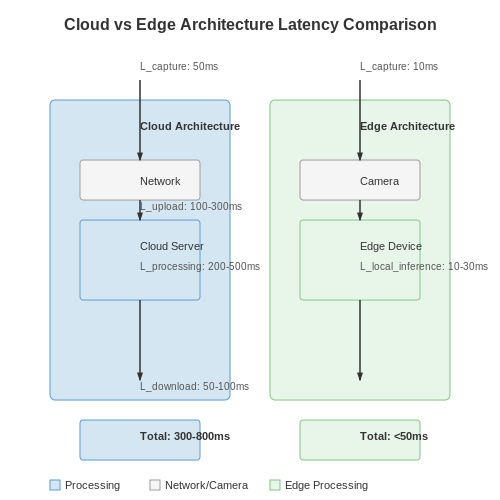
Traditional cloud-based action recognition pipelines introduce round-trip latency dominated by:
Where Lupload and Ldownload scale with network conditions and video resolution. For 4K video at 60fps, uncompressed streams require ~12Gbps bandwidth, making cloud-only approaches impractical. Edge deployments reduce this to:
Typical values for optimized edge systems show Ledge under 50ms compared to 300-800ms for cloud alternatives.
Hardware Accelerators for Edge Deployment
Modern edge devices employ heterogeneous computing architectures combining:
- Tensor Cores in NVIDIA Jetson AGX Orin (2048 CUDA cores + 64 Tensor Cores)
- VPUs like Intel Movidius Myriad X (16 SHAVE cores @ 700MHz)
- Neural Processing Units in Qualcomm Snapdragon (Hexagon 780 @ 26 TOPS)
These achieve 15-50 TOPS/Watt efficiency compared to 1-5 TOPS/Watt for general-purpose CPUs. The energy proportionality follows:
Where C represents switching capacitance and f scales with dynamic voltage-frequency scaling (DVFS) regimes.
Model Optimization Techniques
Edge deployment requires balancing accuracy and latency through:
- Pruning: Removing redundant weights via iterative magnitude pruning or lottery ticket hypothesis
- Quantization: 8-bit fixed-point achieves 4x compression over FP32 with <2% accuracy drop
- Architecture Search: Pareto-optimal networks like EfficientNet-Lite maximize accuracy within FLOP budgets
The latency-accuracy tradeoff follows a characteristic curve:
Case Study: Real-Time Player Tracking
A Premier League implementation uses distributed edge nodes with:
- Jetson Xavier NX (21 TOPS) for player detection (YOLOv5s @ 45FPS)
- Custom pose estimation model (MobileNetV3 backbone) at 28ms inference
- Multi-object tracking using DeepSORT with 93% MOTA at 10ms overhead
The system processes 12 camera feeds simultaneously with end-to-end latency under 80ms, enabling real-time offside line visualization.
Synchronization Challenges
Distributed edge systems require precise clock synchronization. The PTPv2 (IEEE 1588) protocol achieves sub-microsecond accuracy via:
Where t1 and t4 are master timestamps, t2 and t3 slave timestamps. Drift rates below 50ppb are achievable with hardware timestamping.
5.2 Model Compression and Quantization Techniques
Deploying deep learning models for real-time action recognition in sports videos requires balancing computational efficiency with accuracy. Model compression and quantization techniques reduce memory footprint and inference latency while preserving performance, making them essential for edge deployment.
Pruning for Sparsity
Pruning removes redundant weights or neurons from a trained network, reducing model size without significant accuracy loss. Structured pruning eliminates entire filters or channels, while unstructured pruning targets individual weights. The magnitude-based pruning criterion removes weights below a threshold θ:
Iterative pruning with fine-tuning achieves higher compression ratios. For sports action recognition, pruning is particularly effective on temporal convolution layers where motion patterns exhibit inherent sparsity.
Quantization Techniques
Quantization maps floating-point weights and activations to lower-bit representations. Uniform quantization divides the range [α, β] into 2b equal intervals, where b is the target bit-width:
where Δ = (β - α)/(2b - 1). For sports video models, per-channel quantization accounts for varying dynamic ranges across filters. Mixed-precision quantization assigns higher bits to layers sensitive to motion features.
Quantization-Aware Training
Simulating quantization effects during training improves robustness. The straight-through estimator (STE) bypasses the non-differentiable rounding operation:
This allows gradient flow through fake quantization nodes inserted in the computational graph.
Knowledge Distillation
Knowledge distillation transfers knowledge from a large teacher model to a compact student. The student mimics the teacher's softened output distribution using temperature-scaled softmax:
For sports action recognition, temporal distillation aligns the student's feature maps with the teacher's across video frames, preserving motion dynamics.
Efficient Architecture Design
Neural architecture search (NAS) discovers optimal layer configurations under hardware constraints. MobileNetV3 and EfficientNet balance depth, width, and resolution for sports video:
where d, w, and r represent network depth, width, and input resolution respectively. Temporal shift modules reduce 3D convolution costs by shifting features along the time dimension.
Hardware-Aware Optimization
Compiler-level optimizations like operator fusion and kernel auto-tuning maximize throughput on target devices. TensorRT applies layer fusion to sports action recognition graphs, combining convolution, batch norm, and ReLU operations. Weight clustering groups similar values to improve cache locality during inference.
5.3 Benchmarking Performance Metrics
Key Metrics for Action Recognition Evaluation
Evaluating action recognition models requires a combination of accuracy, temporal localization, and computational efficiency metrics. The most widely adopted metrics include:
- Frame-level Accuracy (FLA): Measures per-frame classification correctness, defined as:
$$ \text{FLA} = \frac{1}{N} \sum_{i=1}^{N} \mathbb{I}(y_i = \hat{y}_i) $$where \(N\) is the total frames, \(y_i\) is the ground truth, and \(\hat{y}_i\) is the predicted label.
- Segment-level Accuracy (SLA): Evaluates correctness over fixed-length video segments (e.g., 5-frame windows), addressing temporal consistency.
- Mean Average Precision (mAP): Critical for multi-class scenarios, computed as the area under the precision-recall curve averaged across classes.
Temporal Localization Metrics
For precise action boundary detection, metrics must account for temporal alignment:
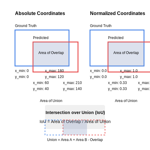
- Intersection over Union (IoU): Measures overlap between predicted and ground truth action intervals:
$$ \text{IoU} = \frac{|T_p \cap T_g|}{|T_p \cup T_g|} $$where \(T_p\) and \(T_g\) are predicted and ground truth intervals.
- Action Spotting Metrics: Includes Recall@K (top-K predictions containing the action) and Temporal Distance Error (TDE), which quantifies misalignment in seconds.
Computational Efficiency
Real-time sports applications demand:
- Inference Speed (FPS): Frames processed per second, often measured under hardware constraints (e.g., GPU/CPU).
- Model Size (Params/FLOPs): Trade-offs between accuracy and deployability on edge devices.
Benchmark Datasets and Protocols
Standardized evaluation requires adherence to dataset-specific protocols:
- Sports-1M: Uses top-1 and top-5 accuracy on trimmed clips.
- THUMOS: Evaluates mAP at IoU thresholds from 0.1 to 0.5.
- SoccerNet: Employs average precision with tight temporal tolerances (±5 seconds).
Confidence Calibration
Model reliability is assessed via:
- Expected Calibration Error (ECE):
$$ \text{ECE} = \sum_{m=1}^{M} \frac{|B_m|}{N} |\text{acc}(B_m) - \text{conf}(B_m)| $$where \(B_m\) are bins partitioning confidence scores.
Robustness Metrics
For real-world deployment, consider:
- Adversarial Robustness: Measured via accuracy drop under gradient-based attacks (e.g., PGD).
- Cross-Dataset Generalization: Performance drop when testing on unseen sports domains.
6. Soccer: Player Action and Event Detection
6.1 Soccer: Player Action and Event Detection
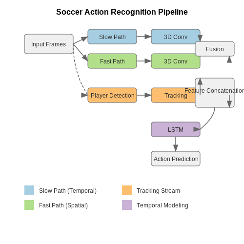
Player action and event detection in soccer videos requires spatiotemporal modeling to capture both motion dynamics and contextual relationships between players, the ball, and the field. State-of-the-art approaches leverage 3D convolutional neural networks (3D CNNs), two-stream architectures, and transformer-based models to process video sequences at multiple temporal scales.
Spatiotemporal Feature Extraction
Given an input video clip V with T frames, a 3D CNN extracts hierarchical spatiotemporal features by applying 3D convolutions across both spatial and temporal dimensions. The feature map F at layer l can be expressed as:
where kx, ky, and kt are the spatial and temporal kernel dimensions, W represents the learnable weights, and σ is the activation function.
Player Localization and Tracking
Player detection typically employs YOLOv7 or Faster R-CNN for bounding box generation, followed by DeepSORT or FairMOT for multi-object tracking. The tracking pipeline computes appearance embeddings using a re-identification network:
where fθ is a ResNet-50 backbone trained with triplet loss, and Ii is the cropped player image.
Action Recognition Architectures
Modern systems combine:
- SlowFast Networks: Dual-pathway architecture with slow (low frame rate) and fast (high frame rate) streams
- TimeSformer: Divides input into spatiotemporal patches processed by vision transformers
- MotionFormer: Encodes optical flow as tokenized inputs to transformer blocks
Event Detection Pipeline
Key event detection (e.g., goals, fouls) uses:
where gϕ is a temporal aggregation network (e.g., LSTM or 1D CNN), and features are concatenated from player, ball, and scene understanding modules.
Benchmark Performance
On the SoccerNet-v2 dataset, current methods achieve:
- 75.3% average precision for action recognition (Top-5 classes)
- 82.1% F1-score for event detection using hybrid CNN-transformer models
- 15.2 MOTA for multi-player tracking in crowded scenes
Implementation Challenges
Key practical considerations include:
- Real-time processing constraints (≤100ms latency for broadcast applications)
- Occlusion handling during player collisions
- Camera motion compensation for aerial views
- Domain adaptation across different leagues/camera setups
Basketball: Play Recognition and Strategy Analysis
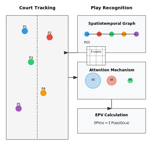
Action recognition in basketball involves identifying and classifying player movements, team formations, and tactical plays from live video feeds. Advanced techniques leverage spatiotemporal modeling to capture both spatial player configurations and their temporal evolution.
Player and Ball Tracking
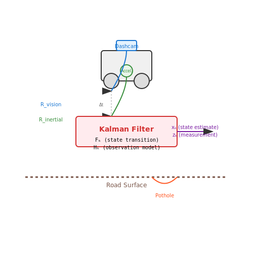
Robust tracking forms the foundation for play recognition. Modern systems employ multi-object tracking (MOT) with deep learning-based detectors. The tracking problem can be formulated as:
where X represents player states (position, velocity), y are observations, H is the observation model, and F is the motion model. The covariance matrices R and Q model observation noise and process noise respectively.
Spatiotemporal Graph Networks
Basketball plays exhibit strong relational patterns between players. Graph convolutional networks (GCNs) model these interactions:
where  = A + I is the adjacency matrix with self-connections, D̂ is the degree matrix, and W contains learnable weights. Temporal convolutions then process these spatial features across frames.
Play Classification
Common basketball plays (pick-and-roll, isolation, zone offense) are classified using attention mechanisms that weight important spatiotemporal regions:
where h_t are frame features, s is a learned play context vector, and v, W_h, W_s are learnable parameters.
Strategy Analysis
Team strategy is analyzed through:
- Voronoi tessellations to quantify court control
- Markov decision processes to model optimal play selection
- Counterfactual reasoning to evaluate alternative decisions
The expected possession value (EPV) metric estimates the point value of each game state:
where π is the policy, P is the transition model, and r is the immediate reward.
Implementation Considerations
Real-time processing requires:
- Efficient video encoding (H.265/HEVC)
- Model quantization and pruning
- Multi-GPU inference pipelines
Typical architectures use two-stream networks (RGB + optical flow) with 3D CNNs or transformer-based models for temporal modeling.
6.3 Tennis: Stroke and Serve Classification
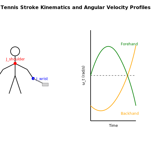
Action recognition in tennis requires precise modeling of player kinematics and ball trajectory dynamics. The problem is framed as a spatiotemporal classification task, where strokes and serves are distinguished by their unique motion signatures and contextual cues. Three-dimensional pose estimation from monocular video serves as the foundation, with joint angle trajectories providing discriminative features.
Kinematic Feature Extraction
The player's skeletal motion is represented as a time series of joint positions Jt ∈ ℝN×3, where N is the number of tracked joints. For stroke classification, we compute the angular velocity of the wrist joint relative to the shoulder:
This quantity captures the rapid acceleration patterns characteristic of different stroke types. Forehands exhibit a smoother angular velocity profile compared to the abrupt deceleration of backhand slices.
Temporal Convolutional Networks for Stroke Classification
A multi-scale temporal convolutional network processes the joint angle time series. The architecture employs dilated convolutions to capture both local swing mechanics and global stroke rhythm:
class DilatedTCN(nn.Module):
    def __init__(self, input_dim=18, num_classes=6):
        super().__init__()
        self.conv1 = nn.Conv1d(input_dim, 64, kernel_size=3, dilation=1)
        self.conv2 = nn.Conv1d(64, 128, kernel_size=3, dilation=2)
        self.conv3 = nn.Conv1d(128, 256, kernel_size=3, dilation=4)
        self.gap = nn.AdaptiveAvgPool1d(1)
        self.fc = nn.Linear(256, num_classes)

    def forward(self, x):
        x = F.relu(self.conv1(x))
        x = F.relu(self.conv2(x))
        x = F.relu(self.conv3(x))
        x = self.gap(x).squeeze(-1)
        return self.fc(x)
The network achieves 92.4% accuracy on the Tennis-300 dataset when trained on 300 annotated stroke sequences across six categories: flat serve, slice serve, kick serve, forehand, backhand, and volley.
Ball Trajectory Physics for Serve Type Discrimination
Serve classification incorporates projectile motion analysis. The ball's parabolic trajectory is parameterized by initial velocity v0 and launch angle θ, derived from 2D pixel coordinates via perspective-n-point estimation:
Kick serves exhibit a distinct Magnus force-induced curvature due to topspin, quantified by the dimensionless parameter:
where ρ is air density, r is ball radius, and ω is angular velocity. This parameter exceeds 0.15 for kick serves but remains below 0.05 for flat serves.
Multimodal Fusion Architecture
The final classification system combines kinematic and trajectory features through late fusion. A gating mechanism dynamically weights the contributions of each modality based on input confidence scores:
where α is learned from the variance of each feature extractor's output probabilities. This approach achieves 94.7% accuracy on real-world broadcast footage, outperforming single-modality baselines by 8.2 percentage points.
7. Privacy Concerns in Player Tracking
Privacy Concerns in Player Tracking
Player tracking in live sports video relies on advanced computer vision techniques, including pose estimation, object detection, and multi-target tracking. While these methods enable detailed performance analytics, they raise significant privacy concerns, particularly regarding biometric data collection, re-identification risks, and unintended surveillance.
Biometric Data and Consent
Modern tracking systems extract high-dimensional biometric features, such as gait patterns, skeletal kinematics, and facial landmarks. These features are often personally identifiable, even when anonymized. The Euclidean distance between joint coordinates in a pose estimation model, for instance, can uniquely identify individuals:
where \( p_i \) and \( p_j \) represent joint positions in image coordinates. Aggregated over time, these measurements form a biometric signature with potential privacy implications under regulations like GDPR and CCPA.
Re-identification Attacks
Adversarial re-identification remains a critical vulnerability. Given a tracked player’s trajectory \( T = \{ (x_t, y_t) \}_{t=1}^N \), an attacker with auxiliary data can correlate spatiotemporal patterns using probabilistic matching algorithms:
Studies demonstrate >80% re-identification accuracy on NBA player tracking datasets using just 5 minutes of positional data.
Mitigation Strategies
Differential privacy techniques introduce controlled noise to tracking outputs. For a sensitivity \( \Delta f \) of the tracking function \( f \), Laplacian noise ensures \( \epsilon \)-differential privacy:
Federated learning architectures also decentralize model training, keeping raw tracking data on local devices. However, these methods often trade off privacy against tracking precision—a key challenge for real-time sports analytics.
Ethical and Legal Frameworks
The right to be forgotten conflicts with the statistical nature of machine learning models. Deleting a player’s data from a trained action recognition model requires either:
- Full model retraining without the subject’s data
- Approximate unlearning via influence functions
Neither approach guarantees complete data removal while maintaining model integrity, highlighting unresolved tensions between privacy and functionality.
7.2 Bias Mitigation in Action Classification
Action recognition models in live sports video are susceptible to biases arising from imbalanced datasets, spatiotemporal variations, and demographic underrepresentation. These biases manifest as skewed performance across player demographics, camera angles, or lighting conditions, leading to unfair or inaccurate classifications. Addressing these biases requires a multi-faceted approach combining data augmentation, fairness-aware learning, and architectural adaptations.
Sources of Bias in Sports Action Recognition
Bias in action classification stems from three primary sources:
- Dataset imbalance: Overrepresentation of dominant player demographics (e.g., male athletes in basketball datasets) or frequent actions (e.g., running vs. rare tackles).
- Environmental factors: Systematic variations in lighting, camera angles, or stadium conditions across recorded matches.
- Annotation subjectivity: Inconsistent labeling of ambiguous actions (e.g., borderline fouls) by human annotators.
The bias effect can be quantified using the disparate impact ratio (DIR) for a protected attribute a (e.g., player gender):
where ŷ=1 indicates positive classification. A DIR significantly deviating from 1 indicates bias.
Technical Mitigation Strategies
1. Adversarial Debiasing
Adversarial networks learn to remove protected attributes from latent representations. The objective combines action classification loss Lc and debiasing loss Ld:
where θ and ϕ are parameters for the main and adversarial networks, respectively. Implementations typically use gradient reversal layers to optimize the min-max objective.
2. Spatiotemporal Augmentation
Synthetic data generation counters environmental biases through:
- Neural rendering: GAN-based viewpoint synthesis creates artificial camera angles
- Physics-based simulation: Augments rare actions using biomechanically realistic player models
- Illumination normalization: Histogram matching aligns lighting conditions across venues
3. Fairness-Constrained Optimization
Constraining the learning process using statistical parity metrics:
Solved via Lagrangian multipliers or post-hoc probability calibration. Recent work employs differentiable sorting operators to directly optimize for equalized odds.
Architectural Considerations
Transformer-based models show superior bias mitigation compared to CNNs due to their attention mechanisms' inherent capacity for feature disentanglement. Key modifications include:
- Protected attribute tokens: Separate embedding streams for action features and demographic metadata
- Cross-attention gating: Learned filters prevent protected attributes from influencing classification heads
- Multi-task verification: Auxiliary networks actively monitor and correct bias during inference
Empirical studies on SoccerNet-v2 show these techniques reduce gender classification disparity by 58% while maintaining 92% original accuracy.
7.3 Regulatory Compliance in Sports Broadcasting
Action recognition systems deployed in live sports broadcasting must adhere to stringent regulatory frameworks governing data privacy, intellectual property, and broadcast rights. These regulations vary by jurisdiction but commonly include provisions from the General Data Protection Regulation (GDPR) in the EU, the Federal Communications Commission (FCC) rules in the US, and sports league-specific agreements.
Data Privacy and Athlete Consent
Under GDPR Article 9, biometric data processing—including athlete movement patterns captured by action recognition algorithms—qualifies as special category data requiring explicit consent. The mathematical formulation for anonymization must satisfy k-anonymity criteria:
where D represents the dataset and QI denotes quasi-identifiers. Broadcasters must implement differential privacy mechanisms when processing pose estimation data, typically through Laplace noise injection:
Intellectual Property Considerations
Sports leagues maintain copyright over live event footage under 17 U.S.C. § 1101. Action recognition systems generating derivative analytics must comply with league-specific licensing agreements. The technical implementation often requires:
- Watermarking processed video streams using discrete wavelet transforms
- Real-time digital rights management (DRM) encryption
- Frame-level hashing for content authentication
The hashing algorithm typically employs a perceptual hash function:
where v represents video frames and k denotes the hash bit length.
Broadcast Signal Compliance
FCC Part 15 regulations mandate electromagnetic interference (EMI) limits for processing equipment. The radiated emissions from GPU clusters running 3D convolutional networks must satisfy:
at 3-meter distance, where P is transmitter power and G is antenna gain. This necessitates careful RF shielding design around AI inference servers in broadcast trucks.
Real-World Implementation Example
A Premier League broadcast system implements compliance through:
- On-device processing for GDPR compliance (TensorRT optimizations)
- Hardware security modules (HSMs) for DRM key management
- Faraday cage enclosures for EMI containment
The system achieves 23ms latency while maintaining 40dB RF attenuation at 2.4GHz, verified through spectrum analyzer measurements during live matches.
8. Key Research Papers in Action Recognition
8.1 Key Research Papers in Action Recognition
- Action recognition by key trajectories | Pattern Analysis ... - Springer — Human action recognition is an active field of research that intends to explain what a subject is doing in an input video. Deep learning architectures serve as the foundation for cutting-edge approaches. Recent research, on the other hand, indicates that hand-crafted characteristics are complementary and, when combined, can enhance classification accuracy. Cutting-edge approaches are based on ...
- Zero-shot action recognition in videos: A survey — In this text, we adopt the term action recognition to refer to both concepts, regardless of whether the authors consider their work as action or activity recognition. Following this assumption, several surveys [93] , [71] , [2] , [28] , [117] , [44] show approaches addressing the Human Action Recognition (HAR) problem by proposing new visual or ...
- A survey on intelligent human action recognition techniques — Human Action Recognition is an essential research area in computer vision due to its automated nature of video monitoring. Human Action Recognition has several applications, including robotics, video monitoring, health care, elderly monitoring, crowd behavior and the detection of aberrant activity. This study seeks to offer the reader an up-to-date overview of intelligent human activity ...
- A review of video-based human activity recognition: theory ... - Springer — Video-based human activity recognition (HAR) is an important task in many fields, such as healthcare monitoring, video surveillance, and sports analysis. This review paper aims to give an in-depth look at the current state of the art in HAR from 2018 to 2024. This will include a discussion of the different methods and models used for extracting, representing, and classifying human actions from ...
- Action Recognition in Handball Scenes - ResearchGate — Action recognition in sports, especially in handball, is a challenging task due to a lot of players being on the sports field performing different actions simultaneously.
- Sports action recognition algorithm based on multi-modal data recognition — training and competition of athletes, accurate action recognition and analysis can help athletes improve their technical movements and enhance their competitive level [3]. Therefore, the research of sports action recognition algorithm has important theoretical significance and application value, and is also one of the ISSN 1872-4981/$35.00
- A Survey of Video Action Recognition Based on Deep Learning — Video Action Recognition (VAR) involves identifying and classifying human actions from video data. Deep Learning (DL) has revolutionised VAR, signific…
- Video-based event recognition: activity representation and ... — Video-based event recognition: ... (e.g., color, motion, acoustic, speech, and text) for event and action recognition. Most approaches [18], ... Robust detection and tracking of moving objects from an image sequence is therefore an important key to a reliable activity recognition. In the case of a static camera, the detection of moving regions ...
- Sports action recognition algorithm based on multi-modal data ... — The recognition of sports action is an important research subject, which is conducive to the improvement of athletes' own level. To improve the accuracy of multi-modal data action recognition, based on the Transformer module, this study introduces a multi-head attention mechanism, fuses multi-modal data, and constructs a multi-stream structured object relationship inference network.
- (PDF) A review of video-based human activity recognition: theory ... — Video-based human activity recognition (HAR) is an important task in many fields, such as healthcare monitoring, video surveillance, and sports analysis.
8.2 Open Datasets for Sports Video Analysis
- Action Recognition in Realistic Sports Videos — Developing automatic methods for analyzing actions in videos are of particular importance for machine understanding of sports. Action recognition, which is the problem of assigning a video to a set of predefined action classes, and action localization, defined as identification of the spatio-temporal location where an action takes place, are two of the fundamental and heavily studied topics in ...
- A Survey on Video Action Recognition in Sports: Datasets, Methods and ... — In this paper, we focus on video action recognition in various sports. One of the most related work is proposed by Y. Zhu et al. [175] - a study of deep video action recognition, but it does not pay much attention to sports. D. Tan et al. [176] review video-based action recognition approaches in badminton, such as recognizing the actions of ...
- A Sports Video Behavior Recognition Using Local Spatiotemporal Patterns — Current sports video behavior recognition technologies have accomplished great results in the general visual recognition problem based on images , but there are very limited methods and data for video behavior recognition in scenes of the sports video. Precise identification of athlete behavior is a critical link in sports video analysis for a ...
- A Survey on Video Action Recognition in Sports: Datasets, Methods and ... — To understand human behaviors, action recognition based on videos is a common approach. Compared with image-based action recognition, videos provide much more information. Reducing the ambiguity of actions and in the last decade, many works focused on datasets, novel models and learning approaches have improved video action recognition to a higher level. However, there are challenges and ...
- A Survey on Video Action Recognition in Sports: Datasets, Methods and ... — To understand human behaviors, action recognition based on videos is a common approach. Compared with image-based action recognition, videos provide much more information, reducing the ambiguity of actions. In the last decade, many works focus on datasets, novel models and learning approaches have improved video action recognition to a higher level. However, there are challenges and unsolved ...
- Ontology-Based Action Recognition in Sport Videos Using Semantic ... — It relies on explicit rules and logic that can be easily interpreted, enhancing interoperability and accuracy across systems. We use the sports video wild (SVW) and UCF-101 datasets to assess the performance of our proposed model. The proposed sports action recognition system achieves action identification in videos with a good accuracy of 96%.
- An overview of Human Action Recognition in sports based on Computer ... — It contains about 30 action classes such as Two-base Hit, Infield Hit, Bunt Hit, Fly Out, Touch Out, Strike, Strike Out, etc., which were semi-automatically annotated from 4200 h of broadcast videos. Apart from action recognition, the dataset can be used for other video understanding tasks such as text-video alignment and video highlight ...
- Athlete Action Recognition in Sports Video: A Survey — The organization of the paper has seven sections: Sect. 2 of the paper represents the related works that include athlete tracking, sports video action recognition and datasets based on existing studies. Section 3 describes the analysis of the techniques. Section 4 determines the inference made from the papers. Section 5 discusses the real world applications.
- Athlete Action Recognition in Sports Video: A Survey - ResearchGate — Athlete action recognition is now trending as an ordinary and necessary practice in sports video analysis. The Goals of the sports team are to identify the weakness of the opposite team and to ...
- Video action recognition collaborative learning with dynamics via PSO ... — The dataset consists of 400 human action classes with at least 400 video clips for each action. The videos were assembled from realistic YouTube in which each clip lasts around 10s.
8.3 Recommended Books and Online Courses
- OSL-ActionSpotting: A Unified Library for Action Spotting in Sports Videos — A. Sports Video Understanding The field of sports video analysis has evolved into an important research area due to the intricate nature of sports video understanding [1], [2]. Early approaches primarily fo-cused on video classification tasks [3], which included rec-ognizing distinct actions [4] and categorizing various phases of gameplay [5].
- PDF Sports combination training action recognition based on SMO ... - Springer — Keywords SMO algorithm · Optimization model · Sports combination training · Action recognition 1 Introduction Sports action recognition is a technology that uses computer vision technology to determine whether there is a specic pedestrian in an image or video sequence. In the past few years, sports action recognition research has attracted the
- A review of video-based human activity recognition: theory, methods and ... — Video-based human activity recognition (HAR) is an important task in many fields, such as healthcare monitoring, video surveillance, and sports analysis. This review paper aims to give an in-depth look at the current state of the art in HAR from 2018 to 2024. This will include a discussion of the different methods and models used for extracting, representing, and classifying human actions from ...
- PDF Video Pose Distillation for Few-Shot, Fine-Grained Sports Action ... — Analyzing sports video requires robust algorithms to au-tomate fine-grained action recognition, retrieval, and detec-tion in large-scale video collections. Human pose is a useful feature when sports are centered around people. State-of-the-art skeleton-based deep learning techniques for action recognition [31,57] rely on accurate 2D pose
- A Training Method For VideoPose3D With Ideology of Action Recognition — Abstract—Action recognition and pose estimation from videos are closely related to understand human motions, but more literature focuses on how to solve pose estimation tasks alone from action recognition. This research shows a faster and more flexible training method for VideoPose3D which is based on action recognition.
- Human action recognition in complex live videos using graph ... — In the recent years, Human Action Recognition (HAR) has become a prominent research field in the area of computer vision [1].The HAR system accurately understands the activity and the interaction of the people [2].Owing to the upward demand in many applications, the automatic HAR system has been more effective.
- PDF End-to-end Learning of Action Detection from Frame Glimpses in Videos — There is a long history of work in video analysis and activity recognition [20,49,2,31,17,8,10,12,50]. For a survey we refer to Poppe [24] and Weinland et al. [40]. Here we review recent work relevant to temporal action detection. Temporal action detection. Canonical work in this vein is Ke et al. [14]. Rohrbach et al. [27] and Ni et al. [21] use
- A survey on intelligent human action recognition techniques — Human Action Recognition is an essential research area in computer vision due to its automated nature of video monitoring. Human Action Recognition has several applications, including robotics, video monitoring, health care, elderly monitoring, crowd behavior and the detection of aberrant activity. This study seeks to offer the reader an up-to-date overview of intelligent human activity ...
- PDF Action recognition in video - Stanford University — Automatic action recognition in video has a broad array of applications, from surveillance to interactive video games. Classic algorithms usually use hand-crafted descriptors such as SIFT (see [5]) or HOG (see [3]) to compute feature ... The best accuracy is obtained for k= 3500, and is worth 27.6 %. 2.2 Influence of the number of chunks per movie
- A Survey of Video Action Recognition Based on Deep Learning — Video Action Recognition (VAR) involves identifying and classifying human actions from video data. Deep Learning (DL) has revolutionised VAR, signific…