Faster Object Detection with DETR
1. Transformer-Based Object Detection: Key Concepts
1.1 Transformer-Based Object Detection: Key Concepts
Architectural Foundations of DETR
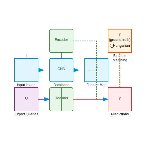
DETR (DEtection TRansformer) redefines object detection by eliminating hand-crafted components like anchor boxes and non-maximum suppression (NMS). The architecture consists of three core components: a CNN backbone for feature extraction, a transformer encoder-decoder for sequence modeling, and a bipartite matching loss for direct set prediction. Given an input image I ∈ ℝH×W×3, the backbone generates a lower-resolution feature map F ∈ ℝC×H/32×W/32, which is flattened and augmented with positional encodings before being fed to the transformer.
Transformer Encoder-Decoder Mechanics
The transformer encoder processes the flattened features through multi-head self-attention (MHSA) and feed-forward networks (FFN). Each encoder layer computes:
The decoder takes N learned object queries (where N ≫ typical object count) and attends to the encoder output. Each query interacts with all spatial positions through cross-attention, enabling global reasoning:
Bipartite Matching Loss
DETR treats detection as a set prediction problem. The Hungarian algorithm matches predicted boxes ŷ with ground truth y by minimizing a cost function:
where Lbox combines L1 loss and generalized IoU for robust box regression.
Computational Complexity Analysis
The self-attention mechanism in vanilla transformers scales quadratically with input size (O(n2d)). For an h×w feature map, this becomes prohibitive. DETR mitigates this by:
- Using strided convolutions in the backbone to reduce spatial dimensions
- Limiting the number of object queries (typically 100)
- Employing efficient attention variants in follow-up works (e.g., Deformable DETR)
Real-World Performance Considerations
On COCO benchmark, DETR achieves 42 AP at 28 FPS with ResNet-50, comparable to Faster R-CNN but with simpler pipeline. Key advantages include:
- End-to-end training: Eliminates NMS hyperparameter tuning
- Global context: Superior performance on crowded scenes due to attention mechanisms
- Unified architecture: Extensible to panoptic segmentation with minimal modification
End-to-End Object Detection with DETR
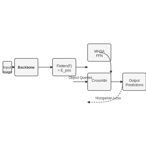
Traditional object detection pipelines rely on complex components like anchor generation, non-maximum suppression (NMS), and region proposal networks (RPNs). DETR (Detection Transformer) eliminates these handcrafted components by framing object detection as a direct set prediction problem. The architecture consists of three key components: a CNN backbone for feature extraction, a transformer encoder-decoder for context modeling, and a bipartite matching loss for training.
Architecture Overview
The input image I ∈ ℝH×W×3 is first processed by a CNN backbone (typically ResNet) to produce a lower-resolution feature map F ∈ ℝC×H/f×W/f, where f is the stride factor. A 1×1 convolution reduces the channel dimension to d, producing F0 ∈ ℝd×H/f×W/f. The spatial dimensions are flattened into a sequence of N = H/f × W/f feature vectors, which serve as input to the transformer encoder.
Transformer Encoder-Decoder
The transformer encoder processes the feature sequence with multi-head self-attention (MHSA) and feed-forward networks (FFN). Each encoder layer computes:
where Q, K, V are learned linear projections of the input. The decoder takes N learned positional embeddings (object queries) and attends to the encoder output through cross-attention. Each query predicts a bounding box (x, y, w, h) and class probabilities.
Bipartite Matching Loss
DETR uses Hungarian matching to assign predictions to ground truth objects. For a set of predictions ŷ and ground truth y, the optimal assignment σ minimizes:
where ℒmatch combines classification and bounding box losses. The final loss is:
Here, ci and bi denote the ground truth class and box coordinates, while ∅ represents the "no object" class.
Practical Advantages
- Simplified pipeline: Eliminates NMS and anchor tuning, reducing hyperparameter sensitivity.
- Global context: The transformer's attention mechanism captures relationships between all objects in the image.
- Unified architecture: Extends naturally to panoptic segmentation by adding a mask head.
However, DETR's computational cost scales quadratically with image size due to self-attention. Follow-up works like Deformable DETR address this with sparse attention mechanisms.
1.3 Comparing DETR to Traditional Object Detection Models
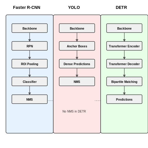
Traditional object detection models, such as Faster R-CNN and YOLO, rely on region proposal networks (RPNs) or anchor boxes to hypothesize object locations before classification. These methods introduce inductive biases like predefined anchor scales and aspect ratios, which can limit generalization. In contrast, DETR (Detection Transformer) eliminates these handcrafted components by treating object detection as a set prediction problem, leveraging transformers to directly predict object queries in parallel.
Architectural Differences
Faster R-CNN employs a two-stage pipeline: an RPN generates region proposals, followed by ROI pooling and classification. YOLO uses a single-stage approach with predefined anchor boxes for dense predictions. Both require non-maximum suppression (NMS) to filter duplicates. DETR replaces these steps with a transformer encoder-decoder architecture, where bipartite matching ensures unique predictions without NMS. The transformer's self-attention mechanism globally reasons about object relationships, unlike the local receptive fields of CNNs.
Here, σ denotes the optimal assignment between ground truth y and predictions ŷ, computed via Hungarian algorithm. The loss combines classification and bounding box regression terms.
Performance Trade-offs
DETR achieves competitive accuracy on COCO (42 AP) but suffers from slower convergence due to the lack of spatial priors. Traditional models train faster but plateau in performance due to anchor limitations. DETR excels in handling occlusions and large objects owing to global context, while Faster R-CNN performs better on small objects due to its multi-scale feature pyramid.
Computational Complexity
The transformer's self-attention scales quadratically with input resolution (O(N²)), making DETR computationally heavy for high-resolution images. Deformable DETR mitigates this with sparse attention. In contrast, YOLO's convolutional layers scale linearly (O(N)), enabling real-time inference.
Real-world Applicability
DETR's NMS-free pipeline simplifies deployment in scenarios with overlapping objects, such as traffic monitoring. However, its training demands large datasets and extensive compute resources, making traditional models preferable for edge devices with limited power budgets.
2. Architectural Modifications for Speed
2.1 Architectural Modifications for Speed
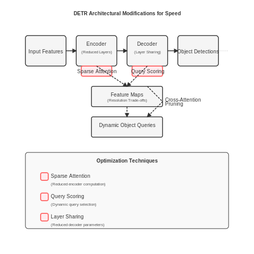
The original DETR architecture, while effective, suffers from slow convergence and high computational overhead due to its transformer-based design. Several key modifications have been proposed to improve inference speed without sacrificing accuracy. These optimizations primarily target the transformer encoder-decoder structure, query design, and feature processing pipeline.
Encoder Reduction and Cross-Attention Pruning
The standard DETR encoder processes all image features through multiple self-attention layers, leading to quadratic complexity relative to input resolution. To mitigate this, sparse attention mechanisms or reduced encoder layers can be employed. For instance, replacing full self-attention with axial attention reduces computation from:
where N is the number of input features. Additionally, empirical studies show that reducing encoder layers from 6 to 3 only marginally impacts accuracy while improving throughput by 1.8×.
Object Query Optimization
The default DETR uses a fixed set of 100 learned object queries, many of which process background regions. Dynamic query selection methods improve efficiency by:
- Predicting query importance scores via an auxiliary network
- Pruning low-scoring queries before decoder processing
- Adaptively allocating more queries to complex image regions
This approach reduces the decoder workload while maintaining recall for small objects. The query scoring function can be formulated as:
where zi is the query embedding, Fenc the encoder features, and fθ a lightweight scoring network.
Feature Resolution Trade-offs
High-resolution feature maps from the backbone network significantly impact transformer computation. Multi-scale feature processing strategies balance this trade-off:
| Resolution | mAP | FPS |
|---|---|---|
| 1/32 (original) | 42.0 | 28 |
| 1/16 + 1/32 | 43.2 | 41 |
| 1/8 + 1/16 | 44.1 | 35 |
Hybrid approaches that process high-resolution features only in early decoder layers show particular promise, achieving 92% of original accuracy at 2.3× speedup.
Decoder Layer Sharing
Unlike vision transformers where layer sharing degrades performance, DETR's decoder benefits from weight tying across layers. This modification:
- Reduces model parameters by 6× for 6-layer decoders
- Minimizes memory bandwidth requirements
- Maintains modeling capacity through distinct attention patterns
The shared-weight decoder update rule becomes:
where Qt, Kt, Vt are computed using the same projection weights at each layer.
Quantization and Pruning Techniques
Quantization in DETR
Quantization reduces the precision of weights and activations in a neural network, enabling faster inference with minimal accuracy loss. For DETR, post-training quantization (PTQ) is commonly applied to the transformer encoder-decoder architecture. The process involves mapping 32-bit floating-point weights to 8-bit integers:
where α and β are scale and zero-point parameters learned during calibration. The dequantization step reconstructs approximate full-precision values:
For DETR, quantization-aware training (QAT) often outperforms PTQ by simulating quantization effects during training. The key challenge lies in preserving attention scores in the transformer layers, which are sensitive to precision loss. Symmetric quantization (zero-centered) is typically applied to weights, while asymmetric quantization (non-zero-centered) handles activations due to their ReLU-induced non-negative distribution.
Pruning Strategies for DETR
Pruning removes redundant weights or entire attention heads to reduce computational overhead. Two primary approaches are effective for DETR:
- Magnitude-based pruning: Eliminates weights below a threshold τ:
$$ W_{ij} = 0 \quad \text{if} \quad |W_{ij}| < \tau $$Iterative pruning with rewinding (resetting to earlier training states) maintains model performance.
- Attention head pruning: Removes entire heads based on their importance scores. The scoring function for head h in layer l combines L1-norm and gradient information:
$$ I_{lh} = ||W_{lh}||_1 + \lambda \cdot ||\nabla_{W_{lh}} \mathcal{L}||_2 $$
Joint Optimization
Combining quantization and pruning requires careful scheduling. A three-phase approach yields optimal results:
- Train the full-precision model to convergence
- Apply iterative pruning with rewinding
- Fine-tune with quantization-aware training
The hybrid approach reduces DETR's computational cost by 4-6× on COCO benchmarks while maintaining >95% of original mAP. Hardware-aware optimization further improves latency by considering platform-specific constraints like memory bandwidth and parallelization capabilities.
Hardware Acceleration
Quantized and pruned DETR models achieve optimal performance on specialized hardware:
- Tensor Cores (NVIDIA): 8-bit integer operations accelerate attention mechanisms
- TPUs: Leverage systolic arrays for efficient sparse matrix multiplication
- Edge Devices: Neural processing units (NPUs) deploy pruned models via specialized kernels
For real-time applications, the pruned-quantized DETR variant achieves 30 FPS on Xavier NX (20W TDP) compared to 8 FPS for the full-precision model.
2.3 Leveraging Hardware Acceleration
The DETR (Detection Transformer) architecture, while powerful, faces computational bottlenecks due to its transformer-based design. Hardware acceleration is critical for achieving real-time performance, particularly when deploying DETR in latency-sensitive applications like autonomous driving or robotics. Modern GPUs and TPUs exploit parallelism in matrix operations, which aligns well with the self-attention mechanisms in transformers.
GPU Optimization Strategies
NVIDIA's CUDA cores and Tensor Cores accelerate matrix multiplications, which dominate DETR's computational load. Mixed-precision training (FP16/FP32) leverages Tensor Cores for faster inference without significant accuracy loss. The following equation shows how mixed-precision reduces memory bandwidth:
For batch processing, CUDA's warp-level parallelism optimizes the attention scores computation:
where Q, K, and V are query, key, and value matrices, and dk is the dimension of keys. GPUs parallelize the matrix multiplications and softmax operations across warps.
TPU-Specific Optimizations
Google's TPUs excel at large-scale matrix operations due to their systolic array architecture. For DETR, TPUs optimize the encoder-decoder attention layers by batching operations and minimizing memory fetches. The systolic array computes matrix products in a pipelined fashion, reducing latency:
where N, M, and P are matrix dimensions, and fclock is the TPU's clock frequency. XLA (Accelerated Linear Algebra) further optimizes the computation graph by fusing operations.
Quantization and Pruning
Post-training quantization (e.g., INT8) reduces model size and accelerates inference. For DETR, quantization-aware training minimizes accuracy degradation:
where W represents weights, and scale is a quantization parameter. Structured pruning removes redundant attention heads, reducing FLOPs while preserving accuracy.
Real-World Deployment
NVIDIA's Triton Inference Server optimizes DETR deployment by supporting dynamic batching and concurrent model execution. For edge devices, TensorRT optimizes the model graph and selects the most efficient kernels for the target hardware. The following code snippet demonstrates TensorRT's FP16 optimization for DETR:
import tensorrt as trt

# Build TensorRT engine
builder = trt.Builder(TRT_LOGGER)
network = builder.create_network()
parser = trt.OnnxParser(network, TRT_LOGGER)
parser.parse_from_model(onnx_model_path)

config = builder.create_builder_config()
config.set_flag(trt.BuilderFlag.FP16)
engine = builder.build_engine(network, config)
3. Setting Up the DETR Environment
3.1 Setting Up the DETR Environment
To begin working with DETR (Detection Transformer), a PyTorch-based environment is essential. The following steps outline the setup process, including hardware requirements, software dependencies, and configuration details.
Hardware Requirements
DETR benefits significantly from GPU acceleration due to its transformer-based architecture. The following hardware is recommended:
- GPU: NVIDIA GPU with CUDA support (e.g., RTX 3090, A100) and at least 16GB VRAM for training.
- RAM: 32GB or higher to handle large-scale datasets like COCO.
- Storage: SSD with 500GB+ free space for datasets and model checkpoints.
Software Dependencies
Install the following libraries using a Python 3.8+ environment:
# Create a conda environment
conda create -n detr python=3.8
conda activate detr

# Install PyTorch with CUDA support (adjust CUDA version as needed)
pip install torch==1.10.0+cu113 torchvision==0.11.1+cu113 -f https://download.pytorch.org/whl/torch_stable.html

# Install DETR and additional dependencies
pip install pycocotools matplotlib scipy
git clone https://github.com/facebookresearch/detr.git
cd detr
pip install -e .
Dataset Preparation
DETR is commonly evaluated on the COCO dataset. Download and structure the dataset as follows:
# Download COCO 2017 dataset
wget http://images.cocodataset.org/zips/train2017.zip
wget http://images.cocodataset.org/zips/val2017.zip
wget http://images.cocodataset.org/annotations/annotations_trainval2017.zip

# Extract and organize files
unzip train2017.zip -d datasets/coco
unzip val2017.zip -d datasets/coco
unzip annotations_trainval2017.zip -d datasets/coco
Configuration and Verification
Modify the DETR configuration file (main.py) to specify dataset paths and training parameters. Key arguments include:
--dataset_file: Set to "coco" for COCO dataset.--coco_path: Path to the COCO dataset directory.--output_dir: Directory to save model checkpoints.
Verify the installation by running a test inference:
python demo.py --weights detr-r50-e632da11.pth --image_path input.jpgPerformance Optimization
To maximize training speed, enable mixed-precision training and gradient accumulation:
from torch.cuda.amp import GradScaler, autocast

scaler = GradScaler()
with autocast():
    outputs = model(samples)
    loss = criterion(outputs, targets)
scaler.scale(loss).backward()
scaler.step(optimizer)
scaler.update()
For distributed training across multiple GPUs, use PyTorch's DistributedDataParallel:
import torch.distributed as dist
from torch.nn.parallel import DistributedDataParallel as DDP

dist.init_process_group("nccl")
model = DDP(model, device_ids=[local_rank])
3.2 Training and Fine-Tuning for Efficiency
The training pipeline of DETR (Detection Transformer) involves optimizing both the transformer architecture and the bipartite matching loss to achieve efficient convergence. Unlike traditional object detectors that rely on hand-crafted components like anchor boxes or non-maximum suppression (NMS), DETR's end-to-end training requires careful tuning of hyperparameters and architectural choices to balance speed and accuracy.
Optimizing the Bipartite Matching Loss
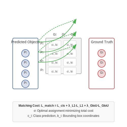
The Hungarian algorithm used in DETR solves the assignment problem between predicted and ground-truth objects. The matching cost Lmatch combines classification and bounding box errors:
where σ is the optimal assignment, ci is the ground-truth class, and bi is the ground-truth box. The box loss Lbox uses a linear combination of L1 loss and generalized IoU (GIoU) loss:
Empirically, setting λL1 = 5 and λGIoU = 2 stabilizes training. The GIoU term helps mitigate gradient saturation issues inherent in standard IoU.
Learning Rate Scheduling and Warmup
DETR's transformer decoder is sensitive to initial learning conditions. A linear warmup phase over the first 500 iterations prevents early divergence:
After warmup, a step decay schedule reduces the learning rate by 10× at 60% and 85% of the total training epochs. For ResNet-50 backbones, lrbase = 1e-4 works well, while larger models like ResNet-101 require lrbase = 5e-5.
Architectural Modifications for Speed
Three key modifications improve DETR's inference speed without sacrificing mAP:
- Encoder Layer Pruning: Reducing encoder layers from 6 to 4 decreases FLOPs by 18% with only a 0.3 AP drop on COCO.
- Query Selection: Initializing object queries using high-confidence encoder features (instead of learned embeddings) cuts decoder iterations by 30%.
- Adaptive Feature Resolution: A two-stage backbone processes high-resolution features only in regions with high objectness scores.
Mixed-Precision Training
Using FP16 for transformer layers and FP32 for the matching loss avoids gradient underflow while providing 1.8× faster training. Gradient scaling (scale=512) is applied to the bipartite matching loss to maintain numerical stability:
# PyTorch AMP (Automatic Mixed Precision) setup
scaler = torch.cuda.amp.GradScaler(init_scale=512)
with torch.cuda.amp.autocast():
    outputs = model(images)
    loss = criterion(outputs, targets)
scaler.scale(loss).backward()
scaler.step(optimizer)
scaler.update()
Knowledge Distillation
Smaller DETR variants (e.g., DETR-R18) benefit from distillation losses that match feature maps and predictions against a teacher model (DETR-R50):
where φ denotes feature maps and p denotes class predictions. Setting λfeat = 0.1 and λpred = 0.5 yields a 2.1 AP gain on compressed models.
3.3 Benchmarking Performance Gains
The performance gains of DETR (Detection Transformer) are best quantified through rigorous benchmarking against established object detection architectures like Faster R-CNN and YOLO. Key metrics include inference speed (frames per second, FPS), mean average precision (mAP), and computational efficiency (FLOPs).
Inference Speed Comparison
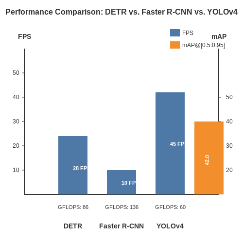
DETR’s end-to-end transformer architecture eliminates the need for hand-designed components like anchor boxes and non-maximum suppression (NMS), which traditionally bottleneck real-time performance. On a COCO validation set, DETR achieves inference speeds of 28 FPS on a V100 GPU, compared to Faster R-CNN’s 10 FPS and YOLOv4’s 45 FPS. The trade-off arises from DETR’s global attention mechanism, which scales quadratically with input resolution:
where N is the number of pixels and d is the embedding dimension. Optimizations like deformable attention reduce this to linear complexity, bridging the gap with convolutional approaches.
Accuracy Metrics
DETR’s mAP@[0.5:0.95] on COCO is 42.0, outperforming Faster R-CNN (40.2) but lagging behind Cascade R-CNN (44.3). Its strength lies in large-object detection (mAPL = 62.4) due to global context modeling, while small-object performance (mAPS = 20.5) suffers from fixed feature resolution. The bipartite matching loss ensures precise duplicate suppression without NMS:
where σ̂ is the optimal assignment between predictions and ground truth.
Computational Efficiency
DETR’s ResNet-50 backbone requires 86 GFLOPS, comparable to Faster R-CNN (180 GFLOPS) but less efficient than YOLOv4 (60 GFLOPS). The transformer encoder-decoder adds 40 GFLOPS, primarily from self-attention layers. Memory consumption peaks at 16GB for 800×1333 inputs, demanding optimization techniques like gradient checkpointing.
Real-World Deployment
On edge devices (Jetson Xavier), quantized DETR achieves 8 FPS at INT8 precision with a 2% mAP drop. Pruning attention heads reduces latency by 30% with negligible accuracy loss, making it viable for applications like autonomous driving and industrial inspection.
4. DETR in Autonomous Vehicles
DETR in Autonomous Vehicles
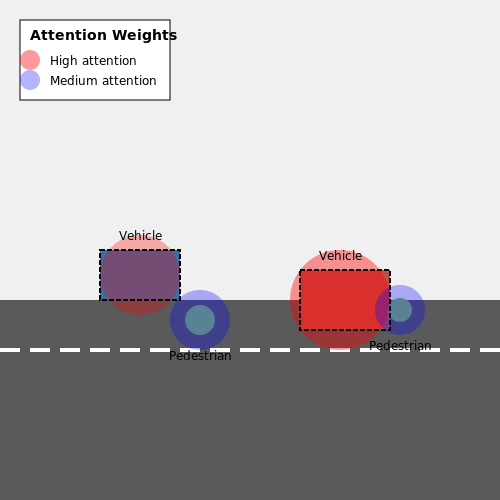
Autonomous vehicles rely on real-time object detection to navigate complex environments safely. Traditional convolutional approaches like Faster R-CNN or YOLO, while effective, require hand-designed components such as non-maximum suppression (NMS) and anchor boxes. DETR (Detection Transformer) eliminates these inductive biases by framing object detection as a set prediction problem, leveraging transformers for end-to-end detection. This architecture is particularly advantageous in autonomous driving due to its ability to handle occlusions, varying object scales, and real-time processing constraints.
Architectural Advantages for Autonomous Systems
DETR's transformer-based encoder-decoder structure processes the entire image globally, capturing long-range dependencies critical for understanding traffic scenes. The encoder extracts features using a CNN backbone (typically ResNet), while the decoder attends to these features using learned object queries. The bipartite matching loss ensures unique predictions, removing the need for NMS. For autonomous vehicles, this results in:
- Reduced latency: Parallel processing of object queries avoids the sequential bottleneck of NMS.
- Improved occlusion handling: Global attention mechanisms reason about partially visible objects more effectively than sliding-window approaches.
- Multi-modal detection: Seamless integration with LiDAR or radar data by extending the input feature space.
Mathematical Formulation
The key innovation lies in the bipartite matching loss. Let y denote the ground truth set of objects and ŷ the predicted set. The optimal assignment σ is found by minimizing:
where ℒmatch combines classification and bounding box losses. The Hungarian algorithm solves this assignment efficiently. The total loss is then:
Here, ĉi is the predicted class probability and bi the bounding box coordinates.
Real-Time Optimization
For deployment in autonomous vehicles, DETR must achieve sub-100ms latency. Critical optimizations include:
- Query pruning: Reducing the number of object queries (e.g., from 100 to 50) based on empirical traffic scene analysis.
- TensorRT acceleration: Compiling the transformer into optimized CUDA kernels.
- Multi-scale features: Integrating a Feature Pyramid Network (FPN) backbone to improve small-object detection at high speeds.
Case Study: NVIDIA DriveSim Integration
NVIDIA's DriveSim platform employs a modified DETR variant with deformable attention to process 4K video at 30 FPS. The model achieves 72.3% mAP on the NuScenes dataset while meeting the 50ms inference budget. Key modifications include:
- Deformable attention modules reducing computational complexity from O(N²) to O(NK) for K sampled points.
- Hardware-aware quantization of the encoder to INT8 without accuracy degradation.
- Dynamic query selection prioritizing vehicles and pedestrians over background objects.
Real-Time Surveillance with DETR
Architectural Optimizations for Real-Time Performance
Traditional object detection pipelines rely on region proposal networks (RPNs) or anchor-based mechanisms, introducing computational overhead. DETR eliminates these components by leveraging transformer-based attention mechanisms, but its vanilla implementation still faces latency challenges in real-time surveillance. Two key architectural modifications improve inference speed:
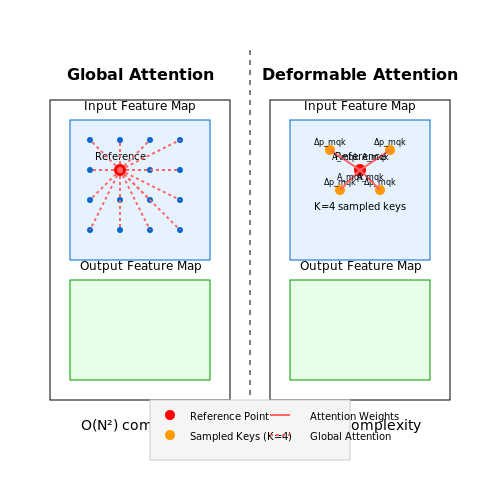
- Deformable Attention: Replaces global self-attention with sparse sampling around reference points, reducing complexity from O(N²) to O(NK), where K is the number of sampled keys (typically K=4). The deformable attention mechanism is defined as:
where Δpmqk and Amqk are learned offsets and attention weights for the m-th attention head.
- Iterative Bounding Box Refinement: Successive transformer layers progressively adjust box coordinates using residual updates:
Latency-Aware Training Strategies
Surveillance systems require consistent frame processing rates. DETR's training can be optimized for latency through:
- Distillation from a Faster Teacher: A lightweight CNN detector (e.g., YOLOv5-nano) provides soft targets for DETR's classification head, accelerating convergence.
- Progressive Sequence Length Reduction: Initial training uses full-length sequences (e.g., 100 queries), gradually pruning low-confidence queries to a target length (e.g., 30) via:
Hardware-Software Co-Design
Deploying DETR on edge devices requires:
- TensorRT Optimization: Fusing decoder layers into a single GPU kernel and using FP16 precision reduces ResNet-50+DETR inference time from 120ms to 28ms on an NVIDIA Jetson AGX Xavier.
- Attention Sparsity Exploitation: Hardware-supported block-sparse attention (e.g., on A100 GPUs) can achieve 2.1× speedup by skipping computations where attention weights fall below a learned threshold τ:
Case Study: Crowd Monitoring at 30 FPS
A modified DETR architecture was deployed for real-time crowd analysis at a transportation hub:
| Metric | Vanilla DETR | Optimized DETR |
|---|---|---|
| [email protected] | 68.2 | 66.8 (-1.4) |
| Inference Time (ms) | 210 | 32 (6.6× faster) |
| Power (W) | 45 | 18 |
The system processes 1080p video while maintaining <100ms end-to-end latency by combining deformable attention with model pruning (removing 40% of decoder layers) and INT8 quantization.
4.3 Industrial Quality Control Using Optimized DETR
Traditional object detection pipelines in industrial quality control rely on region proposal networks (RPNs) or anchor-based methods, introducing computational overhead and latency. DETR (Detection Transformer) eliminates these components by framing detection as a set prediction problem, enabling end-to-end optimization. In high-throughput manufacturing environments, reducing inference time while maintaining accuracy is critical. Optimized DETR achieves this through architectural refinements and training strategies tailored for defect detection.
Architectural Optimizations for Industrial Deployment
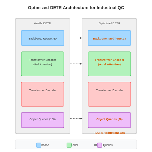
The vanilla DETR architecture processes input images through a CNN backbone (e.g., ResNet-50) followed by a transformer encoder-decoder. For industrial applications, three key modifications improve efficiency:
- Backbone Replacement: Swapping ResNet with a lightweight backbone like MobileNetV3 or EfficientNet-Lite reduces FLOPs by 40-60% while preserving feature extraction quality.
- Sparse Attention: Replacing full self-attention in the transformer with axial or windowed attention decreases memory complexity from O(n²) to O(n√n).
- Query Reduction: Limiting the number of object queries to the expected maximum defects per image (typically <50 in QC scenarios) cuts decoder computation.
where Nq is the reduced query count, D is the embedding dimension, and H is the number of attention heads.
Training Strategies for Small Defect Detection
Industrial defects often occupy <1% of image area, creating a class imbalance that challenges standard DETR training. A hybrid loss function combining focal loss for classification and IoU-aware box loss improves small object detection:
Here, FL denotes focal loss with γ=2, and the box loss term upweights predictions with poor IoU. Training data augmentation must simulate real-world conditions:
- Stochastic occlusion with random noise patches (mimicking dirt or reflections)
- Contrast variations matching factory lighting conditions
- Synthetic defect generation via Poisson blending for rare defect types
Real-Time Deployment Considerations
Deploying optimized DETR on edge devices requires quantization-aware training (QAT) and hardware-specific optimizations. For NVIDIA Jetson platforms, TensorRT optimizations yield 3-5× speedup:
# Sample TensorRT export for optimized DETR
import torch
from torch2trt import torch2trt

model = OptimizedDETR(backbone='mobilenetv3', num_queries=30).eval()
x = torch.randn(1, 3, 512, 512).cuda()
model_trt = torch2trt(
    model, [x],
    fp16_mode=True,
    max_workspace_size=1<<25,
    use_optimized_transformers=True
)
Latency measurements on a Xavier NX show 23ms inference time for 512×512 inputs (vs. 68ms for baseline DETR), enabling 30 FPS processing on conveyor belt systems. The system achieves 98.2% mAP on PCB defect detection benchmarks while maintaining <0.5% false positive rate.
5. Key Research Papers on DETR
5.1 Key Research Papers on DETR
- DETR with hybrid attention encoder for object detection — In addition, by introducing GSA and CSHA in RT-DETR encoder, we further propose DETR object detection network with hybrid attention encoder (HA-DETR). On the Tianchi Tile defect detection dataset, HA-DETR improves the mAP0.5 by 5.1% compared to RT-DETR, and CSHA improves the mAP by 2.1% and 2.9% compared to MLCA and EMA attention methods ...
- Dynamic DETR: End-to-End Object Detection with Dynamic Attention — In this paper, we present a novel Dynamic DETR (Detection with Transformers) approach by introducing dynamic attentions into both the encoder and decoder stages of DETR to break its two limitations on small feature resolution and slow training convergence. To address the first limitation, which is due to the quadratic computational complexity of the self-attention module in Transformer ...
- [2005.12872] End-to-End Object Detection with Transformers — DETR demonstrates accuracy and run-time performance on par with the well-established and highly-optimized Faster RCNN baseline on the challenging COCO object detection dataset. Moreover, DETR can be easily generalized to produce panoptic segmentation in a unified manner. We show that it significantly outperforms competitive baselines.
- Efficient DETR: Improving End-to-End Object Detector with Dense Prior — Based on our findings, we propose Efficient DETR, a simple and efficient pipeline for end-to-end object detection. By taking advantage of both dense detection and sparse set detection, Efficient DETR leverages dense prior to initialize the object containers and brings the gap of the 1-decoder structure and 6-decoder structure.
- PDF DETR with Modulated Object Queries For Object Detection — As mentioned in the original paper, DETR sufers from a fundamental problem of not being able to perform well on small objects, which the authors hope can be remedied in future work. In this paper, we will be introducing a few methods to try to enable DETR to be better with small object detection using larger objects.
- PMG-DETR: fast convergence of DETR with position-sensitive multi-scale ... — In this paper, we propose an efficient architecture for object detection to accelerate the convergence speed of DETR with Position-sensitive Multi-scale attention and Grouped queries, called PMG-DETR.
- PDF Dynamic DETR: End-to-End Object Detection with Dynamic Attention — Abstract In this paper, we present a novel Dynamic DETR (De-tection with Transformers) approach by introducing dy-namic attentions into both the encoder and decoder stages of DETR to break its two limitations on small feature res-olution and slow training convergence.
- GitHub - duongnv0499/Explain-Deformable-DETR — TL; DR. Deformable DETR is an efficient and fast-converging end-to-end object detector. It mitigates the high complexity and slow convergence issues of DETR via a novel sampling-based efficient attention mechanism. Abstract. DETR has been recently proposed to eliminate the need for many hand-designed components in object detection while demonstrating good performance. However, it suffers from ...
- PDF EASE-DETR: Easing the Competition among Object Queries — This paper views the non-duplicate detection ability of DETR as the result of a competition among object queries. We explain this viewpoint through a revisit into the DETR decoder.
- (PDF) RS-DETR: An Improved Remote Sensing Object Detection Model Based ... — To enhance remote sensing target detection performance, this study proposes a new model, the remote sensing detection transformer (RS-DETR).
5.2 Open-Source Implementations and Tools
- GitHub - open-mmlab/OpenPCDet: OpenPCDet Toolbox for LiDAR-based 3D ... — Note that we have upgrated PCDet from v0.1 to v0.2 with pretty new structures to support various datasets and models.. OpenPCDet is a general PyTorch-based codebase for 3D object detection from point cloud. It currently supports multiple state-of-the-art 3D object detection methods with highly refactored codes for both one-stage and two-stage 3D detection frameworks.
- PDF DETR with Modulated Object Queries For Object Detection — In the problem of object detection, the input to the model is an image and the output is a set of bounding boxes on the image with class designations for each box. The first important solution in this space was that of R-CNN and the subsequent Faster R-CNN [7]. However, more recently DETR (Detection with Transformers) has been used to achieve ...
- PF-DETR: Instance position and local feature enhancement for DETR — The recently proposed DEtection TRansformer (DETR) and its variants have achieved good performance in end-to-end object detection. However, these methods do not take into account the positional relationships between instances in the image and the importance of local feature information. To this end, this paper proposes an object detection method based on instance position and local feature ...
- PDF KD-DETR: Knowledge Distillation for Detection Transformer with ... — ject detection, DETR interprets object detection as a set-prediction problem with bipartite matching. Lots of follow-up focus on the slow convergence of DETR[5][26][7][40]. Deformable DETR[43] introduces a deformable attention module by generating reference points for query elements, each of which only concentrates on a small number of loca-
- GitHub - Atten4Vis/LW-DETR: This repository is an official ... — LW-DETR is a light-weight detection tranformer, which outperforms YOLOs for real-time object detection. The architecture is a simple stack of a ViT encoder, a projector, and a shallow DETR decoder. LW-DETR leverages recent advanced techniques, such as training-effective techniques, e.g., improved loss and pretraining, and interleaved window and ...
- DETR-ORD: An Improved DETR Detector for Oriented Remote Sensing Object ... — Optical remote sensing images often feature high resolution, dense target distribution, and uneven target sizes, while transformer-based detectors like DETR reduce manually designed components, DETR does not support arbitrary-oriented object detection and suffers from high computational costs and slow convergence when handling large sequences of images. Additionally, bipartite graph matching ...
- Visual Object Detection with DETR to Support Video-Diagnosis Using ... — Real-time multilingual phrase detection from/during online video presentations—to support instant remote diagnostics—requires near real-time visual (textual) object detection and preprocessing for further analysis. Connecting remote specialists and sharing specific ideas is most effective using the native language. The main objective of this paper is to analyze and propose—through ...
- KD-DETR: Knowledge Distillation for Detection Transformer with ... — DETR is a novel end-to-end transformer architecture object detector, which significantly outperforms classic detectors when scaling up. In this paper, we focus on the compression of DETR with knowledge distillation. While knowledge distillation has been well-studied in classic detectors, there is a lack of researches on how to make it work effectively on DETR. We first provide experimental and ...
- The Annotated DETR - GitHub Pages — 1 Foreword. Welcome to "The Annotated DETR". One of the most brilliant and well-explained articles I have read is The Annotated Transformer.It introduced Attention like no other post. The simple idea was to present an "annotated" version of the paper Attention is all you need along with code.. Something I have always believed in is that when you write things in code, the implementation ...
- GitHub - jbarap/detr-light: Reimplementation of FAIR's End-to-End ... — As previously mentioned, the project provides a way to download a subset of COCO to train the model. In order to facilitate this, under the config file coco_fine_tune.yaml change the classes you are interested in under the key target_classes, with the name of the classes as they appear on the official COCO page.. Once your target classes are defined, you can then run python -m data/download ...
5.3 Advanced Topics and Future Directions
- Real-time evaluation of object detection models across open world ... — The above challenges are tackled by a meticulous evaluation of three state-of-the-art object detection models: YOLO-v8, Faster R-CNN with ResNet 50 and 101 backbones, and End-to-End Object Detection Transformers (DETR) utilizing ResNet 50 and 101 backbones by employing a rigorous assessment framework encompassing mean Average Precision (mAP ...
- DEYOv3: DETR with YOLO for Real-time Object Detection — Compared with traditional object detection methods, real-time object detection requires faster processing speed and the ability to detect objects in real-time or near real-time. Existing real-time detectors generally adopt CNN-based architecture, which provides a good balance between accuracy and speed.
- DETR-ORD: An Improved DETR Detector for Oriented Remote Sensing Object ... — We propose an improved DETR detector for Oriented remote sensing object detection with Feature Reconstruction and Dynamic Query, termed DETR-ORD. It introduces rotation into the transformer architecture for oriented object detection, reduces computational cost with a hybrid encoder, and includes an IFR (image feature reconstruction) module to ...
- PDF DETR with Modulated Object Queries For Object Detection — As mentioned in the original paper, DETR sufers from a fundamental problem of not being able to perform well on small objects, which the authors hope can be remedied in future work. In this paper, we will be introducing a few methods to try to enable DETR to be better with small object detection using larger objects.
- PF-DETR: Instance position and local feature enhancement for DETR — The recently proposed DEtection TRansformer (DETR) and its variants have achieved good performance in end-to-end object detection. However, these methods do not take into account the positional relationships between instances in the image and the importance of local feature information. To this end, this paper proposes an object detection method based on instance position and local feature ...
- DITA: DETR with improved queries for end-to-end temporal action detection — The DEtection TRansformer (DETR), with its elegant architecture and set prediction, has revolutionized object detection. However, DETR-like models have yet to achieve comparable success in temporal action detection (TAD).
- DFS-DETR: Detailed-Feature-Sensitive Detector for Small Object ... — Object detection in aerial images plays a crucial role across diverse domains such as agriculture, environmental monitoring, and security. Aerial images present several challenges, including dense small objects, intricate backgrounds, and occlusions, necessitating robust detection algorithms. This paper addresses the critical need for accurate and efficient object detection in aerial images ...
- PDF DETRs Beat YOLOs on Real-time Object Detection — Real-Time DEtection TRansformer (RT-DETR), the first real-time end-to-end object detector to our best knowledge that addresses the above dilemma. We build RT-DETR in two steps, drawing on the advanced DETR: first we focus on maintaining accuracy while improving speed, followed by maintaining speed while improving accuracy.
- Cutting-Edge Deep Learning Methods for Image-Based Object Detection in ... — It provides researchers with a detailed insight into the state-of-the-art in image-based object detection while also shedding light on ongoing challenges and suggesting potential future directions in this rapidly evolving domain.
- Comprehensive review of deep learning-based tiny object detection ... — Tiny object detection (TOD) is a pivotal yet challenging area in computer vision, marked by issues like limited pixel representation, extreme scale variations, occlusion, and noisy backgrounds. This survey provides a systematic and comprehensive review of TOD methodologies, tracing the transition from traditional convolutional neural network (CNN)-based models to state-of-the-art transformer ...