1.1 Historical Context and Motivation for Transformers

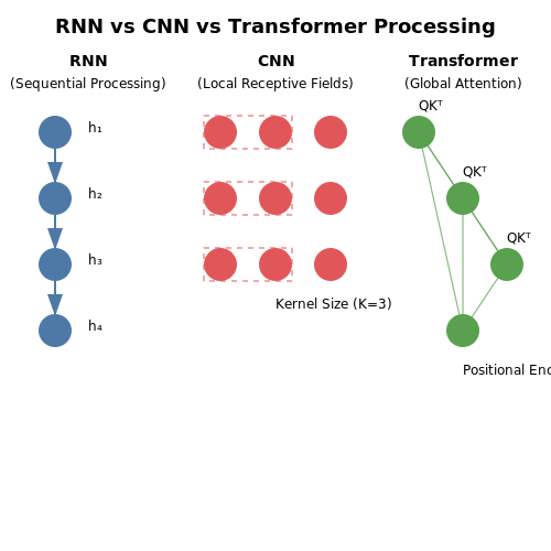
Prior to the introduction of transformers in 2017, sequence modeling and transduction tasks were dominated by recurrent neural networks (RNNs) and convolutional neural networks (CNNs). While effective, these architectures suffered from fundamental limitations in handling long-range dependencies and parallelization. RNNs, including Long Short-Term Memory (LSTM) and Gated Recurrent Unit (GRU) variants, process sequences sequentially, making them inherently slow to train due to their temporal dependency. The vanishing gradient problem further restricted their ability to capture relationships between distant tokens in long sequences.

CNNs, when applied to sequence tasks, could process inputs in parallel through dilated convolutions. However, they required increasingly large receptive fields to model long-range dependencies, leading to computational inefficiency. The number of operations needed to relate two positions grew linearly or logarithmically with distance, making it difficult to learn direct relationships between arbitrary positions in the input and output sequences.

The Attention Mechanism Breakthrough

The key innovation that enabled transformers was the attention mechanism, first introduced for neural machine translation in 2014. The original formulation computed a weighted sum of encoder hidden states at each decoder step, allowing the model to dynamically focus on relevant parts of the input sequence. This proved more effective than fixed-length vector representations used in earlier encoder-decoder architectures.

The 2017 paper Attention Is All You Need by Vaswani et al. took this concept further by eliminating recurrence entirely. The transformer architecture replaced sequential processing with self-attention mechanisms that could directly model relationships between all positions in the input and output sequences with a constant number of operations. This was achieved through three key mathematical operations:

Where Q (queries), K (keys), and V (values) are learned linear transformations of the input embeddings, and d_k is the dimension of the keys. The scaling factor 1/√d_k prevents dot products from growing too large in magnitude, which would push the softmax into regions with extremely small gradients.

Parallelization and Computational Efficiency

The transformer's architecture enabled unprecedented parallelization during training. Unlike RNNs that require sequential computation of hidden states, self-attention layers can process all positions simultaneously. This property, combined with modern GPU/TPU architectures, reduced training times from weeks to days for comparable model sizes. The computational complexity of self-attention is:

Where n is the sequence length and d is the representation dimension. While quadratic in sequence length, this proved more efficient in practice than the O(n) sequential operations of RNNs due to massive parallelization and optimized matrix multiplication routines.

Positional Encoding and Sequence Modeling

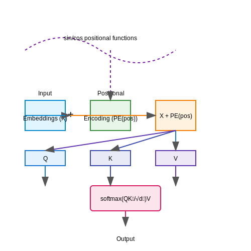
Since transformers lack inherent notion of sequence order, they incorporate positional encodings to inject information about token positions. The original paper used sinusoidal functions of varying frequencies:

Where pos is the position and i is the dimension. This choice allows the model to learn to attend by relative positions, as any fixed offset k, PE_pos+k can be represented as a linear function of PE_pos.

Impact on Modern AI Systems

The transformer architecture's scalability led to rapid adoption across natural language processing, with models like BERT, GPT, and T5 achieving state-of-the-art results on numerous benchmarks. Its success subsequently extended to computer vision (Vision Transformers), speech processing, and multimodal systems. The attention mechanism's ability to model arbitrary dependencies between input and output positions, regardless of distance, fundamentally changed the approach to sequence modeling across AI domains.

1.2 Key Innovations: Self-Attention and Positional Encoding

Self-Attention Mechanism

The self-attention mechanism is the cornerstone of the Transformer architecture, enabling the model to weigh the importance of different input tokens dynamically. Unlike traditional recurrent or convolutional approaches, self-attention computes pairwise interactions between all tokens in a sequence, capturing long-range dependencies without sequential processing.

Given an input sequence of embeddings X ∈ ℝ^n×d, where n is the sequence length and d is the embedding dimension, self-attention projects X into three matrices:

where W_Q, W_K, W_V ∈ ℝ^d×d_k are learnable weight matrices. The attention scores are computed as scaled dot-products between queries Q and keys K:

The scaling factor √d_k prevents gradient vanishing issues caused by large dot-product magnitudes. Multi-head attention extends this by running h parallel attention heads, concatenating their outputs:

where each head performs independent attention computations with different learned projections.

Positional Encoding

Since self-attention is permutation-invariant, positional encodings are added to input embeddings to inject information about token order. The original Transformer uses sinusoidal positional encodings defined as:

where pos is the position and i is the dimension index. This encoding scheme allows the model to attend to relative positions through linear transformations, as shown by the trigonometric identity:

where T_k is a linear transformation matrix dependent on k. Recent variants like learned positional embeddings or relative position representations (e.g., Shaw et al., 2018) have shown improved performance in certain tasks.

Practical Implications

The combination of self-attention and positional encoding enables three key advantages:

• Parallelization: Unlike RNNs, all attention scores can be computed simultaneously.
• Long-range dependency capture: Direct token-to-token interactions mitigate vanishing gradients in long sequences.
• Interpretability: Attention weights often reveal linguistically meaningful patterns (e.g., coreference resolution).

In practice, modern implementations optimize memory usage through techniques like memory-efficient attention (Rabe and Staats, 2021) or flash attention (Dao et al., 2022) to handle sequences exceeding 32K tokens.

Comparison with RNNs and CNNs: Why Transformers?

Recurrent Neural Networks (RNNs) and Their Limitations

RNNs process sequential data through recurrent connections, maintaining a hidden state that theoretically captures information from all previous time steps. The core recurrence relation is:

where h_t is the hidden state at time t, x_t is the input, and W_h, W_x are learnable weights. While elegant in theory, RNNs suffer from two critical weaknesses:

• Vanishing/exploding gradients: The repeated multiplication of W_h makes learning long-range dependencies practically impossible without careful initialization or architectural modifications.
• Sequential computation: The inherently sequential nature prevents parallelization during training, making RNNs prohibitively slow for long sequences.

Convolutional Neural Networks (CNNs) for Sequences

CNNs apply learned filters across temporal or spatial dimensions, with the 1D temporal convolution operation defined as:

where w_k are the filter weights and K is the kernel size. While CNNs offer:

• Parallel computation: Unlike RNNs, convolutions can be computed simultaneously across all positions.
• Local feature extraction: Effective for capturing local patterns through hierarchical layers.

They still struggle with:

• Fixed receptive fields: Capturing long-range dependencies requires either very large kernels or many stacked layers, increasing computational cost.
• Positional invariance: Standard convolutions are translation-equivariant, which may not be ideal for tasks where absolute position matters.

The Transformer Advantage

Transformers address these limitations through two key innovations:

1. Self-Attention Mechanism

The scaled dot-product attention computes pairwise relationships between all positions in constant time:

where Q, K, V are learned query, key, and value matrices. This provides:

• Global receptive field: Any two positions can directly interact, regardless of distance.
• Dynamic feature weighting: Attention weights adaptively highlight relevant relationships.

2. Parallel Sequence Processing

Unlike RNNs, Transformers process all positions simultaneously through:

• Positional encodings: Injected sinusoidal or learned vectors preserve sequence order:

• Layer normalization and residual connections: Enable stable training of deep architectures.

Empirical Performance Comparison

On the WMT 2014 English-to-German translation task:

The Transformer achieves superior performance with significantly faster training, demonstrating the architectural advantages in both quality and computational efficiency.

Self-Attention Mechanism: Scaled Dot-Product Attention

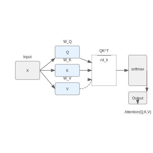
The scaled dot-product attention mechanism forms the core of transformer architectures, enabling dynamic weighting of input tokens based on their contextual relationships. Given an input sequence of embeddings X ∈ ℝ^n×d, where n is sequence length and d is embedding dimension, the mechanism first projects X into three learned matrices:

Here W_Q, W_K ∈ ℝ^d×d_k and W_V ∈ ℝ^d×d_v are projection matrices for queries, keys, and values respectively. The attention scores are computed as scaled dot-products between queries and keys:

Mathematical Derivation

The scaling factor 1/√d_k is critical for stable gradient propagation. For high-dimensional keys, the dot product QK^T grows large in magnitude, pushing softmax outputs into saturated regions. The scaling preserves gradient flow:

where q_i and k_j are random vectors with unit variance components. This maintains stable gradients regardless of d_k.

Parallel Computation

The mechanism computes attention scores for all positions simultaneously via batched matrix multiplication. For a sequence of length n, the attention pattern forms an n×n matrix where each row sums to 1 after softmax normalization. This allows modeling arbitrary token-to-token dependencies.

Multi-Head Extension

Multi-head attention splits the projections into h parallel heads:

Each head applies independent attention in reduced dimension spaces (typically d_k = d_v = d/h), enabling specialized attention patterns across different representation subspaces.

Computational Complexity

The dominant term is the QK^T multiplication with O(n²d) complexity. While effective for moderate sequence lengths, this quadratic scaling motivates research into sparse attention variants for long sequences.

Multi-Head Attention: Parallel Processing of Attention Heads

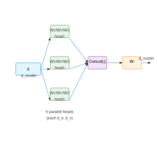
The multi-head attention mechanism extends single-head attention by computing multiple attention operations in parallel, allowing the model to jointly attend to information from different representation subspaces. Each attention head operates independently with its own set of learnable parameters, enabling the model to capture diverse relationships in the input sequence.

Mathematical Formulation

Given an input sequence X of dimension n × d_model, multi-head attention first projects X into h different sets of queries, keys, and values using learned linear transformations:

where W_i^Q ∈ ℝ^{d_model × d_k}, W_i^K ∈ ℝ^{d_model × d_k}, and W_i^V ∈ ℝ^{d_model × d_v} are the projection matrices for head i, with d_k = d_v = d_model/h.

Parallel Attention Computation

Each head computes scaled dot-product attention independently:

The outputs of all heads are concatenated and linearly transformed to produce the final multi-head attention output:

where W^O ∈ ℝ^{hd_v × d_model} is the output projection matrix.

Advantages of Multi-Head Attention

• Diverse Representation Learning: Different heads can learn to attend to different aspects of the input (e.g., syntactic vs. semantic relationships).
• Improved Gradient Flow: Parallel computation allows for more efficient backpropagation through multiple attention pathways.
• Scalability: The computational complexity remains O(n²d) while providing h times more representational capacity.

Implementation Considerations

In practice, multi-head attention is implemented efficiently using batch matrix operations. For h heads, the projections can be computed as a single large matrix multiplication:

The resulting tensor is then split into h heads along the feature dimension. This approach maximizes GPU utilization by avoiding sequential computation of individual heads.

Empirical Observations

Research has shown that different heads often specialize in distinct patterns:

• Some heads attend to local syntactic patterns (e.g., verb-object relationships)
• Others capture long-range dependencies or positional relationships
• A subset of heads may act as "noise" filters or redundancy handlers

The number of heads h is typically chosen such that d_k = d_v = d_model/h remains large enough to maintain meaningful representations (common values are 8-16 heads for d_model=512).

Position-wise Feed-Forward Networks

Each position in the Transformer's self-attention output undergoes an identical transformation through a position-wise feed-forward network (FFN). Despite its name, the FFN is applied independently and identically to each position, making it position-wise rather than sequential. This design allows parallel processing across all positions while introducing non-linearity and increased model capacity.

Mathematical Formulation

The FFN consists of two linear transformations with a ReLU activation in between:

Where:

• x ∈ ℝ^d_model is the input vector (d_model = 512 in the original Transformer)
• W₁ ∈ ℝ^{d_model × d_ff} and W₂ ∈ ℝ^{d_ff × d_model} are learnable weights
• d_ff is the inner layer dimensionality (typically 2048 or 4096)
• The ReLU activation (max(0,·)) introduces non-linearity

Architectural Properties

The FFN serves several critical functions:

• Dimensionality expansion: The hidden layer (d_ff) is typically 4× wider than d_model, enabling richer representations
• Non-linear transformation: The ReLU activation allows modeling complex interactions that the attention mechanism alone cannot capture
• Position independence: Unlike RNNs, the same weights are applied to all positions, making the operation fully parallelizable

Variants and Improvements

Several modifications to the original FFN have been proposed:

Gated Linear Units (GLU)

Used in models like PaLM and GPT-3, replacing ReLU with a gating mechanism:

where σ is the sigmoid function and ⊗ denotes element-wise multiplication.

SwiGLU Activation

Combining Swish activation with GLU, as used in LLaMA and GPT-4:

Computational Considerations

The FFN typically accounts for about 2/3 of the Transformer's total parameters and FLOPs. For a model with d_model = 1024 and d_ff = 4096:

Modern implementations often fuse the two linear transformations into a single optimized kernel for efficiency.

Layer Normalization and Residual Connections

Layer Normalization in Transformers

Layer normalization (LayerNorm) is a critical component in Transformer architectures, stabilizing training by normalizing activations across the feature dimension. Unlike batch normalization, which operates over the batch dimension, LayerNorm computes statistics independently for each sample, making it suitable for variable-length sequences common in NLP tasks. Given an input vector x of dimension d, LayerNorm applies:

where μ and σ² are the mean and variance of x, γ and β are learnable scale and shift parameters, and ϵ is a small constant for numerical stability. This operation ensures that gradients remain well-conditioned during backpropagation, mitigating the vanishing gradient problem in deep networks.

Residual Connections

Residual connections, introduced in ResNet, are employed in Transformers to enable training of very deep networks. They allow gradients to flow directly through the network via identity mappings, preserving information across layers. For a sublayer F (e.g., attention or feed-forward), the output is computed as:

This additive skip connection ensures that even if F(x) becomes small during initialization, the network can still propagate meaningful signals. Combined with LayerNorm, the standard Transformer layer implements this as:

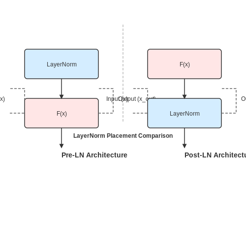
Pre-LN vs. Post-LN Architectures

Recent variants of Transformers debate the placement of LayerNorm. In the original Post-LN architecture, LayerNorm is applied after the residual connection:

In Pre-LN architectures, LayerNorm is applied before the sublayer:

Pre-LN tends to enable more stable training for very deep networks, as gradients flow more smoothly through the normalization layers. Empirical studies show Pre-LN achieves faster convergence but may sacrifice peak performance in some tasks.

Gradient Flow Analysis

The effectiveness of residual connections can be analyzed through gradient propagation. Let L be the loss function. The gradient of L with respect to the input x of a residual block is:

This decomposition shows that the identity term I ensures gradients can propagate directly, even when the Jacobian ∂F(x)/∂x becomes small. LayerNorm further stabilizes this by bounding the magnitude of activations entering F.

Practical Implications

In modern implementations like GPT-3 and BERT, LayerNorm and residual connections are applied per transformer block. Key design choices include:

• Initialization: Scale parameters γ in LayerNorm are initialized to 1, while β is initialized to 0.
• Precision: LayerNorm is sensitive to numerical precision, often requiring float32 in practice.
• Parallelism: Residual connections enable model parallelism by allowing independent computation of F(x) across devices.

Encoder-Decoder Structure: Roles and Responsibilities

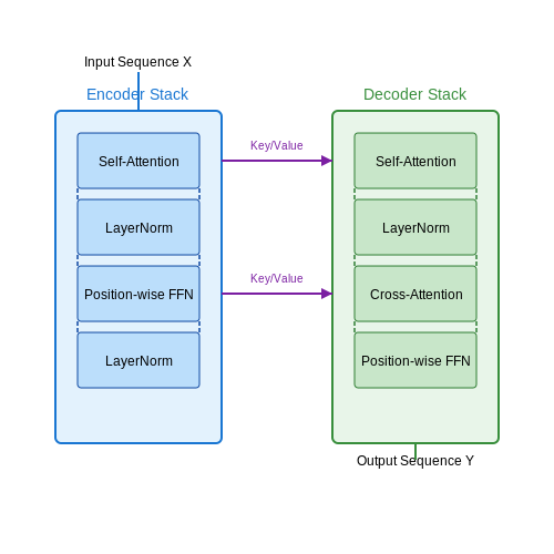
The encoder-decoder architecture forms the backbone of the original Transformer model, as introduced in Attention Is All You Need (Vaswani et al., 2017). This structure is particularly effective for sequence-to-sequence (seq2seq) tasks such as machine translation, text summarization, and dialogue generation, where an input sequence is transformed into an output sequence of potentially different length.

Encoder: Feature Extraction and Contextual Representation

The encoder processes the input sequence $$X = (x_1, x_2, ..., x_n)$$ through a stack of N identical layers (typically N = 6 in the original paper). Each layer consists of two sub-layers:

• Multi-Head Self-Attention: Computes attention scores between all pairs of tokens in the input sequence, enabling the model to weigh the importance of each token relative to others. The output is a weighted sum of value vectors, where weights are determined by the compatibility of queries and keys.
• Position-wise Feed-Forward Network: A two-layer MLP with ReLU activation, applied independently to each token position. This introduces non-linearity and allows the model to transform features in a position-specific manner.

Both sub-layers employ residual connections followed by layer normalization, formalized as:

The encoder's output is a sequence of continuous representations $$Z = (z_1, z_2, ..., z_n)$$, where each $$z_i$$ encodes contextual information from the entire input sequence.

Decoder: Autoregressive Generation with Masked Attention

The decoder generates the output sequence $$Y = (y_1, y_2, ..., y_m)$$ one token at a time in an autoregressive manner. Each decoder layer includes three sub-layers:

• Masked Multi-Head Self-Attention: Similar to the encoder's self-attention but with a masking mechanism to prevent positions from attending to subsequent tokens, ensuring the model only uses information from previously generated outputs during training.
• Multi-Head Cross-Attention: Queries from the decoder attend to keys and values from the encoder's output $$Z$$, aligning decoder states with relevant input context.
• Position-wise Feed-Forward Network: Identical in structure to the encoder's FFN, enabling non-linear feature transformation.

Like the encoder, residual connections and layer normalization are applied after each sub-layer. The decoder's autoregressive nature is mathematically enforced by masking future positions in the attention computation:

where $$M$$ is a lower-triangular matrix with $$M_{ij} = -\infty$$ for $$i < j$$ to enforce causality.

Interplay Between Encoder and Decoder

The encoder's contextual representations $$Z$$ serve as the memory for the decoder. During cross-attention, the decoder dynamically retrieves information from $$Z$$ at each generation step, allowing the model to focus on different parts of the input sequence as needed. This mechanism is particularly powerful for tasks requiring alignment between input and output sequences, such as translating a sentence while preserving semantic meaning across languages.

In practice, the encoder-decoder structure is trained end-to-end using teacher forcing, where the decoder receives the ground truth output sequence (shifted right) as input during training, and maximizes the likelihood of the next token at each step:

Encoder Stack: Multi-Layer Processing

The encoder stack in the Transformer architecture consists of multiple identical layers, each performing a series of operations to transform input representations into higher-level abstractions. Each encoder layer contains two primary sub-layers: a multi-head self-attention mechanism and a position-wise feed-forward neural network, both followed by residual connections and layer normalization.

Layer Normalization and Residual Connections

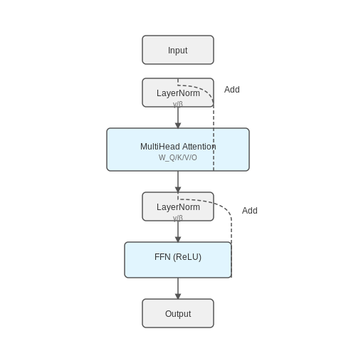
Before processing by either sub-layer, the input undergoes layer normalization, which stabilizes training by normalizing activations across the feature dimension. The normalized input is then passed through the sub-layer, and the result is added to the original input via a residual connection:

This residual connection ensures gradient flow during backpropagation, mitigating the vanishing gradient problem in deep networks. Layer normalization operates independently on each sequence element, computing statistics over the feature dimension:

where μ and σ² are the mean and variance of features, γ and β are learnable parameters, and ϵ is a small constant for numerical stability.

Multi-Head Self-Attention Mechanism

Each encoder layer employs multi-head self-attention to capture diverse relationships between input tokens. The input is projected into h separate sets of queries, keys, and values, allowing the model to attend to information from different representation subspaces. For each head i:

The outputs of all heads are concatenated and linearly projected:

where W_i^Q, W_i^K, W_i^V are learned projection matrices for head i, and W^O is the output projection matrix.

Position-wise Feed-Forward Networks

Following self-attention, each encoder layer applies a position-wise feed-forward network (FFN) to every token independently. The FFN consists of two linear transformations with a ReLU activation in between:

Despite operating identically on each position, the FFN introduces non-linearity and enables interactions between different dimensions of the representation space. The hidden layer typically has a larger dimensionality (e.g., 2048) than the input/output (e.g., 512), acting as a bottleneck that encourages information compression.

Stacking Encoder Layers

Multiple encoder layers are stacked to form a deep representation hierarchy. Lower layers capture local patterns and syntactic relationships, while higher layers model more abstract semantic features. The number of layers varies across architectures:

• Base Transformer: 6 encoder layers
• BERT-base: 12 encoder layers
• BERT-large: 24 encoder layers
• GPT-3: Up to 96 encoder-like layers (in decoder-only configuration)

As information propagates through the stack, gradient flow is maintained through residual connections, while layer normalization prevents exploding activations. The combination of self-attention and FFNs allows each layer to refine representations by incorporating both global context and localized feature transformations.

Decoder Stack: Masked Attention and Output Generation

Masked Multi-Head Attention Mechanism

The decoder's first sub-layer employs masked multi-head attention to ensure autoregressive properties during sequence generation. Unlike the encoder, which processes all tokens simultaneously, the decoder restricts attention to preceding tokens only. This is achieved by applying a causal mask to the attention scores before the softmax operation:

where i and j represent target and source positions, respectively. The masking ensures that during training, predictions for position i depend only on known outputs at positions less than i.

Mathematical Derivation of Masked Attention

Given input embeddings X ∈ ℝ^n×d, the masked attention computation proceeds as:

1. Project X into queries, keys, and values:
   $$ Q = XW_Q, \quad K = XW_K, \quad V = XW_V $$
2. Compute scaled dot-product attention scores:
   $$ A = \frac{QK^T}{\sqrt{d_k}} $$
3. Apply causal mask element-wise:
   $$ A_{masked} = A + M \quad \text{where } M_{ij} = \text{Mask}(i,j) $$
4. Compute softmax and weighted sum:
   $$ \text{Attention}(Q,K,V) = \text{softmax}(A_{masked})V $$

Encoder-Decoder Attention Layer

The second sub-layer performs cross-attention between decoder queries and encoder memory. The keys and values are derived from the encoder's output, while queries come from the previous decoder layer:

This allows each decoding step to dynamically attend to the most relevant parts of the input sequence, a critical feature for tasks like machine translation where alignment between source and target is non-monotonic.

Position-wise Feed-Forward Networks

Each decoder layer contains a position-wise FFN identical to the encoder's:

The FFN provides additional nonlinear transformations while maintaining positional independence, allowing each token to be processed separately after attention aggregation.

Output Generation Process

During inference, the decoder operates autoregressively:

• Step 1: Initialize with start token 〈sos〉
• Step 2: For each position i:
  1. Compute decoder states up to position i
  2. Generate logits via final linear projection:
     $$ z_i = h_iW_{vocab} $$
  3. Sample next token from distribution p_i = softmax(z_i)
• Termination: Repeat until end token 〈eos〉 is generated

Teacher Forcing During Training

When ground truth targets are available, training uses teacher forcing - feeding correct previous tokens regardless of model predictions. This is implemented by:

• Right-shifting the target sequence
• Using the shifted sequence as decoder input
• Computing loss against original targets

The parallel processing capability is maintained through masking, while still enforcing the autoregressive constraint.

Beam Search Decoding

For improved generation quality, inference often employs beam search:

where k maintains the top-B partial sequences at each step. Practical implementations include length normalization to prevent bias toward shorter outputs:

with α typically between 0.6 and 1.0.

4.1 Loss Functions: Cross-Entropy and Label Smoothing

Cross-Entropy Loss

The cross-entropy loss, also known as the negative log-likelihood loss, is the standard loss function for classification tasks in transformer models. Given a true probability distribution p and a predicted distribution q, the cross-entropy H(p, q) measures the dissimilarity between them:

In classification, p is a one-hot encoded vector where the true class has probability 1, and all others are 0. For a batch of N samples, the loss becomes:

where y_n is the true class for sample n, and q_n,yn is the predicted probability for that class. This formulation encourages the model to assign high confidence to the correct class.

Numerical Stability and Log-Space Computation

In practice, cross-entropy is computed in log-space to avoid numerical underflow when probabilities become extremely small. The softmax function is applied to model logits z before computing the loss:

This leads to the numerically stable implementation combining softmax and cross-entropy:

Label Smoothing

Standard cross-entropy with one-hot labels can lead to overconfidence, where models assign near-1 probabilities to the correct class. Label smoothing addresses this by replacing the one-hot labels with a mixture of the original distribution and a uniform distribution:

where α is the smoothing parameter (typically 0.1) and K is the number of classes. The smoothed cross-entropy loss becomes:

This regularization technique prevents the model from becoming overconfident and improves generalization, particularly in low-data regimes or when label noise is present.

Practical Considerations

Label smoothing introduces a trade-off between model confidence and calibration. While it improves robustness, excessive smoothing (α > 0.2) can degrade performance by making the targets too uniform. The optimal value depends on the dataset and task complexity.

In transformer architectures, label smoothing is commonly applied in machine translation and text classification tasks. For example, the original Transformer paper used α = 0.1 for WMT translation tasks, while BERT and GPT variants often use α = 0.0 or smaller values (α = 0.05) for language modeling.

4.2 Optimizers: Adam and Adaptive Learning Rates

The Limitations of Fixed Learning Rates

Traditional gradient descent optimizers like SGD use a fixed learning rate η for all parameters throughout training. This approach suffers from two key issues:

• Parameters with small gradients may converge too slowly.
• Parameters with large gradients may oscillate or diverge.

The learning rate dilemma becomes particularly acute in transformer architectures where attention weights and feed-forward layers exhibit vastly different gradient scales. Adaptive methods address this by maintaining parameter-specific learning rates.

Momentum and RMSProp Foundations

Adam combines two key ideas from earlier optimizers:

• Momentum (from Polyak, 1964): Accumulates an exponentially decaying average of past gradients to accelerate convergence.
• RMSProp (Hinton, 2012): Maintains a moving average of squared gradients to normalize the learning rate.

The momentum term helps navigate ravines (areas with steep curvature) while RMSProp adapts to gradient magnitudes.

Adam's Algorithmic Formulation

Adam maintains two state variables for each parameter θ_t at timestep t:

where g_t is the gradient, and β₁, β₂ ∈ [0,1) are decay rates (typically 0.9 and 0.999 respectively). The first moment m_t estimates the mean gradient while the second moment v_t estimates the uncentered variance.

Bias Correction

Since the moments are initialized at zero, they exhibit bias toward zero during early timesteps. Adam corrects this via:

The Complete Update Rule

The parameter update combines the corrected moments:

where ε (typically 10^-8) prevents division by zero. The denominator acts as an adaptive learning rate that:

• Decreases for parameters with large historical gradients
• Increases for parameters with small historical gradients

Practical Considerations in Transformers

When applied to transformer training:

• The attention layer gradients often exhibit sudden spikes due to softmax saturation
• Feed-forward network gradients tend to be more stable
• Adam's per-parameter adaptation helps stabilize attention layer updates while allowing sufficient movement in FFN weights

Empirical studies show Adam converges 2-3× faster than SGD with momentum on transformer language models while maintaining similar final performance.

Numerical Stability and Implementation

The square root and division in the update rule require careful numerical handling:

def adam_update(grad, m, v, t, lr=0.001, beta1=0.9, beta2=0.999, eps=1e-8):
    m = beta1 * m + (1 - beta1) * grad
    v = beta2 * v + (1 - beta2) * (grad  2)
    m_hat = m / (1 - beta1  t)
    v_hat = v / (1 - beta2 ** t)
    update = lr * m_hat / (np.sqrt(v_hat) + eps)
    return update, m, v
  

Variants and Improvements

Recent variants address observed limitations:

• AdamW: Decouples weight decay from gradient updates
• NAdam: Incorporates Nesterov momentum for smoother updates
• AMSGrad: Maintains the maximum of v_t to prevent convergence issues

4.3 Regularization Strategies: Dropout and Weight Decay

Regularization is critical in transformer models to prevent overfitting, especially given their large parameter counts. Two widely used techniques are dropout and weight decay, each addressing different aspects of model generalization.

Dropout in Transformers

Dropout randomly deactivates neurons during training with probability p, forcing the network to rely on distributed representations. In transformers, dropout is applied to:

• Attention weights: Dropout masks entries in the attention matrix before softmax normalization.
• Feed-forward layers: Randomly zeroes hidden units in position-wise MLPs.
• Residual connections: Applied to the output of sub-layers before adding to the residual stream.

The forward pass with dropout can be formalized for a given layer input x:

where m is a binary mask sampled from Bernoulli(1-p), and scaling by 1/(1-p) maintains activation magnitudes during training. At inference, dropout is disabled.

Weight Decay (L2 Regularization)

Weight decay adds a penalty term to the loss function proportional to the squared L2 norm of the parameters:

where λ controls regularization strength. This discourages large weight values without explicit constraints. In Adam-based optimizers, weight decay is decoupled from gradient updates (Loshchilov & Hutter, 2019):

where η is the learning rate, and m̂_t, v̂_t are bias-corrected momentum estimates.

Practical Considerations

Optimal dropout rates (p) and weight decay (λ) depend on model size and data:

• Large models: Typically use lower dropout (0.1–0.2) due to implicit regularization from overparameterization.
• Small datasets: Benefit from higher weight decay (0.01–0.1) to constrain capacity.
• Attention layers: Often apply higher dropout (0.2–0.3) than feed-forward layers (0.1–0.2).

Empirical studies show transformers are particularly sensitive to dropout placement—applying it to attention scores rather than value matrices yields better stability (Zhou et al., 2020).

Interaction with Other Components

Regularization interacts with key transformer mechanisms:

• Layer normalization: Dropout before normalization requires careful scaling to maintain variance.
• Residual connections: High dropout rates can disrupt gradient flow through deep networks.
• Warmup: Weight decay combined with learning rate warmup requires proportional λ adjustment.

5.1 BERT and GPT: Encoder-Only vs. Decoder-Only Models

Architectural Distinctions

The fundamental difference between BERT (Bidirectional Encoder Representations from Transformers) and GPT (Generative Pre-trained Transformer) lies in their architectural design. BERT employs an encoder-only Transformer stack, while GPT relies on a decoder-only structure. The encoder in BERT processes input tokens bidirectionally, allowing each token to attend to all other tokens in the sequence. In contrast, GPT's decoder uses masked self-attention, restricting each token to attend only to previous tokens in the sequence, making it inherently autoregressive.

For BERT, the attention mechanism computes pairwise interactions across all tokens, enabling rich contextual representations. GPT's masked attention ensures causality, critical for generative tasks:

where M is a lower-triangular mask matrix with −∞ in positions corresponding to future tokens.

Training Objectives

BERT is trained using a masked language modeling (MLM) objective, where randomly selected tokens are masked, and the model predicts them based on bidirectional context. Additionally, BERT employs next sentence prediction (NSP) to learn relationships between sentences. GPT, however, is trained purely via autoregressive language modeling, predicting each token conditioned on preceding tokens, maximizing the likelihood:

5.2 Efficient Transformers: Sparse Attention and Memory Optimization

Attention Sparsity and Computational Complexity

Locality-Sensitive Hashing (LSH) Attention

Block-Sparse Attention Patterns

• Local windows: Each token attends to a fixed neighborhood (e.g., 256 preceding tokens)
• Global tokens: Selected tokens attend to all positions (e.g., CLS token in BERT)
• Random connections: Each token attends to a random subset of distant positions

Memory-Efficient Attention Computation

1. Gradient checkpointing: Recomputes attention activations during backward pass rather than storing them
2. Memory-efficient kernels: Fused attention operations that avoid materializing the full n×n matrix

• Tiling attention computation to fit in SRAM
• Fusing softmax operations with backward pass
• Maintaining exact attention computation (no approximation)

Low-Rank and Kernel Approximations

5.3 Cross-Attention Mechanisms in Multimodal Models

Cross-attention mechanisms enable transformers to process and align information across different modalities, such as text, images, and audio. Unlike self-attention, which operates within a single modality, cross-attention computes interactions between two distinct sequences—typically a query sequence from one modality and key-value pairs from another.

Mathematical Formulation

Given a query sequence Q from modality A and key-value pairs K, V from modality B, cross-attention computes:

Where d_k is the dimension of the key vectors. The softmax operation ensures that the attention weights sum to one, allowing the model to focus on relevant parts of the input sequence.

Architectural Implementation

In multimodal transformers like Vision-Language Pretraining (VLP) models, cross-attention layers are interleaved with self-attention layers. For example:

• Encoder-Decoder Models: The decoder uses cross-attention to attend to the encoder's output (e.g., text-to-image generation in DALL·E).
• Fusion Architectures: Models like CLIP employ cross-attention to align visual and textual embeddings in a shared latent space.

Practical Applications

Cross-attention is pivotal in tasks requiring modality alignment:

• Image Captioning: The decoder attends to visual features extracted by a CNN or ViT encoder.
• Multimodal Translation: Speech-to-text models use cross-attention to map audio spectrograms to text tokens.
• Document Understanding: LayoutLM combines text and spatial coordinates via cross-attention.

Challenges and Optimizations

Cross-modal attention introduces computational and optimization challenges:

• Modality Gap: Features from different modalities may reside in disjoint embedding spaces. Techniques like contrastive learning (e.g., in ALIGN) mitigate this by pulling aligned pairs closer in the latent space.
• Scalability: Processing long sequences (e.g., high-resolution images) requires approximations like perceiver architectures or sparse attention.

Case Study: Flamingo (DeepMind)

Flamingo integrates cross-attention between frozen vision encoders (e.g., NFNet) and a pretrained language model (e.g., Chinchilla). The model processes interleaved image-text sequences by:

1. Projecting visual features into the text token space.
2. Applying cross-attention in the language model's decoder layers.

Where W_Q, W_K, and W_V are learned projection matrices.

Natural Language Processing: Translation and Summarization

Transformer-Based Translation

Sequence-to-Sequence Learning in Transformers

6.2 Computer Vision: Vision Transformers (ViTs)

Architectural Adaptation of Transformers for Images

Vision Transformers (ViTs) adapt the transformer architecture—originally designed for sequential data—to handle 2D image data. The key challenge lies in converting spatially structured images into a sequence of tokens compatible with the transformer's self-attention mechanism. Unlike convolutional neural networks (CNNs), which inherently capture local spatial hierarchies, ViTs rely on global attention to model relationships between patches of an image.

Patch Embedding and Positional Encoding

Each patch 𝐱_p is linearly projected into a D-dimensional embedding space using a trainable matrix E ∈ ℝ^P²×C×D. To retain spatial information, learnable positional embeddings E_pos ∈ ℝ^N×D are added to the patch embeddings:

Unlike NLP transformers, ViTs often use 2D-aware positional encodings to preserve spatial relationships. Some variants employ sinusoidal encodings or relative position biases to enhance translation invariance.

Transformer Encoder for Vision

The core of a ViT consists of L identical transformer encoder layers. Each layer applies multi-head self-attention (MSA) and a feed-forward network (FFN) with layer normalization (LN) and residual connections:

The attention mechanism computes pairwise interactions between all patches, enabling global receptive fields from the first layer. This contrasts with CNNs, where receptive fields expand gradually with depth.

Hybrid Architectures and Efficiency

To mitigate ViTs' high computational cost (O(N²) in self-attention), hybrid models combine CNN feature maps with transformer layers. For example, ResNet-50 can generate lower-resolution patch embeddings before applying attention. Other optimizations include:

• Hierarchical Transformers (e.g., Swin Transformer): Local window attention with shifted windows reduces complexity to O(N).
• Linear Attention: Approximates softmax attention with kernel methods to achieve O(N) scaling.
• Patch Merging: Progressive downsampling of token sequences mimics CNN pooling.

Practical Applications and Performance

ViTs excel in tasks requiring long-range dependencies, such as:

• Image Classification: ViT-B/16 achieves 88.55% top-1 accuracy on ImageNet, surpassing ResNet-152 with fewer FLOPs.
• Object Detection: DETR (Detection Transformer) replaces handcrafted anchors with set prediction via transformers.
• Medical Imaging: ViTs outperform CNNs in segmenting irregular structures (e.g., tumors) due to global context modeling.

Challenges and Ongoing Research

ViTs face limitations in data efficiency, requiring large-scale pretraining (e.g., JFT-300M) to match CNNs trained on ImageNet alone. Recent advances address this via:

• Self-Supervised Pretraining (e.g., MAE, BeiT): Masked autoencoding of patches improves sample efficiency.
• Neural Architecture Search: Automates ViT configuration for specific hardware constraints.
• Dynamic Token Sparsification: Prunes less informative patches during inference to reduce compute.

6.3 Speech and Audio Processing: Transformer-Based ASR

Transformer Adaptation for Automatic Speech Recognition

Traditional automatic speech recognition (ASR) systems relied on hybrid architectures combining convolutional neural networks (CNNs), recurrent neural networks (RNNs), and hidden Markov models (HMMs). Transformers, with their self-attention mechanisms, have revolutionized ASR by enabling direct modeling of long-range dependencies in speech signals without sequential processing constraints. The key adaptation involves:

• Input Representation: Raw audio waveforms or log-mel spectrograms are processed using convolutional layers to generate frame-level embeddings before feeding into the transformer.
• Positional Encoding: Since speech is a time-series, sinusoidal or learned positional encodings are critical to preserve temporal order.
• Downsampling: Strided convolutions or pooling reduce sequence length to mitigate computational overhead from long audio inputs.

Self-Attention in Speech Contexts

The self-attention mechanism in transformers computes pairwise relationships between all frames in the input sequence. For an input sequence X ∈ ℝ^T×d (where T is the number of frames and d is the feature dimension), the attention weights A are computed as:

where Q, K, and V are learned linear projections of X. In speech, this allows the model to attend to phonetically relevant contexts (e.g., coarticulation effects) across arbitrary distances.

Architectural Variants for ASR

Conformer Architecture

The Conformer (Convolution-augmented Transformer) integrates convolutional layers within the transformer block to capture both local and global patterns. Each Conformer block consists of:

1. Multi-headed self-attention (MHSA) layer
2. Depthwise convolutional layer with kernel size k
3. Feed-forward network (FFN) with residual connections

Streamable Transformers

For real-time ASR, restricted self-attention variants like chunk-based attention or memory-compressed attention limit the context window to future frames, enabling low-latency streaming.

Training Paradigms

Modern transformer-based ASR systems often employ multi-task learning:

• Connectionist Temporal Classification (CTC): Provides frame-level alignment supervision.
• Attention-based Decoder: Autoregressively predicts tokens using cross-attention over encoder states.
• Self-Supervised Pretraining: Models like wav2vec 2.0 use contrastive learning on unlabeled audio before fine-tuning on transcribed data.

Performance Considerations

Transformer ASR models achieve state-of-the-art results on benchmarks like LibriSpeech, but face challenges:

• Compute Requirements: Quadratic attention complexity for long sequences necessitates optimizations like linear attention or locality-sensitive hashing.
• Data Efficiency: Transformers typically require more labeled data than RNNs, mitigated by self-supervised pretraining.
• Robustness: Performance degrades under acoustic noise, addressed through adversarial training or adaptive feature normalization.

Case Study: Whisper Architecture

OpenAI's Whisper model demonstrates transformer scalability for multilingual ASR:

• Processes raw audio via 80-channel log-mel spectrogram with 25ms windows
• Uses a 12-layer encoder with 768-dimensional embeddings and 12 attention heads
• Decoder autoregressively predicts text tokens with cross-attention over encoder outputs
• Trained on 680,000 hours of multilingual supervised data

7.1 Foundational Papers and Key Research

• Architecture and Working of Transformers in Deep Learning — Transformers are a type of deep learning model that utilizes self-attention mechanisms to process and generate sequences of data efficiently. They capture long-range dependencies and contextual relationships making them highly effective for tasks like language modeling, machine translation and text generation. In this article we will explore the architecture and working of transformers by ...
• From Turing to Transformers: A Comprehensive Review and Tutorial ... - MDPI — In recent years, generative transformers have become increasingly prevalent in the field of artificial intelligence, especially within the scope of natural language processing. This paper provides a comprehensive overview of these models, beginning with the foundational theories introduced by Alan Turing and extending to contemporary generative transformer architectures. The manuscript serves ...
• 11. Attention Mechanisms and Transformers — Dive into Deep ... - D2L — 11. Attention Mechanisms and Transformers The earliest years of the deep learning boom were driven primarily by results produced using the multilayer perceptron, convolutional network, and recurrent network architectures. Remarkably, the model architectures that underpinned many of deep learning's breakthroughs in the 2010s had changed remarkably little relative to their antecedents despite ...
• Transformer (deep learning architecture) - Wikipedia — A standard Transformer architecture, showing on the left an encoder, and on the right a decoder. Note: it uses the pre-LN convention, which is different from the post-LN convention used in the original 2017 Transformer. The transformer is a deep learning architecture that was developed by researchers at Google and is based on the multi-head attention mechanism, which was proposed in the 2017 ...
• [Part 2/20] Decoding the Architecture of Transformers: A ... - Medium — Image by AI Table of Contents 1. Understanding Transformer Architecture 2. Key Components of Transformers 2.1. Attention Mechanisms Explained 2.2. Positional Encoding and Its Role 3. Practical ...
• PDF CHAPTER The Transformer - Stanford University — The transformer is a neural network with a specific structure that includes a mechanism called self-attention or multi-head attention.1 Attention can be thought of as a way to build contextual representations of a token's meaning by attending to and integrating information from surrounding tokens, helping the model learn how tokens relate to each other over large spans.
• LLM Architectures Explained: Transformers (Part 6) - Medium — Deep Dive into the architecture & building real-world applications leveraging NLP Models starting from RNN to Transformer.
• PDF How Many Layers and Why? An Analysis of the Model Depth in Transformers — dynamic layers depth at the token level for full transformers (encoder-decoder). However, to the best of our knowledge, our attempt is the first to ap-ply such mechanism to encoder only transformers and to provide an analysis of the process.
• Transformer models: an introduction and catalog - arXiv.org — It is beyond the scope of this paper to go into all the details of the Transformer architecture. For that, we will refer you to the original paper ( ?) or to The Illustrated Transformer 3 post.
• PDF Transformers_S24 - Deep Learning — • Transformers seem to provide a new class of generalist models that are capable of capturing knowledge which is more fundamental than task-specific abilities.

7.2 Books and Comprehensive Guides

• 11.7. The Transformer Architecture — Dive into Deep Learning 1. ... - D2L — 11.7.1. Model As an instance of the encoder-decoder architecture, the overall architecture of the Transformer is presented in Fig. 11.7.1. As we can see, the Transformer is composed of an encoder and a decoder. In contrast to Bahdanau attention for sequence-to-sequence learning in Fig. 11.4.2, the input (source) and output (target) sequence embeddings are added with positional encoding ...
• Transformers and Inductors for Power Electronics Transformers and ... — The power supply remains one of the biggest components in portable electronic equipment. Power electronics is an enabling technology for power conversion in energy sys-tems. All power electronic converters have magnetic components in the form of transformers for power transfer and inductors for energy storage.
• 11. Attention Mechanisms and Transformers — Dive into Deep ... - D2L — 11. Attention Mechanisms and Transformers The earliest years of the deep learning boom were driven primarily by results produced using the multilayer perceptron, convolutional network, and recurrent network architectures. Remarkably, the model architectures that underpinned many of deep learning's breakthroughs in the 2010s had changed remarkably little relative to their antecedents despite ...
• Transformers for Machine Learning: A Deep Dive — 60+ transformer architectures covered in a comprehensive manner. A book for understanding how to apply the transformer techniques in speech, text, time series, and computer vision. Practical tips and tricks for each architecture and how to use it in the real world.
• Transformers and Inductors for Power Electronics: Theory, Design and ... — Covering the basics of the magnetic components of power electronic converters, this book is a comprehensive reference for students and professional engineers dealing with specialised inductor and transformer design.
• Transformer Engineering, 2nd Edition [Book] - O'Reilly Media — Transformers are one of the most critical components of power systems, and engineers need deep, practical knowledge about their design and operation. Blending theory and practice, this second edition of … - Selection from Transformer Engineering, 2nd Edition [Book]
• PDF 6.013 Electromagnetics and Applications, Course Notes — To meet the increasing educational challenge of providing both breadth and depth in electromagnetics within a brief presentation, this text uses a more physics-based approach and novel methods of explaining certain phenomena.
• PDF Principles of Power Electronics — Substantially expanded and updated, the new edition of this classic textbook provides unrivaled coverage of the fundamentals of power electronics. It includes: Comprehensive and up-to-date coverage of foundational concepts in circuits, mag-netics, devices, dynamic models, and control, establishing a strong conceptual frame-work for further study.
• Electronics/Transformer Design - Wikibooks, open books for an open world — The designer first needs several known factors to design a transformer. For a transformer using a sine or square wave, one needs to know the incoming line voltage, the operating frequency, the secondary voltage (s), the secondary current (s), the permissible temperature rise, the target efficiency, the physical size one can use, and the cost limitations. Once these factors are known, design ...
• PDF Basic Electrical Engineering By Fitzerald — The design of transformers, functioning of generators and performance of induction motors are explained through descriptive illustrations, step-by-step solved examples and mathematical derivations.

7.3 Online Courses and Tutorials

• Transformer Architectures | SpringerLink — Transformers, with their extensive pre-training on large corpora and flexible architecture, are particularly well-suited for transfer learning. This section explores the principles of transfer learning with transformers, focusing on pre-training and fine-tuning, as well as domain adaptation.
• 11.7. The Transformer Architecture — Dive into Deep Learning 1. ... - D2L — 11.7.1. Model As an instance of the encoder-decoder architecture, the overall architecture of the Transformer is presented in Fig. 11.7.1. As we can see, the Transformer is composed of an encoder and a decoder. In contrast to Bahdanau attention for sequence-to-sequence learning in Fig. 11.4.2, the input (source) and output (target) sequence embeddings are added with positional encoding ...
• D2L - Dive into Deep Learning — Dive into Deep Learning 1.0.3 ... — New topics of reinforcement learning, Gaussian processes, and hyperparameter optimization are added! [Jul 2022] Check out our new API for implementation and new topics like generalization in classification and deep learning, ResNeXt, CNN design space, and transformers for vision and large-scale pretraining.
• Computation Structures | Electrical Engineering and Computer Science ... — This course introduces architecture of digital systems, emphasizing structural principles common to a wide range of technologies. It covers the topics including multilevel implementation strategies, definition of new primitives (e.g., gates, instructions, procedures, processes) and their mechanization using lower-level elements. It also includes analysis of potential concurrency, precedence ...
• Transformer (deep learning architecture) - Wikipedia — A standard Transformer architecture, showing on the left an encoder, and on the right a decoder. Note: it uses the pre-LN convention, which is different from the post-LN convention used in the original 2017 Transformer. The transformer is a deep learning architecture that was developed by researchers at Google and is based on the multi-head attention mechanism, which was proposed in the 2017 ...
• PDF Introduction to Electrical Computer Science and Engineering — This material is intended for the first course sequence in Electrical Engineering focused on Electrical Circuit Analysis and Design. The content is derived from the author's educational, engineering and management career, and teaching experience.
• 23.7 Transformers - College Physics — Transformers do what their name implies—they transform voltages from one value to another (The term voltage is used rather than emf, because transformers have internal resistance). For example, many cell phones, laptops, video games, and power tools and small appliances have a transformer built into their plug-in unit (like that in Figure 1) that changes 120 V or 240 V AC into whatever ...
• 42.130. Complete the transformer architecture — Ocademy Open Machine ... — 42.130.1. Transformer Model The encoder-decoder architecture based on the Transformer structure is illustrated in figure below. The left and right sides correspond to the encoder and decoder structures, respectively. They consist of several basic Transformer blocks (represented by the gray boxes in the figure), stacked N times. Each component comprises multiple Transformer blocks, which are ...
• Introduction to Electronics - Coursera — Offered by Georgia Institute of Technology. This course introduces students to the basic components of electronics: diodes, transistors, and ... Enroll for free.
• PDF Lecture Notes for Analog Electronics - University of Oregon — Lecture Notes for Analog Electronics Raymond E. Frey Physics Department University of Oregon Eugene, OR 97403, USA [email protected]