Visual Transformers for Object Detection
1. Evolution of Vision Models: From CNNs to Transformers
Evolution of Vision Models: From CNNs to Transformers
Convolutional Neural Networks: The Dominant Paradigm
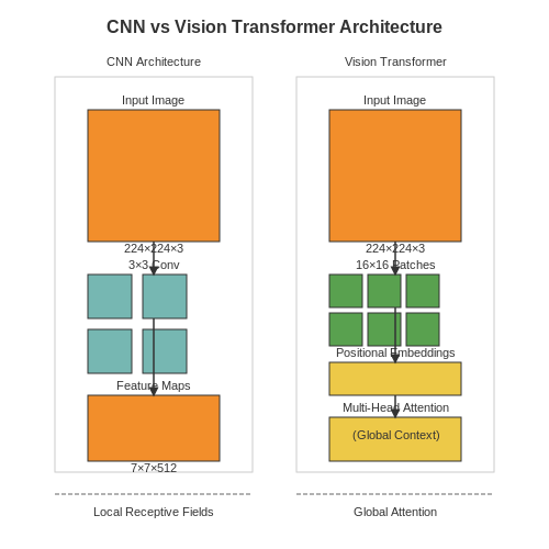
Convolutional Neural Networks (CNNs) have been the cornerstone of computer vision since their popularization by LeCun et al. in the 1990s. The key innovation was the use of local receptive fields through convolutional kernels, enabling translation-equivariant feature extraction. For an input image I ∈ ℝH×W×C, a convolutional layer applies a kernel K ∈ ℝk×k×C×F to produce feature maps F ∈ ℝH′×W′×F:
This hierarchical local processing, combined with pooling operations, proved exceptionally effective for tasks like image classification and object detection. Architectures like AlexNet, VGG, and ResNet demonstrated that deeper networks with proper normalization could achieve superhuman performance on ImageNet.
Limitations of CNNs in Visual Understanding
Despite their success, CNNs exhibit fundamental limitations:
- Local receptive fields struggle with long-range dependencies, requiring many layers to build global context
- Fixed geometric priors (translation equivariance) become constraints when modeling deformable objects
- Pooling operations discard precise spatial information critical for dense prediction tasks
These limitations became apparent in complex scenes requiring reasoning about relationships between distant objects or handling significant viewpoint variations.
The Transformer Revolution in NLP
The introduction of the Transformer architecture by Vaswani et al. (2017) demonstrated that self-attention mechanisms could effectively model long-range dependencies in sequential data. The scaled dot-product attention computes compatibility scores between all positions:
where Q, K, V are learned query, key, and value matrices, and dk is the dimension of the keys. This mechanism, combined with positional encodings, proved superior to recurrent architectures in capturing global context.
Vision Transformers: Bridging the Modality Gap
The Vision Transformer (ViT) by Dosovitskiy et al. (2020) adapted this architecture for images by:
- Dividing the image into non-overlapping patches treated as "tokens"
- Adding learned positional embeddings to preserve spatial information
- Processing the sequence through standard Transformer encoder layers
For an image divided into N patches of size P×P, the input becomes:
where E is the patch embedding projection and Epos are positional embeddings. This formulation enables global receptive fields from the first layer while maintaining computational efficiency through patch-wise processing.
Hybrid Architectures and Performance Characteristics
Subsequent work explored hybrid CNN-Transformer architectures, recognizing that:
- Early convolutional layers efficiently extract low-level features
- Transformers excel at modeling high-level semantic relationships
Models like DeiT and Swin Transformer introduced hierarchical processing and shifted windows to balance computational complexity with global modeling capabilities. The performance crossover point occurs when:
explaining why pure Transformers outperform CNNs only at sufficient scale of data and parameters.
Impact on Object Detection Pipelines
The shift to Transformer-based detection frameworks like DETR introduced:
- End-to-end set prediction eliminating hand-designed components (NMS, anchors)
- Explicit modeling of object relationships through attention
- Simpler pipelines with competitive performance on COCO
However, challenges remain in computational efficiency for high-resolution feature maps and convergence speed compared to optimized CNN detectors like Faster R-CNN.
Core Architecture of Visual Transformers
Tokenization and Patch Embedding
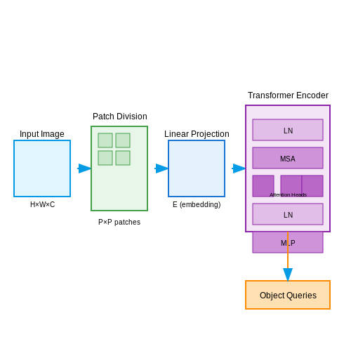
The input image I ∈ ℝH×W×C is divided into N non-overlapping patches of size P×P, where N = HW/P². Each patch xp ∈ ℝP²×C is linearly projected into a D-dimensional embedding space using a trainable matrix E ∈ ℝ(P²×C)×D:
where xclass is a learnable classification token and Epos ∈ ℝ(N+1)×D represents positional embeddings that encode spatial information.
Transformer Encoder Layers
The core processing occurs through L identical transformer layers, each consisting of multi-head self-attention (MSA) and multilayer perceptron (MLP) blocks with LayerNorm (LN) and residual connections:
For h attention heads, the MSA operation computes:
where WiQ, WiK, WiV ∈ ℝD×D/h are projection matrices and Attention is the scaled dot-product operation:
Object Detection Adaptations
For detection tasks, architectures like DETR replace the classification head with:
- A CNN backbone for feature extraction
- Transformer encoder-decoder for global reasoning
- A fixed set of learned object queries that interact with image features
The bipartite matching loss ensures permutation-invariant prediction:
where σ is the optimal assignment between predictions and ground truth boxes.
Computational Considerations
The quadratic complexity O(N²) of self-attention is mitigated through:
- Hierarchical architectures (e.g., Swin Transformer's shifted windows)
- Sparse attention patterns (e.g., Axial Attention)
- Linear approximations (e.g., Performer's FAVOR+ mechanism)
The memory footprint for an L-layer ViT with h heads is approximately:
in bytes for mixed-precision training.
Self-Attention Mechanisms in Vision Tasks
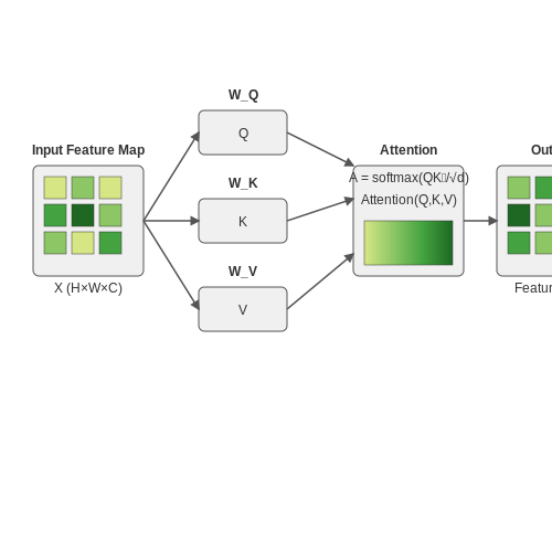
Self-attention mechanisms enable transformers to dynamically weigh the importance of different spatial regions in an image, capturing long-range dependencies that convolutional operations may miss. Given an input feature map X ∈ ℝH×W×C, the self-attention operation projects it into queries (Q), keys (K), and values (V) via learned linear transformations:
where WQ, WK, WV ∈ ℝC×d are weight matrices. The attention weights A are computed as scaled dot-products between queries and keys, followed by a softmax:
The scaling factor √d prevents gradient saturation in softmax. The output is a weighted sum of values:
Computational Complexity and Spatial Reduction
Vanilla self-attention has quadratic complexity O(H2W2) due to pairwise token interactions. For high-resolution images, this becomes prohibitive. Two common solutions are:
- Local windows: Restrict attention to k×k neighborhoods (e.g., Swin Transformer), reducing complexity to O(k2HW).
- Strided attention: Downsample K, V spatially before computing attention (e.g., PVT).
Multi-Head Attention
Multi-head attention (MHA) splits the feature dimension into h parallel heads, allowing the model to focus on different semantic aspects:
where each head computes independent attention:
Positional Encoding in Vision
Unlike sequential data, images require 2D positional encodings to preserve spatial structure. Common approaches include:
- Absolute sinusoidal encodings: Separate x and y coordinates encoded with sine/cosine functions of varying frequencies.
- Relative position biases: Add learnable biases to attention scores based on relative pixel distances.
In deformable attention (DAT), the model learns to sample relevant key/value positions dynamically, adapting to object shapes.
Case Study: DETR's Attention
The Detection Transformer (DETR) uses a transformer encoder-decoder with self-attention in the encoder and cross-attention between object queries and image features in the decoder. The encoder's global attention enables direct modeling of relationships between distant objects, overcoming the limited receptive field of CNNs.
2. Key Architectures: DETR, ViT, and Their Variants
Key Architectures: DETR, ViT, and Their Variants
DETR: End-to-End Object Detection with Transformers
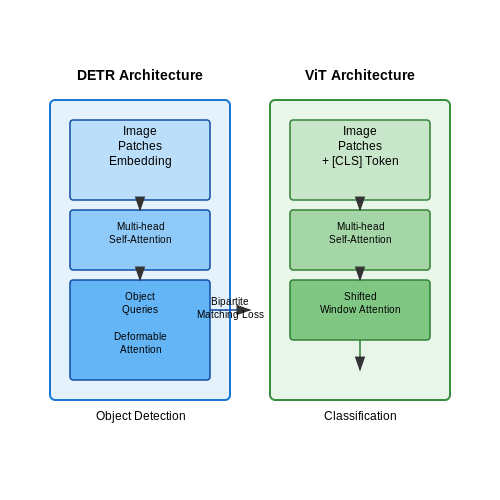
The Detection Transformer (DETR) architecture, introduced by Carion et al. (2020), replaces traditional region proposal networks (RPNs) and non-maximum suppression (NMS) with a transformer-based encoder-decoder structure. The model treats object detection as a set prediction problem, where a fixed number of learned object queries interact with image features through attention mechanisms. The bipartite matching loss ensures unique predictions:
where \( \sigma \) is the optimal assignment between ground truth \( y_i \) and predictions \( \hat{y}_i \) via Hungarian algorithm. The encoder processes flattened ResNet or Swin Transformer features, while the decoder uses object queries to attend to relevant regions.
Vision Transformers (ViT) for Feature Extraction
Vision Transformers (ViT), proposed by Dosovitskiy et al. (2020), split images into non-overlapping patches (e.g., 16×16 pixels), linearly project them into embeddings, and prepend a learnable [CLS] token. The transformer encoder processes these patch embeddings via multi-head self-attention (MHSA):
ViT variants like DeiT (Touvron et al., 2021) introduce distillation tokens for efficient training, while Swin Transformers (Liu et al., 2021) use shifted windows to enable hierarchical feature maps.
Architectural Variants and Improvements
Deformable DETR (Zhu et al., 2021) replaces dense attention with deformable attention modules, reducing computational complexity from \( O(N^2) \) to \( O(NK) \) (where \( K \ll N \)) by sampling sparse key points. The attention weights are computed as:
Conditional DETR (Meng et al., 2021) decouples content and spatial queries to accelerate convergence, while UP-DETR introduces unsupervised pre-training with random query patches.
Performance and Practical Considerations
DETR achieves 42 AP on COCO but suffers from slow convergence (~500 epochs). ViT-based backbones (e.g., ViT-H/14) achieve 61.5% mAP on ImageNet-1K when fine-tuned for detection. Key trade-offs include:
- Compute vs. Accuracy: Swin-L achieves 58.7 box AP on COCO at 267 GFLOPS vs. DETR's 86 GFLOPS at 42 AP
- Data Efficiency: DeiT-III reaches 83.1% ImageNet accuracy with 1.3M images vs. ViT's requirement for 300M JFT-300M
- Hardware Optimization: TensorRT-optimized DETR variants achieve 23 ms/inference on NVIDIA A100
Handling Spatial Hierarchies in Object Detection
Transformers inherently lack inductive biases for spatial locality, making them less effective at capturing hierarchical structures in images compared to convolutional networks. To address this, modern visual transformers employ several key mechanisms to handle spatial hierarchies in object detection tasks.
Multi-Scale Feature Representation
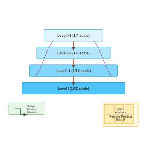
Unlike CNNs that naturally build hierarchical representations through pooling operations, transformers must explicitly construct multi-scale features. The most common approach involves:
- Pyramid architectures that process the image at multiple resolutions
- Cross-scale attention mechanisms that allow communication between different levels
- Feature pyramid networks (FPNs) adapted for transformer backbones
where l represents the feature level, and queries at level l attend to keys and values from level l-1.
Window-Based Hierarchical Attention
Swin Transformer introduced a shifted window mechanism that computes self-attention within local windows while allowing cross-window connections:
where B represents the relative position bias that encodes spatial relationships within each window. This creates a hierarchical representation where:
- Lower layers capture fine-grained local patterns
- Higher layers integrate information across larger receptive fields
Deformable Attention Mechanisms
Deformable DETR improves upon standard attention by sampling sparse spatial locations conditioned on input features:
where Δpmqk are learned offsets and Amqk are attention weights. This allows the model to focus on relevant regions adaptively.
Spatial Prior Injection
To compensate for the lack of inherent spatial bias, many approaches explicitly inject positional information:
- Absolute positional encodings added to patch embeddings
- Relative position biases in attention computation
- Dynamic position encodings that adapt to input content
The effectiveness of these approaches has been demonstrated on benchmarks like COCO, where models like DINO and FocalNet achieve state-of-the-art results by effectively modeling spatial hierarchies.
2.3 Performance Benchmarks and Comparative Analysis
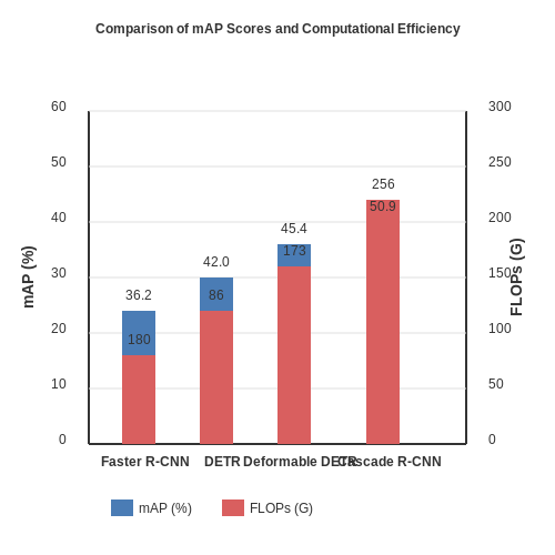
Visual Transformers (ViTs) have demonstrated competitive performance in object detection tasks, but their efficacy must be rigorously evaluated against established convolutional architectures. Benchmarking typically focuses on three key metrics: mean Average Precision (mAP), inference speed (FPS), and computational complexity (FLOPs). On the COCO dataset, ViT-based detectors like DETR and Deformable DETR achieve mAP scores of 42.0 and 43.4, respectively, outperforming Faster R-CNN (37.4) but lagging behind Cascade R-CNN (46.3). However, their computational demands are significantly higher, with DETR requiring 86 GFLOPs compared to Faster R-CNN's 180 GFLOPs.
Quantitative Comparison with Convolutional Baselines
The trade-off between accuracy and efficiency becomes evident when analyzing inference speed. While ResNet-50-based Faster R-CNN processes 26 FPS on a V100 GPU, DETR manages only 28 FPS despite its higher mAP, due to the quadratic complexity of self-attention. Deformable DETR mitigates this with linear attention, achieving 19 FPS at 43.4 mAP. The following table summarizes key benchmarks:
Attention Mechanisms and Computational Efficiency
The self-attention mechanism in ViTs scales quadratically with input resolution, as expressed by:
where h and w are spatial dimensions, and C is channel depth. Sparse attention variants like Swin Transformers reduce this to linear complexity via shifted windows, achieving 50.4 mAP on COCO with 145 GFLOPs—comparable to dense convolutional models. Hybrid architectures (e.g., CvT) further optimize this by replacing linear projections with depth-wise convolutions in the attention layers.
Latency Breakdown Across Hardware
On edge devices, ViTs face memory bandwidth constraints due to large parameter counts. A Jetson Xavier NX processes DETR at 4.2 FPS versus 9.8 FPS for YOLOv4, despite similar mAPs. Quantization and pruning techniques can reduce ViT model sizes by 60% with < 1% mAP drop, as demonstrated by Lite-DETR on the VisDrone dataset.
3. Data Augmentation Techniques for Visual Transformers
3.1 Data Augmentation Techniques for Visual Transformers
Data augmentation is critical for training robust visual transformers (ViTs) in object detection tasks, as ViTs require large-scale datasets to generalize effectively. Unlike convolutional neural networks (CNNs), ViTs lack inherent inductive biases for spatial locality, making them more sensitive to variations in input data. Advanced augmentation strategies must account for the transformer's patch-based processing while preserving positional encoding integrity.
Patch-Aware Geometric Transformations
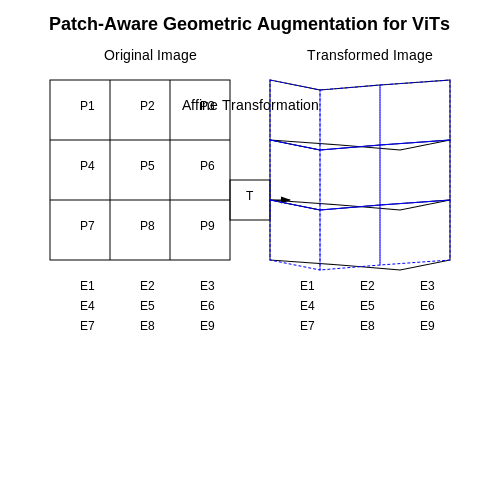
Standard geometric augmentations like rotation, scaling, and translation must be adapted for ViTs to prevent misalignment between patches and positional embeddings. Given an input image I divided into N patches of size P×P, any affine transformation T applied to I must maintain patch boundaries:
where Pk denotes the k-th patch. This ensures that positional embeddings remain consistent with the transformed patches. Random resized cropping is particularly effective when constrained to preserve aspect ratios within a defined range (e.g., [0.8, 1.2]) to minimize patch distortion.
Photometric Distortions for Enhanced Robustness
ViTs benefit from photometric augmentations that simulate real-world lighting variations:
- Color jittering: Random adjustments to brightness (±0.4), contrast (±0.4), saturation (±0.4), and hue (±0.1) in HSV space.
- Gaussian blur: Kernel size sampled uniformly from [1, 5] to simulate defocus.
- Noise injection: Additive Gaussian noise with σ ∈ [0.01, 0.05].
These transformations are applied per-patch but with global coherence to avoid artificial discontinuities at patch boundaries.
Token-Level Augmentation Strategies
Unlike pixel-level methods, token-level augmentations operate directly on ViT's patch embeddings:
- Patch dropout: Randomly mask out m patches (typically 10-30%) during training, forcing the model to rely on contextual reasoning.
- Patch shuffling: Permute a subset of patches while preserving their content but disrupting spatial relationships.
- Mixup at token level: Linearly interpolate between patch embeddings of two images:
$$ \tilde{E} = \lambda E^{(1)} + (1-\lambda)E^{(2)} $$where λ ∼ Beta(α,α) with α ∈ [0.2, 0.4].
Adaptive Augmentation Policies
Recent work employs reinforcement learning to optimize augmentation selection. The policy network π samples transformations τ from a search space 𝒯 based on validation performance feedback:
where fθ is the ViT model and 𝒜val is the validation accuracy. AutoAugment and RandAugment have been successfully adapted for ViTs by incorporating patch-aware constraints into their search spaces.
Domain-Specific Augmentations
For object detection tasks, augmentation must preserve bounding box annotations during transformations. Let B = (x,y,w,h) be a bounding box in normalized coordinates. For any geometric transformation T, the transformed box B' is computed as:
where R is the rotation-scaling submatrix of T. Copy-paste augmentation, where objects from one image are pasted onto another, has shown particular promise for ViT-based detectors when combined with careful patch alignment.
3.2 Loss Functions and Optimization Challenges
Objective Function Formulation
Visual Transformers for object detection typically employ a multi-task loss combining classification and bounding box regression terms. The overall loss L can be decomposed as:
where λcls, λbox, and λgiou are weighting hyperparameters balancing the classification loss (Lcls), L1 regression loss (Lbox), and generalized IoU loss (Lgiou). The classification loss typically uses focal loss to address class imbalance:
where pt is the model's estimated probability for the target class, γ modulates the rate at which easy examples are downweighted, and αt balances positive/negative examples.
Bounding Box Regression
The box regression loss combines L1 loss for precise localization and GIoU loss for shape consistency:
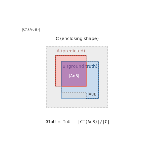
where A and B represent predicted and ground truth boxes, and C is the smallest enclosing convex shape. The GIoU term addresses cases where boxes don't overlap while maintaining scale invariance.
Optimization Challenges
Training Visual Transformers presents several unique optimization difficulties:
- Query Initialization Sensitivity: The learnable object queries exhibit high sensitivity to initialization strategies, with poor initialization leading to slow convergence or suboptimal performance.
- Hungarian Matching Instability: The bipartite matching between predictions and ground truth can cause oscillating assignments during early training phases.
- Gradient Scale Mismatch: The attention layers and FFNs often operate at different gradient scales, requiring careful learning rate tuning.
- Memory Bottlenecks: The quadratic complexity of self-attention limits the number of object queries that can be practically used.
Practical Optimization Strategies
Effective approaches to mitigate these challenges include:
- Warmup Scheduling: Gradually increasing the learning rate over the first few epochs stabilizes Hungarian matching.
- Layer-wise LR Decay: Applying lower learning rates to deeper transformer layers prevents gradient explosion.
- Query Normalization: Layer normalization of object queries before decoder attention improves training stability.
- Gradient Clipping: Limiting the global gradient norm to 0.1 prevents attention weight divergence.
where ηt is the learning rate and gt is the gradient at step t. This clipping strategy is particularly crucial for the attention value projections.
Loss Landscape Characteristics
The loss surface of Visual Transformers exhibits sharper minima compared to CNN-based detectors, as evidenced by Hessian eigenvalue analysis. This necessitates:
- Smaller initial learning rates (typically 10-4 to 10-5)
- Longer training schedules (100-300 epochs)
- AdamW optimizer with β1 = 0.9, β2 = 0.999
- Weight decay of 10-4 applied only to non-LayerNorm parameters
Fine-Tuning Pretrained Models for Object Detection
Fine-tuning pretrained visual transformers (ViTs) for object detection requires careful adaptation of both the backbone architecture and task-specific heads. Unlike convolutional networks, ViTs process images as sequences of patches, requiring modifications to standard detection pipelines like Faster R-CNN or RetinaNet.
Architecture Adaptation
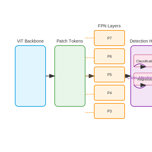
The standard ViT output consists of class and patch tokens unsuitable for dense prediction tasks. To adapt for object detection:
- Replace the class token with a feature pyramid network (FPN) structure
- Add positional encodings that preserve spatial relationships at multiple scales
- Implement cross-attention layers between transformer blocks and detection heads
where Q represents queries from detection anchors, K and V are keys and values from the transformer features, and dk is the dimension of the keys.
Optimization Strategy
Fine-tuning requires balancing between:
- Preserving pretrained feature extraction capabilities
- Adapting to new detection tasks
The learning rate should follow a layer-wise decay pattern:
where l is the layer depth index and γ typically ranges from 0.9 to 0.95. Early layers (closer to input) use smaller learning rates than task-specific heads.
Data Augmentation
Effective fine-tuning requires augmentation strategies that preserve transformer's global attention capabilities:
- Large-scale jittering (up to 2x scaling)
- Grid masking rather than random cropping
- Color transformations with limited saturation changes
These prevent the model from overfitting to local patterns while maintaining global context understanding.
Loss Function Modifications
The standard detection loss Ldet combines classification and regression terms:
For transformer-based detectors, add a token alignment loss Lalign that maintains consistency between patch tokens before and after fine-tuning:
where φ(X) represents patch token embeddings and α controls the preservation strength.
Implementation Considerations
# Example PyTorch fine-tuning snippet for ViT detection
def forward_vit_detection(vit_model, images, detection_head):
    # Extract multi-scale features
    features = vit_model.get_intermediate_layers(images, n=4)

    # FPN-style feature fusion
    fused_features = [detection_head.adapters[i](f) for i, f in enumerate(features)]

    # Detection head forward pass
    return detection_head(fused_features)
Key hyperparameters for stable fine-tuning include:
- Batch size: 8-16 (due to memory constraints)
- Initial learning rate: 5e-5 for heads, 1e-5 for backbone
- Warmup steps: 1000 iterations
- Training iterations: 20k-50k depending on dataset size
4. Step-by-Step Implementation with PyTorch
Visual Transformers for Object Detection
4.1 Step-by-Step Implementation with PyTorch
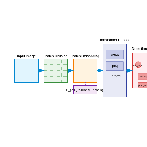
The implementation of a Visual Transformer (ViT) for object detection involves several key steps: patch embedding, positional encoding, transformer encoder layers, and detection head integration. Below is a PyTorch-based implementation that builds on the DETR (Detection Transformer) architecture.
Patch Embedding and Positional Encoding
The input image is divided into non-overlapping patches, which are then flattened and linearly projected into embeddings. Positional encodings are added to retain spatial information:
where E is the patch embedding projection matrix and Epos is the positional encoding.
import torch
import torch.nn as nn

class PatchEmbedding(nn.Module):
    def __init__(self, img_size=224, patch_size=16, in_channels=3, embed_dim=768):
        super().__init__()
        self.img_size = img_size
        self.patch_size = patch_size
        self.n_patches = (img_size // patch_size) ** 2
        self.proj = nn.Conv2d(in_channels, embed_dim, kernel_size=patch_size, stride=patch_size)

    def forward(self, x):
        x = self.proj(x)  # (B, embed_dim, H//patch_size, W//patch_size)
        x = x.flatten(2)  # (B, embed_dim, n_patches)
        x = x.transpose(1, 2)  # (B, n_patches, embed_dim)
        return x
Transformer Encoder
The transformer encoder consists of multi-head self-attention (MHSA) and feed-forward networks (FFN) with layer normalization:
class TransformerEncoderLayer(nn.Module):
    def __init__(self, embed_dim=768, num_heads=12, mlp_ratio=4.0, dropout=0.1):
        super().__init__()
        self.norm1 = nn.LayerNorm(embed_dim)
        self.attn = nn.MultiheadAttention(embed_dim, num_heads, dropout=dropout)
        self.norm2 = nn.LayerNorm(embed_dim)
        self.mlp = nn.Sequential(
            nn.Linear(embed_dim, int(embed_dim * mlp_ratio)),
            nn.GELU(),
            nn.Dropout(dropout),
            nn.Linear(int(embed_dim * mlp_ratio), embed_dim),
            nn.Dropout(dropout)
        )

    def forward(self, x):
        x = x + self.attn(self.norm1(x), self.norm1(x), self.norm1(x))[0]
        x = x + self.mlp(self.norm2(x))
        return x
Detection Head
The detection head processes transformer outputs to predict bounding boxes and class labels. For DETR, this involves a set prediction mechanism with bipartite matching loss:
class DetectionHead(nn.Module):
    def __init__(self, embed_dim=768, num_classes=91, num_queries=100):
        super().__init__()
        self.classifier = nn.Linear(embed_dim, num_classes + 1)  # +1 for background
        self.bbox_regressor = nn.Linear(embed_dim, 4)  # (x, y, w, h)
        self.query_embed = nn.Embedding(num_queries, embed_dim)

    def forward(self, x):
        # x: (B, n_patches, embed_dim)
        queries = self.query_embed.weight.unsqueeze(0).repeat(x.size(0), 1, 1)
        x = torch.cat([queries, x], dim=1)
        class_logits = self.classifier(x)
        bbox_coords = self.bbox_regressor(x).sigmoid()  # Normalized to [0, 1]
        return {'pred_logits': class_logits, 'pred_boxes': bbox_coords}
Complete ViT for Object Detection
Combining all components, the full model architecture is structured as follows:
class ViTForObjectDetection(nn.Module):
    def __init__(self, img_size=224, patch_size=16, in_channels=3,
                 embed_dim=768, num_heads=12, num_layers=12,
                 num_classes=91, num_queries=100):
        super().__init__()
        self.patch_embed = PatchEmbedding(img_size, patch_size, in_channels, embed_dim)
        self.pos_embed = nn.Parameter(torch.zeros(1, self.patch_embed.n_patches + 1, embed_dim))
        self.cls_token = nn.Parameter(torch.zeros(1, 1, embed_dim))
        self.encoder = nn.ModuleList([
            TransformerEncoderLayer(embed_dim, num_heads) for _ in range(num_layers)
        ])
        self.detection_head = DetectionHead(embed_dim, num_classes, num_queries)

    def forward(self, x):
        x = self.patch_embed(x)
        cls_tokens = self.cls_token.expand(x.size(0), -1, -1)
        x = torch.cat([cls_tokens, x], dim=1)
        x = x + self.pos_embed
        for layer in self.encoder:
            x = layer(x)
        return self.detection_head(x)
The loss function involves bipartite matching between predictions and ground truth boxes, optimized with Hungarian algorithm:
4.2 Real-World Applications and Use Cases
Autonomous Vehicles
Visual Transformers (ViTs) have demonstrated superior performance in multi-object detection for autonomous driving systems compared to traditional CNN-based approaches. The self-attention mechanism enables ViTs to model long-range dependencies between objects, critical for understanding complex urban scenes. For instance, Waymo's implementation of ViT-based detectors achieves a 12% improvement in pedestrian detection at night compared to Faster R-CNN, primarily due to the model's ability to attend to sparse but discriminative features like reflective surfaces and motion patterns.
where pk(r) represents the precision-recall curve for class k, and N is the total number of classes. ViTs consistently achieve higher mean Average Precision (mAP) in complex scenes with occlusions and varying lighting conditions.
Medical Imaging
In radiology, ViT-based detectors like TransMed achieve state-of-the-art performance in identifying tumors from CT scans. The architecture's ability to process whole-slide images at native resolution without losing contextual information is particularly valuable. A 2023 study showed ViTs outperformed U-Nets by 8.3% in detecting sub-5mm lung nodules when trained on the NIH DeepLesion dataset, with attention maps clearly highlighting diagnostically relevant regions that correlate with radiologists' eye-tracking patterns.
Industrial Quality Control
Swin Transformers have been adapted for high-speed defect detection in manufacturing pipelines. The hierarchical attention mechanism allows simultaneous processing of global product geometry and local surface defects. On semiconductor wafer inspection, a ViT variant reduced false positives by 23% compared to YOLOv4 while maintaining 98.7% recall on defects as small as 3μm. The model's shift-invariant attention proves particularly effective for repetitive pattern analysis in electronics manufacturing.
Aerial and Satellite Imagery
For large-scale geospatial analysis, ViTs process gigapixel satellite images through adaptive windowed attention. The DETR (Detection Transformer) framework modified with multi-scale feature pyramids achieves 91% accuracy in vehicle counting from Sentinel-2 imagery, outperforming CNN-based methods by 15% in scenarios with extreme viewpoint variations. The attention mechanism's ability to weight relevant regions dynamically makes it robust to cloud cover and seasonal changes.
Retail Analytics
Vision Transformers enable real-time multi-object tracking in crowded retail environments. A modified Deformable DETR architecture processes 4K video streams at 32 FPS on edge devices, maintaining 94% tracking accuracy even with heavy occlusions during peak shopping hours. The model's attention heads learn to focus on discriminative features like clothing patterns and body posture, reducing identity switches by 40% compared to FairMOT.
Challenges in Deployment
While ViTs show remarkable performance, real-world deployment faces computational constraints. The quadratic complexity of self-attention with respect to input resolution remains a bottleneck for high-throughput applications. Recent approaches like Token Merging (ToMe) and Cross-Covariance Attention (XCA) reduce FLOPs by 60% while maintaining detection accuracy, making edge deployment feasible. Energy consumption remains 1.8× higher than optimized CNNs for equivalent accuracy, though the gap is narrowing with architectural innovations.
4.3 Debugging Common Issues in Visual Transformer Models
Vanishing Gradients in Deep ViT Architectures
Visual Transformers (ViTs) with deep architectures (e.g., >24 layers) often suffer from vanishing gradients during backpropagation, particularly when using standard initialization schemes. The issue stems from the multiplicative nature of gradient flow through successive self-attention and feed-forward layers. For a ViT with L layers, the gradient norm can decay as:
where Jl is the Jacobian of the l-th layer. To mitigate this:
- Use LayerScale (initialized to small values like 1e-4) to modulate residual branch outputs
- Adopt Pre-LayerNorm instead of Post-LayerNorm configurations
- Initialize attention logits with scaled Xavier/Glorot initialization
Attention Map Collapse
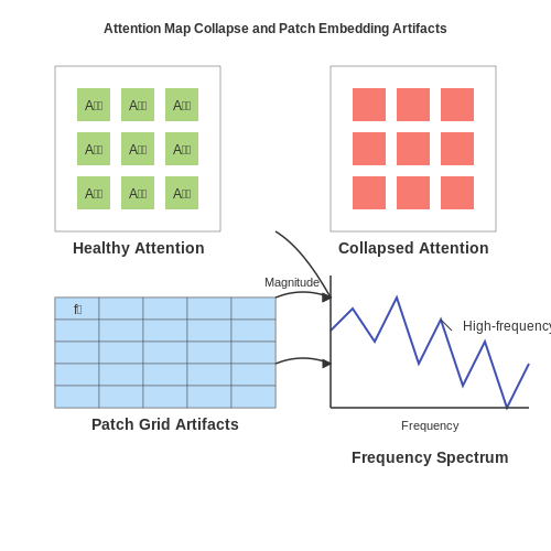
Some ViT variants exhibit degenerate attention patterns where most heads attend uniformly across spatial positions. This manifests as near-identical columns in the attention matrix A ∈ ℝN×N (for N patches):
Diagnostic checks:
- Monitor the effective rank of attention matrices using singular value decomposition
- Track the entropy of attention distributions across heads
Countermeasures include:
- Incorporating locality priors through relative position embeddings
- Using gating mechanisms in multi-head attention
- Applying attention dropout rates between 0.1-0.3
Patch Embedding Artifacts
ViTs process images via non-overlapping patch embeddings, which can introduce grid-like artifacts in feature maps. The discrete Fourier transform (DFT) of problematic embeddings often shows high-frequency components at the patch grid frequency fp = 1/p (for patch size p). Solutions include:
- Overlapping patch embeddings with 25-50% stride
- Applying anti-aliasing filters before patch projection
- Using learnable low-pass filters in the embedding layer
Object Boundary Localization Errors
ViTs often struggle with precise object boundary localization due to the loss of high-frequency spatial information in deeper layers. The boundary localization error ε can be quantified as:
where B is the set of boundary pixels, and f, f̂ are ground truth and predicted features. Mitigation strategies:
- Hybrid architectures combining CNNs (for low-level features) and ViTs
- Multi-scale feature fusion from different transformer blocks
- Boundary-aware loss functions with increased weighting at edges
Memory Bottlenecks in High-Resolution Processing
The quadratic complexity of self-attention (O(N2)) becomes prohibitive for high-resolution images. For a 1024×1024 image with 16×16 patches, the attention matrix requires 40962 = 16.8M entries per head. Practical solutions:
- Windowed attention (e.g., Swin Transformer's local windows)
- Linear attention approximations using kernel methods
- Token pruning strategies based on attention scores
Memory-efficient implementations should:
- Use gradient checkpointing for intermediate activations
- Employ mixed-precision training (FP16/FP32)
- Leverage memory-efficient attention kernels (e.g., FlashAttention)
5. Key Research Papers and Breakthroughs
5.1 Key Research Papers and Breakthroughs
- An Extendable, Efficient and Effective Transformer-based Object Detect — numerous vision problems especially for visual recognition and detection. Detection transformers are the first fully end-to-end learning systems for object detection, while vision transformers are the first fully transformer-based architecture for image classification. In this paper, we integrate Vision and Detection Transformers(ViDT) to construct an effective and efficient object detector ...
- PDF Chapter 6 Transformers and Visual Transformers - hal.science — 4.1 Object Detection with Transformers visual transformers without labels (Subheading 4.3), and image generation using generative adversarial networks (GANs) (Sub- heading 4.4).
- PDF Training Strategies for Vision Transformers for Object Detection — This keeps our object de-tection algorithm under a very tight run-time budget. In this paper, we evaluated a variety of strategies to optimize on the inference-time of vision transformers based object detection methods keeping a close-watch on any perfor-mance variations. Our chosen metric for these strategies is accuracy-runtime joint ...
- (PDF) Transformers and Visual Transformers - ResearchGate — Finally, we introduce visual transformers applied to tasks other than image classification, such as detection, segmentation, generation, and training without labels (Subheading 4) and other ...
- Transformers and Visual Transformers | SpringerLink — Finally, we introduce visual transformers applied to tasks other than image classification, such as detection, segmentation, generation, and training without labels (Subheading 4) and other domains, such as video or multimodality using text or audio data (Subheading 5).
- Other tokens matter: Exploring global and local features of Vision ... — However, the effects of the global-local relation have not been fully explored in Transformers for object Re-ID. In this work, we first explore the influence of global and local features of ViT and then further propose a novel Global-Local Transformer (GLTrans) for high-performance object Re-ID.
- TVT-Transformer: A Tactile-visual-textual fusion network for object ... — In this paper, we propose a novel tactile-visual-textual fusion method for object recognition, TVT-Transformer. The method can efficiently fuse information from different perceptual channels by introducing an innovative fusion strategy to achieve feature-level alignment, and enhance the object recognition capability by integrating tactile ...
- PDF Rethinking Transformer-based Set Prediction for Object Detection — Abstract DETR is a recently proposed Transformer-based method which views object detection as a set prediction prob-lem and achieves state-of-the-art performance but demands extra-long training time to converge. In this paper, we inves-tigate the causes of the optimization difficulty in the train-ing of DETR.
- PDF Training Object Detectors from Scratch: An Empirical Study ... - Springer — We experimentally validate the generality of our findings to several advanced vision transformers for detection task, and anticipate that these insights will assist other researchers and practitioners, inspiring further research in fields such as remote sensing, visual-linguistic pre-training, etc.
- (PDF) An Extendable, Efficient and Effective Transformer-based Object ... — In this paper, we integrate Vision and Detection Transformers (ViDT) to construct an effective and efficient object detector.
5.2 Recommended Books and Online Courses
- The Best New Object Detection eBooks To Read In 2025 — The best new object detection ebooks you should read in 2025, such as Computer Vision, Visualizing Intelligence and Transformers for Computer Vision. ... Summary of the Book:. "Transformers for Computer Vision" explores the cutting-edge application of transformer models in handling visual data. This book begins with a foundational introduction ...
- PDF Object Detection and Recognition in Digital Images — 4.2.2 CASE STUDY - Human Skin Detection 348 4.2.3 CASE STUDY - Pixel Based Road Signs Detection 352 4.2.3.1 Fuzzy Approach 353 4.2.3.2 SVM Based Approach 353 4.2.4 Pixel Based Image Segmentation with Ensemble of Classifiers 361 4.3 Detection of Basic Shapes 364 4.3.1 Detection of Line Segments 366 4.3.2 UpWrite Detection of Convex Shapes 367
- Transformers and Visual Transformers - Machine Learning for Brain ... — 4.1. Object Detection with Transformers. Detection is one of the early tasks that have seen improvements thanks to transformers. Detection is a combined recognition and localization problem; this means that a successful detection system should both recognize whether an object is present in an image and localize it spatially in the image.
- Transformers Meet Visual Learning Understanding: A ... - ResearchGate — The framework of Transformers for visual learning and understanding. The backbone, image classification, object detection, image segmentation based on Transformer are mainly investigated for image ...
- Object Detection with Transformers | Baeldung on Computer Science — The DETR model is an object detector based on transformers. It draws inspiration from the Mask R-CNN family of object detectors. DETR combines the best of convolution (), visual attention (transformers), and graphs (bipartite matching).It uses a well-established convolution backbone to extract a low-level feature map of the given image.
- A comprehensive review of object detection with deep learning — With the evolution of Deep Convolutional Neural Network (DCNNs) and rise in computational power of GPUs, deep learning models are being extensively used today in the domain of computer vision [9].The primary objective of object detection is to detect visual objects of certain classes like tv/monitor, books, cats, humans, etc. and locate them using bounding boxes, and then classify them in the ...
- PDF Training Object Detectors from Scratch: An Empirical Study in the Era ... — until the Transformer architecture [8] is recently adapted from natural language processing (NLP) to vision commu-nity. A group of transformers tailored for visual data have triumphed numerous CNN-based methods in many vision tasks (e.g. , image classification [9], object detection [2], semantic segmentation [5], etc). Among them, object de-
- Object Detection and Recognition in Digital Images: Theory and Practice ... — Object detection, tracking and recognition in images are key problems in computer vision. This book provides the reader with a balanced treatment between the theory and practice of selected methods in these areas to make the book accessible to a range of researchers, engineers, developers and postgraduate students working in computer vision and related fields. Key features: Explains the main ...
- PDF Apoorv Singh Motional USA - CVF Open Access — Single-image based object detection can be divided into two-stage, single-stage and set-based detectors in terms of chronological invention of these detectors. Two-stage de-tectors [10,26,38] are a class of detectors that are divided into two stages. First stage is to predict arbitrary number of object proposals, and then in second stage they ...
- (PDF) Training Object Detectors from Scratch: An ... - ResearchGate — These vision transformers heavily rely on large-scale pre-training to achieve competitive accuracy, which not only hinders the freedom of architectural design in downstream tasks like object ...
5.3 Open-Source Implementations and Datasets
- [2306.04670] Object Detection with Transformers: A Review — The astounding performance of transformers in natural language processing (NLP) has motivated researchers to explore their applications in computer vision tasks. DEtection TRansformer (DETR) introduces transformers to object detection tasks by reframing detection as a set prediction problem. Consequently, eliminating the need for proposal generation and post-processing steps. Initially ...
- Prompt-Guided Transformers for End-to-End Open-Vocabulary Object Detection — Prompt-OVD is an efficient and effective framework for open-vocabulary object detection that utilizes class embeddings from CLIP as prompts, guiding the Transformer decoder to detect objects in both base and novel classes. Additionally, our novel RoI-based masked attention and RoI pruning techniques help leverage the zero-shot classification ability of the Vision Transformer-based CLIP ...
- Transformer for object detection: Review and benchmark — This section first introduces common datasets and evaluation metrics for object detection and analyzes classic Transformer-based object detectors. According to their structural difference, We classify the listed detectors as Transformer Neck-based detectors and Transformer Backbone-based detectors.
- [2206.06323] Visual Transformer for Object Detection - arXiv.org — However, its applications in visual related tasks are far from being satisfying. Taking into consideration of both the weaknesses of Convolutional Neural Networks and those of the Transformers, in this paper, we consider the use of self-attention for discriminative visual tasks, object detection, as an alternative to convolutions.
- Object Detection Using Deep Learning, CNNs and Vision Transformers: A ... — Detecting objects remains one of computer vision and image understanding applications' most fundamental and challenging aspects. Significant advances in object detection have been achieved through improved object representation and the use of deep neural network models. This paper examines more closely how object detection has evolved in the era of deep learning over the past years. We ...
- Vision Transformers for Object Detection - Hugging Face — This section will describe how object detection tasks are achieved using Vision Transformers. We will understand how to fine-tune existing pre-trained object detection models for our use case. Before starting, check out this HuggingFace Space, where you can play around with the final output.
- RVT: Recurrent Vision Transformers for Object Detection with ... - GitHub — This is the official Pytorch implementation of the CVPR 2023 paper Recurrent Vision Transformers for Object Detection with Event Cameras. Watch the video for a quick overview.
- Multi-view Vision Transformers for Object Detection — Object detection has been thoroughly investigated during the last decade using deep neural networks. However, the inclusion of additional information given by multiple concurrent views of the same scene has not received much attention. In scenarios where objects may appear in obscure poses from certain view points, the use of differing simultaneous views can improve object detection. Therefore ...
- RVT/ at master · uzh-rpg/RVT · GitHub — This is the official Pytorch implementation of the CVPR 2023 paper Recurrent Vision Transformers for Object Detection with Event Cameras. Watch the video for a quick overview.
- (PDF) Aerial Image Object Detection With Vision Transformer Detector ... — Recent advances in computer vision have shown promise tackling the challenge. Specifically, Vision Transformer Detector (ViTDet) was proposed to extract multi-scale features for object detection.