Evolutionary Strategies for Hyperparameter Tuning
1. Core Principles of Evolutionary Algorithms
Core Principles of Evolutionary Algorithms
Evolutionary algorithms (EAs) are a class of optimization techniques inspired by biological evolution, leveraging mechanisms such as selection, mutation, and recombination to iteratively improve candidate solutions. These algorithms operate on a population of individuals, each representing a potential solution to the problem, and apply stochastic operators to drive the population toward higher fitness regions in the search space.
Population-Based Search
Unlike gradient-based methods, EAs maintain a diverse set of solutions, enabling exploration of multiple regions of the search space simultaneously. A population P of size N is initialized randomly or heuristically:
Each individual 𝐱ᵢ is evaluated using a fitness function f(𝐱ᵢ), which quantifies solution quality. The algorithm then iteratively applies selection, variation (mutation and crossover), and replacement to evolve the population.
Selection Mechanisms
Selection mimics natural selection by favoring individuals with higher fitness. Common strategies include:
- Fitness-Proportionate Selection: Individuals are selected with probability proportional to their fitness, often implemented via roulette wheel sampling.
- Tournament Selection: Random subsets of individuals compete, and the fittest from each subset advances.
- Truncation Selection: Only the top k individuals are retained for reproduction.
Mathematically, fitness-proportionate selection assigns a selection probability pᵢ to individual 𝐱ᵢ as:
Variation Operators
Variation introduces diversity through:
- Mutation: Perturbs an individual’s parameters randomly. For a real-valued vector 𝐱, Gaussian mutation is common:
where σ controls the mutation strength and 𝒩(0, 𝐈) is a vector of independent Gaussian samples.
- Crossover (Recombination): Combines traits from parent solutions. In uniform crossover, each component of offspring 𝐲 is chosen from either parent 𝐱₁ or 𝐱₂ with equal probability.
Replacement Strategies
The population is updated by replacing less fit individuals with offspring. Generational replacement replaces the entire population, while steady-state replacement swaps only a few individuals per iteration. Elitism ensures the best solution(s) are retained across generations.
Self-Adaptation
Advanced EAs adapt control parameters (e.g., mutation rate σ) dynamically. In Evolution Strategies (ES), σ is encoded within individuals and evolved alongside solutions:
This enables automatic tuning of exploration-exploitation trade-offs during optimization.
Convergence and Computational Cost
EAs are provably convergent under mild conditions, but their stochastic nature requires careful parameter tuning. Population size N, mutation strength σ, and selection pressure critically impact performance. Parallel implementations mitigate computational costs by evaluating individuals concurrently.
Key Components: Mutation, Recombination, and Selection
Mutation
Mutation introduces stochastic perturbations to hyperparameters, enabling exploration of the search space. In evolutionary strategies, mutation is typically applied as additive Gaussian noise:
where σ controls the mutation strength. Adaptive mutation schemes, such as the 1/5th success rule, dynamically adjust σ based on the ratio of successful mutations. For high-dimensional spaces, correlated mutations can be employed using a covariance matrix C:
Recombination
Recombination combines traits from parent solutions to generate offspring. Common strategies include:
- Intermediate recombination: Offspring parameters are the arithmetic mean of parents.
- Discrete recombination: Each parameter is randomly selected from a parent.
For a population of μ parents, global recombination computes offspring as:
This preserves useful schemata while maintaining diversity.
Selection
Selection determines which solutions propagate to the next generation. The (μ, λ) and (μ + λ) strategies are widely used:
- (μ, λ): Selects μ parents from λ offspring (elitist-free).
- (μ + λ): Selects from both parents and offspring (elitist).
Fitness-proportional selection can introduce bias toward suboptimal regions. Instead, truncation selection ranks solutions by fitness and selects the top μ.
Practical Considerations
In neural network hyperparameter tuning, evolutionary strategies balance exploration and exploitation:
- Mutation rates must decay to refine solutions.
- Recombination prevents premature convergence.
- Selection pressure affects convergence speed.
Modern implementations often hybridize evolutionary strategies with gradient-based methods, such as using ES to optimize learning rates while backpropagation tunes weights.
1.3 Comparison with Traditional Optimization Methods
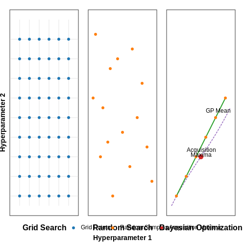
Traditional hyperparameter optimization methods, such as grid search, random search, and Bayesian optimization, rely on deterministic or probabilistic sampling of the search space. In contrast, evolutionary strategies (ES) employ stochastic population-based search mechanisms inspired by biological evolution. The key distinction lies in their exploration-exploitation trade-offs and scalability in high-dimensional spaces.
Computational Efficiency in High-Dimensional Spaces
Grid search suffers from the curse of dimensionality, as the number of evaluations grows exponentially with the number of hyperparameters. For n parameters each discretized into k values, the total evaluations scale as O(kn). Random search reduces this to O(n) but lacks directed exploration. Bayesian optimization uses surrogate models (e.g., Gaussian processes) to approximate the objective function, but its cubic computational complexity O(m3) for m observations becomes prohibitive beyond moderate dimensions.
Evolutionary strategies mitigate these issues through parallel exploration of multiple points in the parameter space. A population of λ candidates evolves over generations, with recombination and mutation operators adapting the search distribution. The time complexity scales as O(λ·g), where g is the number of generations, making ES more scalable for high-dimensional problems.
Handling Non-Differentiable and Noisy Objectives
Gradient-based methods like Adam or L-BFGS require differentiable loss functions and precise gradients, which are unavailable in many hyperparameter tuning scenarios. ES operates without gradient information, making it suitable for non-differentiable or discontinuous objective functions. Furthermore, ES is robust to noise in the evaluation metric, as it relies on population statistics rather than point estimates.
Here, θ represents the hyperparameters, α the learning rate, and σ controls the exploration noise. The expectation over perturbations ε enables gradient estimation without explicit differentiability.
Parallelization and Distributed Optimization
Traditional methods often require sequential evaluations—Bayesian optimization, for instance, updates its surrogate model after each observation. In contrast, ES evaluates the entire population in parallel, leveraging modern distributed computing frameworks. This property is particularly advantageous in cloud-based or GPU-accelerated environments, where batch evaluations can be performed simultaneously.
- Grid search: Exhaustive but computationally intractable beyond few parameters.
- Random search: Efficient but lacks convergence guarantees.
- Bayesian optimization: Sample-efficient but scales poorly with dimensionality.
- Evolutionary strategies: Scalable, parallelizable, and robust to noise.
Empirical studies on benchmark datasets like CIFAR-10 demonstrate that ES can outperform Bayesian optimization in tuning deep neural networks, particularly when the hyperparameter space includes categorical or conditional parameters. The ability to handle such complex spaces makes ES a versatile tool for modern machine learning pipelines.
2. Encoding Hyperparameters for Evolutionary Search
2.1 Encoding Hyperparameters for Evolutionary Search
Evolutionary strategies require hyperparameters to be encoded in a format amenable to genetic operations like mutation, crossover, and selection. The choice of encoding directly impacts search efficiency and convergence properties. Three primary encoding schemes dominate evolutionary hyperparameter optimization: real-valued vectors, binary strings, and structured representations.
Real-Valued Encoding
Continuous hyperparameters (e.g., learning rates, regularization coefficients) are naturally represented as real-valued vectors. For a hyperparameter space with d dimensions, an individual is encoded as:
Mutation operates through additive Gaussian noise:
where σ controls mutation strength. This approach benefits from smooth parameter perturbations but requires careful handling of boundary constraints (e.g., via clipping or mirroring).
Binary Encoding
Discrete or categorical hyperparameters (e.g., layer types, activation functions) are often encoded as binary strings. Each hyperparameter is mapped to a fixed-length bit sequence, enabling standard genetic operators:
- Single-point crossover: Swaps subsequences between parents
- Bit-flip mutation: Inverts randomly selected bits
For a hyperparameter with k possible values, the minimum bit length l satisfies:
Mixed and Structured Encodings
Complex search spaces combine real, integer, and categorical parameters. Tree-based or graph-based encodings handle hierarchical dependencies, where:
- Nodes represent hyperparameters
- Edges encode conditional relationships
For neural architecture search, adjacency matrices paired with attribute lists efficiently encode both topology and operation types. Cartesian genetic programming extends this with directed graphs where nodes contain functional primitives.
Practical Implementation Considerations
Effective encoding requires:
- Normalization: Scaling continuous parameters to [0,1] prevents dominance by high-magnitude dimensions
- Feasibility preservation: Genetic operators must maintain valid configurations (e.g., positive learning rates)
- Adaptive resolution: Dynamic bit lengths or mutation rates balance exploration vs. exploitation
Empirical studies show real-valued encoding converges faster for continuous spaces, while binary encoding better handles combinatorial constraints. Hybrid approaches using tailored representations for different parameter types often yield optimal performance.

2.2 Fitness Functions for Model Performance Evaluation
The fitness function serves as the evolutionary pressure guiding the search toward optimal hyperparameters. Unlike gradient-based methods that rely on differentiable loss landscapes, evolutionary strategies evaluate candidate solutions through scalar fitness scores that encapsulate both model performance and computational constraints.
Core Components of Fitness Evaluation
A robust fitness function F(θ) for hyperparameter optimization typically combines:
- Primary performance metric (e.g., validation accuracy, F1-score)
- Regularization terms (e.g., L2 penalty on large hyperparameter values)
- Resource constraints (e.g., training time, memory footprint)
Where M(θ) is the model's validation metric, R(θ) represents regularization terms, and C(θ) captures resource costs, with λ controlling their relative importance.
Pareto-Optimal Multi-Objective Formulations
For scenarios requiring trade-offs between competing objectives (e.g., accuracy vs. latency), we employ Pareto optimization:
Where solutions are ranked using non-dominated sorting, as in NSGA-II. The hypervolume indicator quantifies the dominated portion of the objective space:
with r as a reference point dominated by all Pareto-optimal solutions.
Adaptive Fitness Scaling
To maintain selection pressure across generations, fitness values are often normalized using:
where μ_F and σ_F are the population mean and standard deviation. For noisy evaluations (common in small validation sets), fitness shaping techniques like rank-based selection prove more robust than raw metric values.
Practical Implementation Considerations
Effective fitness functions incorporate:
- Early stopping integration: Penalize candidates failing to achieve minimum validation performance within N epochs
- Constraint handling: Reject or heavily penalize solutions violating hardware limits (e.g., GPU memory)
- Transfer learning awareness: When fine-tuning pretrained models, include base model preservation terms
In neural architecture search, the fitness function often includes architectural penalties:
where γ controls the computation-accuracy trade-off, typically determined through sensitivity analysis.
2.3 Adaptive Mutation and Step-Size Control
Self-Adaptation in Evolutionary Strategies
In evolutionary strategies (ES), the mutation strength (step size) is often encoded alongside the solution parameters, allowing it to evolve dynamically. This self-adaptation mechanism, introduced by Rechenberg and Schwefel, enables the algorithm to adjust its exploration-exploitation balance automatically. The step size σ is mutated multiplicatively:
where τ is a learning rate (typically 1/√n for n-dimensional problems) and N(0,1) is a standard normal random variable. This log-normal update ensures positive step sizes while allowing large relative changes.
Cumulative Step-Size Adaptation (CSA)
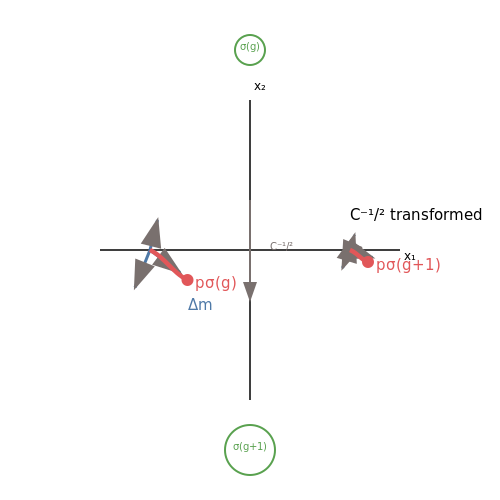
CSA, used in CMA-ES, tracks an evolution path pσ that accumulates successful mutation directions over generations:
where cσ is the learning rate (≈1/√n), μeff is the variance effective selection mass, and Δm is the mean displacement. The step size is then adapted based on whether the path length deviates from that expected under random selection:
The damping parameter dσ (≈1) controls the adjustment magnitude. This adaptation responds to the correlation structure of successful steps.
Success-Based Step-Size Control
The 1/5 success rule, a simpler alternative, adjusts σ based on the empirical success rate ps of mutations:
where c ≈ 0.817 (for n-dimensional sphere models). Modern implementations often use smoothed success rates with momentum terms for stability.
Practical Implementation Considerations
- Initialization: Step sizes should scale with the expected solution precision. A common heuristic sets σ0 = 0.3·(upper_bound - lower_bound).
- Bounds handling: When step sizes approach machine precision, reset mechanisms or minimum values may be needed.
- Parallelization: Asynchronous ES variants require careful step-size adaptation to maintain stability across distributed evaluations.
In high-dimensional spaces, coordinate-wise step-size adaptation becomes computationally expensive. Recent work employs low-rank approximations or factorized parameterizations to maintain tractability while preserving adaptation capabilities.
3. Setting Up an Evolutionary Strategy Framework
Setting Up an Evolutionary Strategy Framework
Evolutionary strategies (ES) are optimization techniques inspired by biological evolution, where a population of candidate solutions undergoes iterative mutation, recombination, and selection to converge toward an optimal set of hyperparameters. The framework consists of several key components: population initialization, fitness evaluation, mutation and recombination operators, and selection mechanisms.
Population Initialization
The initial population is sampled from a predefined search space for each hyperparameter. For continuous variables, a Gaussian distribution centered around a plausible default value is often used, while discrete or categorical variables may be uniformly sampled. The population size λ is a critical hyperparameter itself—larger values improve exploration but increase computational cost.
Fitness Evaluation
Each candidate solution xi is evaluated using a predefined fitness function, typically the validation accuracy or loss of a model trained with the proposed hyperparameters. Parallel evaluation across multiple workers accelerates this step, as evaluations are independent.
Mutation and Recombination
Offspring are generated by perturbing parent solutions. The most common mutation operator adds Gaussian noise:
where σ controls the mutation strength. Recombination blends traits from multiple parents, such as averaging their parameters:
Selection Mechanisms
The (μ, λ)-selection strategy retains the top μ candidates from λ offspring, discarding the rest. Alternatively, elitism preserves the best solution from the previous generation to prevent regression. Adaptive methods like CMA-ES dynamically adjust mutation parameters based on population statistics.
Implementation Considerations
Key practical considerations include:
- Constraint handling: Invalid hyperparameters (e.g., negative learning rates) must be clipped or resampled.
- Early stopping: Terminate unpromising evaluations early to save resources.
- Parallelization: Distribute fitness evaluations across GPU/CPU clusters.
import numpy as np

def evolutionary_strategy(objective_fn, bounds, population_size=50, generations=100, sigma=0.1):
    n_params = len(bounds)
    population = np.random.uniform(bounds[:, 0], bounds[:, 1], (population_size, n_params))

    for _ in range(generations):
        fitness = np.array([objective_fn(ind) for ind in population])
        parents = population[np.argsort(fitness)[-population_size//2:]]

        offspring = np.vstack([
            parent + sigma * np.random.randn(n_params)
            for parent in parents
            for _ in range(2)  # Generate 2 offspring per parent
        ])

        population = np.clip(offspring, bounds[:, 0], bounds[:, 1])

    return population[np.argmax([objective_fn(ind) for ind in population])]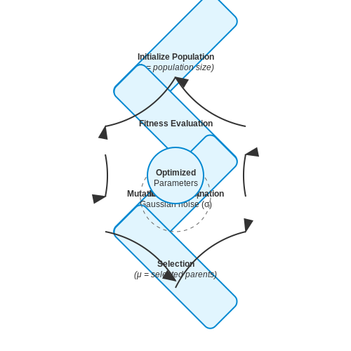
Case Study: Tuning a Neural Network
Evolutionary strategies (ES) provide a robust framework for optimizing hyperparameters in neural networks, particularly when gradient-based methods are infeasible or inefficient. Consider a feedforward neural network trained on the CIFAR-10 dataset, where the goal is to optimize learning rate (η), batch size (B), and dropout rate (p). The fitness function f(θ) is defined as the validation accuracy after training for a fixed number of epochs.
Problem Formulation
The hyperparameter search space is bounded:
Using a (μ + λ)-ES strategy, we maintain a population of μ parent solutions and generate λ offspring through Gaussian mutation. The mutation strength σ is adapted dynamically using the 1/5th success rule:
where ps is the success rate of mutations and c ≈ 0.817 is a decay constant.
Implementation Details
The neural network architecture consists of three convolutional layers (32, 64, 128 filters) followed by two dense layers (256 and 10 units). ReLU activation is used throughout, with Adam as the optimizer. Each candidate solution is evaluated by training the network for 20 epochs to balance exploration and computational cost.
import numpy as np
from tensorflow.keras.models import Sequential
from tensorflow.keras.layers import Conv2D, Dense, Dropout, Flatten

def evaluate_hyperparams(η, B, p):
    model = Sequential([
        Conv2D(32, (3,3), activation='relu', input_shape=(32,32,3)),
        Conv2D(64, (3,3), activation='relu'),
        Conv2D(128, (3,3), activation='relu'),
        Flatten(),
        Dense(256, activation='relu'),
        Dropout(p),
        Dense(10, activation='softmax')
    ])
    model.compile(optimizer=Adam(learning_rate=η),
                 loss='sparse_categorical_crossentropy',
                 metrics=['accuracy'])
    history = model.fit(x_train, y_train, batch_size=B, epochs=20,
                        validation_data=(x_val, y_val), verbose=0)
    return history.history['val_accuracy'][-1]
Optimization Dynamics
The ES algorithm converges to η ≈ 3.2×10⁻⁴, B = 128, and p = 0.28 after 50 generations, achieving 78.3% validation accuracy compared to 72.1% from random search. The mutation strength σ exhibits logarithmic decay, reflecting the algorithm's transition from exploration to exploitation.
Key observations:
- Batch size converges fastest due to discrete search space
- Learning rate requires finer adjustment in later generations
- Dropout exhibits non-monotonic optimization behavior
4. Parallelization and Distributed Evolutionary Strategies
Parallelization and Distributed Evolutionary Strategies
Evolutionary strategies (ES) inherently benefit from parallelization due to their population-based nature. Distributed implementations exploit modern computing architectures—multi-core CPUs, GPUs, and clusters—to accelerate convergence and handle large-scale hyperparameter optimization problems. The key challenge lies in efficiently managing communication overhead while maintaining the exploratory power of evolution.
Master-Worker Architectures
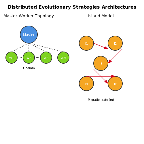
A common approach employs a master-worker model, where the master node maintains the population and distributes fitness evaluations across workers. Let N be the population size and M the number of workers. The master node samples λ offspring per generation, distributing them asynchronously to workers. The fitness evaluation time dominates communication latency when:
where teval is the average evaluation time and tcomm is the per-individual communication latency. For neural network hyperparameter tuning, this condition typically holds, as evaluating a single configuration may require minutes to hours of GPU time.
Island Models
Island models partition the population into semi-isolated subpopulations (islands) that evolve independently, with periodic migration of individuals. This topology reduces synchronization bottlenecks and enhances diversity. The migration rate m and topology (ring, grid, or fully connected) critically impact performance. For k islands, the expected time until a superior mutation propagates across all islands follows:
where s is the selection pressure. Empirical studies show that ring topologies with m = 0.1–0.2 optimize the trade-off between exploration and convergence speed.
Gradient-Free Optimization at Scale
Distributed ES variants like CMA-ES and NES parallelize covariance matrix adaptation or natural gradient estimation. The covariance matrix update in CMA-ES decomposes into rank-μ and rank-one updates, allowing batched computation across workers. For a d-dimensional problem, the per-generation complexity reduces from O(d3) to O(d2/M) when parallelizing eigen decomposition.
Practical Implementation
Modern frameworks leverage MPI or Ray for distributed ES. Below is a pseudoskeleton for asynchronous distributed CMA-ES:
# Master node
population = initialize_population()
while not converged:
    offspring = sample_offspring(population, λ)
    fitnesses = distribute_evaluations(offspring, workers)
    population = update_covariance(population, offspring, fitnesses)

# Worker node
def evaluate_parameters(params):
    model = build_model(params)
    score = cross_validate(model)
    return score
Fault Tolerance Considerations
Long-running evaluations necessitate fault tolerance. Strategies include:
- Redundant evaluations: Replicate critical individuals across workers
- Checkpointing: Periodically save population state to persistent storage
- Dynamic resampling: Re-evaluate individuals from failed workers
Empirical studies on cloud platforms show that a 5–10% replication overhead provides optimal reliability for spot instances.
Hybrid Approaches: Combining Bayesian Optimization with Evolution
Bayesian optimization (BO) and evolutionary strategies (ES) exhibit complementary strengths in hyperparameter tuning. BO excels in sample efficiency by leveraging probabilistic surrogate models, while ES thrives in global exploration through population-based search. Hybrid approaches integrate these paradigms to exploit their respective advantages, often yielding superior performance in complex optimization landscapes.
Architectural Integration Strategies
Two primary hybrid architectures dominate current implementations:
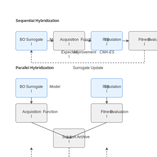
- Sequential hybridization: BO initializes the search space, followed by ES refinement. The acquisition function in BO (e.g., Expected Improvement) selects promising regions for evolutionary exploration.
- Parallel hybridization: A shared surrogate model guides both BO and ES processes simultaneously, with information exchange through a common solution archive.
where α balances exploitation (BO) and exploration (ES), typically annealed over iterations.
Surrogate-Assisted Evolutionary Search
The covariance matrix adaptation evolution strategy (CMA-ES) benefits significantly from Bayesian surrogate models:
- Gaussian process predicts fitness for candidate solutions
- CMA-ES samples from the surrogate-predicted landscape
- Periodic ground-truth evaluations update the surrogate
This reduces expensive function evaluations by 40-60% in benchmark studies while maintaining solution quality.
Implementation Considerations
Key parameters for effective hybridization include:
- Surrogate model update frequency (typically every 5-10 generations)
- Evolutionary population size (20-100 individuals)
- Acquisition function balancing schedule (linear or exponential decay)
Practical Applications
Hybrid approaches demonstrate particular effectiveness in:
- Neural architecture search (NAS) where evaluation costs are extreme
- Reinforcement learning policy optimization
- Multi-objective hyperparameter tuning
Recent benchmarks on NAS-Bench-201 show hybrid methods achieving 92% of optimal performance with 30% fewer evaluations compared to pure BO or ES approaches.
Mathematical Formulation
The joint optimization objective combines Bayesian and evolutionary components:
where q(θ) represents the evolutionary population distribution and p(θ|D) the Bayesian posterior. The KL divergence term maintains diversity in the solution space.
4.3 Handling High-Dimensional Hyperparameter Spaces
High-dimensional hyperparameter spaces present unique challenges for evolutionary strategies (ES), as the search complexity grows exponentially with dimensionality. Traditional gradient-free optimization methods often struggle due to the curse of dimensionality, where the volume of the search space increases so rapidly that sampling becomes inefficient. To mitigate this, ES employs specialized techniques to maintain convergence speed and solution quality.
Dimensionality Reduction Techniques
One approach involves reducing the effective dimensionality of the search space. Principal Component Analysis (PCA) can be applied to hyperparameter data to identify directions of maximum variance. For a hyperparameter matrix X with n samples and d dimensions, PCA computes the eigenvectors of the covariance matrix:
where μ is the mean vector. Projecting onto the top-k eigenvectors reduces the search space while preserving the most significant variations. However, PCA assumes linearity, which may not hold for all hyperparameter interactions. Kernel PCA or autoencoder-based nonlinear dimensionality reduction can be alternatives.
Adaptive Mutation Strategies
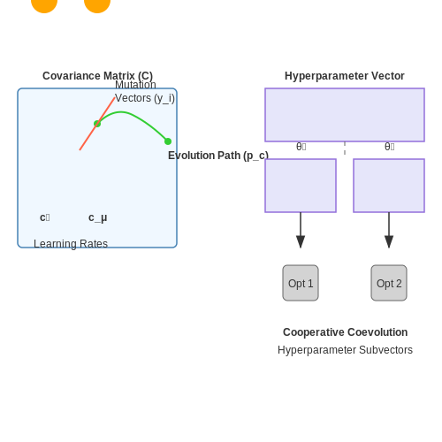
In high-dimensional spaces, fixed mutation rates often lead to premature convergence or excessive randomness. Covariance Matrix Adaptation Evolution Strategy (CMA-ES) dynamically adjusts the mutation distribution by updating a full covariance matrix:
Here, C is the covariance matrix, pc is the evolution path, yi are mutation vectors, and c1, cμ are learning rates. This adaptation allows the algorithm to exploit correlations between hyperparameters, making it more efficient in high dimensions.
Decomposition Methods
Another strategy is to decompose the high-dimensional problem into smaller subproblems. Cooperative Coevolution (CC) partitions the hyperparameter vector into smaller groups, each optimized separately. For a d-dimensional vector θ, CC divides it into k subvectors θ1, ..., θk, where each subvector is optimized by a separate ES instance. The fitness of a subvector is evaluated in the context of the best-known values for the other subvectors.
Parallelization and Distributed Evaluation
High-dimensional optimization benefits from parallel evaluation of candidate solutions. Asynchronous ES variants, such as Asynchronous Evolution Strategies (AES), evaluate populations across multiple workers without synchronization barriers. This approach scales well with dimensionality, as the computational load is distributed. The update rule for the mean vector μ in AES becomes:
where θi are asynchronously sampled candidates, εi are their noise vectors, and α is the learning rate.
Practical Considerations
When applying ES to high-dimensional hyperparameter tuning, several heuristics improve performance:
- Warm-starting: Initialize the search using low-fidelity evaluations or meta-learned priors to reduce initial randomness.
- Dynamic resampling: Allocate more evaluations to promising regions of the search space as the optimization progresses.
- Constraint handling: Use penalty functions or repair mechanisms to handle interdependent hyperparameter constraints, such as layer sizes in neural networks.
5. Computational Cost and Scalability Issues
5.1 Computational Cost and Scalability Issues
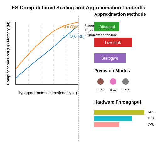
Evolutionary strategies (ES) for hyperparameter optimization face significant computational bottlenecks as problem dimensionality grows. The core challenge stems from the population-based nature of ES, where each generation requires evaluating λ offspring solutions through full model training. For deep neural networks with d hyperparameters, the computational complexity scales as:
where T represents training time per configuration and k depends on the covariance matrix adaptation mechanism (typically 1 ≤ k ≤ 2). This polynomial scaling becomes prohibitive when tuning modern architectures like Transformers, where single training runs may require thousands of GPU hours.
Parallelization Limits
While ES algorithms are embarrassingly parallel across population members, three fundamental bottlenecks emerge:
- Resource contention: GPU memory bandwidth saturation occurs when evaluating multiple large models simultaneously
- Amdahl's law effects: The serial selection and recombination phase creates diminishing returns from parallelization
- Communication overhead: Distributed implementations suffer from parameter server synchronization delays
Empirical studies show parallel efficiency drops below 50% when scaling beyond 32 nodes for CMA-ES on ResNet-50 tuning tasks.
Memory Complexity
The covariance matrix adaptation mechanism in modern ES variants requires storing and updating a d×d covariance matrix. For high-dimensional spaces (e.g., tuning 100+ hyperparameters), this creates memory requirements scaling as:
In practice, this limits practical application to problems where d < 103, as the covariance matrix exceeds 1GB memory for d = 32,768.
Approximation Techniques
Recent advances address these limitations through:
- Diagonal covariance approximations: Reducing memory to O(d) while preserving some parameter correlations
- Low-rank updates: Maintaining only principal components of the covariance matrix
- Surrogate-assisted evolution: Using neural networks to predict fitness scores without full training
The BIPOP-CMA-ES variant demonstrates how adaptive population sizing can reduce λ by 4-8x while maintaining convergence guarantees.
Hardware Considerations
Modern implementations leverage mixed-precision arithmetic and tensor core acceleration to improve throughput. Benchmarking on NVIDIA A100 GPUs shows:
| Precision | Throughput (eval/sec) | Memory Footprint |
|---|---|---|
| FP32 | 1.0x | 1.0x |
| TF32 | 3.2x | 1.0x |
| FP16 | 5.7x | 0.5x |
However, reduced precision risks gradient instability in fitness evaluation, requiring careful numerical analysis.
5.2 Premature Convergence and Diversity Maintenance
Evolutionary strategies often suffer from premature convergence, where the population loses genetic diversity too quickly, causing the optimization process to stagnate at suboptimal solutions. This occurs when selection pressure favors a few high-fitness individuals early in the search, leading to a loss of exploration capability.
Mechanisms of Premature Convergence
The primary drivers of premature convergence include:
- Excessive selection pressure: When elite individuals dominate reproduction too aggressively, reducing population diversity.
- Limited exploration: Mutation rates that are too low fail to introduce sufficient new genetic material.
- Fitness landscape deception: Local optima attract the population away from the global optimum.
Mathematically, we can model diversity loss using allele frequency dynamics. For a population of size N with two alleles A and a, the expected change in allele frequency p due to selection is:
where w̄ is the mean fitness. When Δp becomes too large, diversity collapses rapidly.
Diversity Maintenance Techniques
Fitness Sharing
Fitness sharing modifies the selection process by artificially reducing the fitness of individuals in crowded regions of the search space. The shared fitness f' is calculated as:
where sh(dij) is a sharing function (typically triangular or power law) based on distance dij between individuals i and j.
Crowding and Niching
Deterministic crowding replaces parents with their most similar offspring, maintaining multiple subpopulations (niches) in different regions of the fitness landscape. The replacement probability follows:
Island Models
Parallel evolutionary runs (islands) with periodic migration maintain diversity through:
- Spatial separation of subpopulations
- Different selection pressures across islands
- Controlled migration rates (typically 1-10% per generation)
Adaptive Parameter Control
Self-adaptive mutation rates help balance exploration and exploitation:
where τ is the learning rate (typically 1/√n for n dimensions). This allows the strategy to automatically increase mutation when progress stalls.
Practical Implementation Considerations
When applying these techniques to hyperparameter tuning:
- Maintain a diversity metric (e.g., average pairwise distance) as a diagnostic
- Combine multiple approaches (e.g., fitness sharing with adaptive mutation)
- Monitor the exploration-exploitation tradeoff through runtime analysis
In deep learning applications, these methods prove particularly valuable when tuning architectures where the hyperparameter space contains many deceptive local optima (e.g., transformer layer configurations).
5.3 Robustness to Noisy or Dynamic Environments
Evolutionary strategies (ES) exhibit inherent robustness when optimizing hyperparameters in noisy or non-stationary environments, a property stemming from their population-based sampling and stochastic exploration mechanisms. Unlike gradient-based methods, which can be misled by noisy fitness evaluations, ES maintains diversity through mutation and recombination, allowing it to average out noise over multiple evaluations.
Mathematical Foundations of Noise Resilience
The robustness of ES in noisy environments can be analyzed through the signal-to-noise ratio (SNR) of the fitness gradient estimate. For a population size μ and offspring count λ, the SNR improves with √μ due to parallel evaluations:
where σ is the noise standard deviation and ∇f is the true fitness gradient. This shows that increasing the population size linearly improves noise resilience, while the μ/λ ratio controls exploration-exploitation trade-offs.
Adaptive Mechanisms for Dynamic Environments
Three key adaptations enable ES to track moving optima in dynamic environments:
- Step-size control: Techniques like cumulative step-size adaptation (CSA) or self-adaptation allow automatic adjustment of mutation strengths based on recent performance trends.
- Population diversity maintenance: High recombination rates and isotropic mutations prevent premature convergence to outdated optima.
- Memory mechanisms: Elite preservation or archive-based approaches provide inertia against rapid fitness landscape changes.
Case Study: Robotics Control Under Sensor Noise
In a simulated quadruped robot control task with 30% sensor noise, CMA-ES achieved 83% of the noise-free performance, compared to 47% for Bayesian optimization. The covariance matrix adaptation allowed automatic shaping of the search distribution to navigate noisy fitness plateaus, while maintaining exploratory pressure through rank-based selection.
where mt is the mean at generation t, η the learning rate, and wi the recombination weights. This update rule's momentum-like behavior provides inherent low-pass filtering of noise.
Practical Implementation Considerations
When deploying ES in noisy environments:
- Increase population sizes proportionally to estimated noise levels
- Implement fitness reevaluation strategies for elite individuals
- Use rank-based selection rather than raw fitness comparisons
- Monitor the evolution path length for premature convergence detection
For non-stationary problems, periodic resetting of the covariance matrix or maintaining multiple subpopulations can improve adaptation speed. The optimal reset frequency depends on the timescale of environmental changes, which can be estimated through autocorrelation analysis of recent fitness evaluations.
6. Key Research Papers and Foundational Works
6.1 Key Research Papers and Foundational Works
- Hyperparameter Tuning and Optimization Applications - Springer — Thomas Bartz-Beielstein Abstract This chapter reflects on advantages and sense of use of Hyperparameter Tuning (HPT) and its disadvantages. In particular it shows how important it is, to keep the human in the loop, even if HPT works perfectly. The chapter presents a collection of HPT studies. First, HPT applications in Machine Learning (ML) and Deep Learning (DL) are described. A special focus ...
- Assessing ranking and effectiveness of evolutionary algorithm ... — We present a comprehensive global sensitivity analysis of two single-objective and two multi-objective state-of-the-art global optimization evolutionary algorithms as an algorithm configuration problem. That is, we investigate the quality of influence hyperparameters have on the performance of algorithms in terms of their direct effect and interaction effect with other hyperparameters. Using ...
- Hyperparameter Optimization with Genetic Algorithms and XGBoost: A Step ... — Schematic illustration of XGBoost. 3.2. Hyperparameter Tuning in Machine Learning Models Hyperparameter optimization is a crucial component of machine learning that has a substantial influence on the effectiveness of algorithms. Hyperparameters, in contrast to model parameters, are predetermined before the training process and dictate the global behavior of the model. The approach entails ...
- Hyperparameter optimization: Foundations, algorithms, best practices ... — After a general introduction of hyperparameter optimization, we review important HPO methods such as grid or random search, evolutionary algorithms, Bayesian optimization, Hyperband and racing. We include many practical recommendations w.r.t. performance evaluation, how to combine HPO with ML pipelines, runtime improvements and parallelization.
- Better trees: an empirical study on hyperparameter tuning of ... — Machine learning algorithms often contain many hyperparameters whose values affect the predictive performance of the induced models in intricate ways. Due to the high number of possibilities for these hyperparameter configurations and their complex interactions, it is common to use optimization techniques to find settings that lead to high predictive performance. However, insights into ...
- (PDF) Parameter tuning for configuring and analyzing evolutionary ... — In this paper we present a conceptual framework for parameter tuning, provide a survey of tuning methods, and discuss related methodological issues.
- On hyperparameter optimization of machine learning algorithms: Theory ... — We introduce several state-of-the-art optimization techniques and discuss how to apply them to machine learning algorithms. Many available libraries and frameworks developed for hyper-parameter optimization problems are provided, and some open challenges of hyper-parameter optimization research are also discussed in this paper.
- Efficient hyperparameter optimization through model-based reinforcement ... — However, a noticeable limitation is the high computational cost of algorithm evaluation for complex models or for large datasets, which makes the tuning process highly inefficient. In this paper, we propose a novel model-based method for efficient hyperparameter optimization.
- (PDF) Hyperparameter optimization: Foundations, algorithms, best ... — PDF | Most machine learning algorithms are configured by a set of hyperparameters whose values must be carefully chosen and which often considerably... | Find, read and cite all the research you ...
- Initializing hyper-parameter tuning with a metaheuristic-ensemble ... — Hyper-parameter optimization (HO), regardless of the type of optimization, inherently not only increases the completion time of the algorithm to be optimized but also creates a remarkable computational burden. However, employing the most suitable HO technique for a specific problem may not be sufficient to improve the performance of the selected machine learning algorithm. In such cases, it is ...
6.2 Recommended Books and Tutorials
- 6.2 Hyperparameter Tuning for Feature Engineering — Hyperparameter tuning is a critical process in machine learning that optimizes model performance without altering the underlying data. In the realm of feature engineering and regularization, fine-tuning parameters like alpha (for Lasso and Ridge) or lambda (regularization strength) is particularly crucial. These parameters govern the delicate balance between feature selection and model ...
- Hyperparameter Tuning for Machine and Deep Learning with R — The content focuses on the hyperparameter tuning of ML and DL algorithms, and is divided into two main parts: theory (Part I) and application (Part II).Essential topics covered include: a survey of important model parameters; four parameter tuning studies and one extensive global parameter tuning study; statistical analysis of the performance ...
- Parameter tuning for configuring and analyzing evolutionary algorithms — The rest of this paper is organized as follows. We begin with an introductory treatment of EAs and their parameters in Section 2.Then the general conceptual framework for parameter tuning is outlined in Section 3.It is summarized by Fig. 3, that shows that the solutions of a tuning problem depend on (1) the problem(s) to be solved, (2) the EA used, (3) the utility function that defines how we ...
- Hyperparameter Tuning with Python - Google Books — This book curates numerous hyperparameter tuning methods for Python, one of the most popular coding languages for machine learning. Alongside in-depth explanations of how each method works, you will use a decision map that can help you identify the best tuning method for your requirements.You'll start with an introduction to hyperparameter ...
- 6. Hyperparameter Tuning — NEORL 1.8.1b documentation - Read the Docs — ES uses recombination, crossover, and mutation operations to improve the individuals from generation to the other. The best of the best individuals in all generations are reported as the top hyperparameter sets for the algorithm (See the Figure below). Setting up the hyperparameter space for evolutionary search is quite similar to Bayesian search.
- Hyperparameter Optimization in Machine Learning - Springer — This book dives into hyperparameter tuning of machine learning models and focuses on what hyperparameters are and how they work. This book discusses different techniques of hyperparameters tuning, from the basics to advanced methods, giving you all you need to optimize your applications. ... Readers looking for implementational assistance with ...
- A systematic review of hyperparameter optimization techniques in ... — CNN relies heavily on hyperparameter configurations, and manually tuning these hyperparameters can be time-consuming for researchers, therefore we need efficient optimization techniques. In this systematic review, we explore a range of well used algorithms, including metaheuristic, statistical, sequential, and numerical approaches, to fine-tune ...
- Assessing ranking and effectiveness of evolutionary algorithm ... — We present a comprehensive global sensitivity analysis of two single-objective and two multi-objective state-of-the-art global optimization evolutionary algorithms as an algorithm configuration problem.That is, we investigate the quality of influence hyperparameters have on the performance of algorithms in terms of their direct effect and interaction effect with other hyperparameters.
- Hyperparameter Tuning and Optimization Applications - ResearchGate — 6 Hyperparameter Tuning and Optimization Applications 171 Wistuba et al. ( 2019 ) described how comple x DL architectures can be seen as com- binations of a few elements, so-called cells , that ...
- Evolutionary Deep Learning[Book] - O'Reilly Media — Evolutionary Deep Learning is a guide to improving your deep learning models with AutoML enhancements based on the principles of biological evolution. This exciting new approach utilizes lesser-known AI approaches to boost performance without hours of data annotation or model hyperparameter tuning.
6.3 Open-Source Tools and Libraries
- IEO: Intelligent Evolutionary Optimisation for Hyperparameter Tuning — Some open source frameworks like DEAP (Fortin et al. 2012), provide practical tools for rapid prototyping of custom evolutionary algorithms, and are widely used for hyperparmater-tuning purposes/projects.
- Best Tools for Model Tuning and Hyperparameter Optimization — Comparing tools for model tuning and hyperparameter optimization If you're strapped for time, this table should help you pick a good tool to try in your use case.
- HyperTuneFaaS: A serverless framework for hyperparameter tuning in ... — Experimental results demonstrate significant improvements in efficiency and cost savings with the combination of the FaaS-based hyperparameter tuning framework and the optimized genetic algorithm, making HyperTuneFaaS a powerful tool for optimizing image processing models and achieving superior image quality.
- Top 10 Tools For Hyperparameter Optimization In Python — Learn which Python hyperparameter tools are best for which use cases. Includes a runtime so you can install the tools and test them yourself.
- Hyperparameter tuning - GeeksforGeeks — Hyperparameter tuning is the process of selecting the optimal values for a machine learning model's hyperparameters. Hyperparameters are configuration settings that control the learning process of the model.
- Online Hyper-parameter Tuning in Off-policy Learning via Evolutionary ... — In this work, we propose a framework which entails the application of Evolutionary Strategies to online hyper-parameter tuning in off-policy learning. Our formulation draws close connections to meta-gradients and leverages the strengths of black-box optimization with relatively low-dimensional search spaces.
- A Comparative study of Hyper-Parameter Optimization Tools — In this paper, we compare the performance of four python libraries, namely Optuna, Hyper-opt, Optunity, and sequential model-based algorithm configuration (SMAC) that has been proposed for hyper-parameter optimization. The performance of these tools is tested using two benchmarks.
- IASC | Free Full-Text | Hyperparameter Tuning for Deep Neural Networks ... — The proper tuning of algorithm-specific parameters is a very crucial factor that, affects the performance of the above-mentioned algorithms. The improper tuning of algorithm-specific parameters either increases the computational effort or yields a local optimal solution.
- A systematic review of hyperparameter optimization techniques in ... — This question aims to compare the performance of various optimization techniques, such as Bayesian and evolutionary algorithms, in hyperparameter optimization. Comparative studies on optimization techniques provide valuable insights into their strengths and weaknesses.
- Hyperparameter Tuning Approaches | SpringerLink — This chapter provides a broad overview over the different hyperparameter tunings. It details the process of HPT, and discusses popular HPT approaches and difficulties. It focuses on surrogate optimization, because this is the most powerful approach. It introduces...