Agent-Based Economic Simulations with AI
1. Key Concepts in Agent-Based Modeling
Key Concepts in Agent-Based Modeling
Agent-based modeling (ABM) is a computational approach for simulating the actions and interactions of autonomous agents to assess their effects on a system as a whole. Unlike traditional equilibrium-based economic models, ABMs capture emergent phenomena arising from local interactions, making them particularly suited for studying complex adaptive systems like financial markets, supply chains, or social networks.
Agents and Their Properties
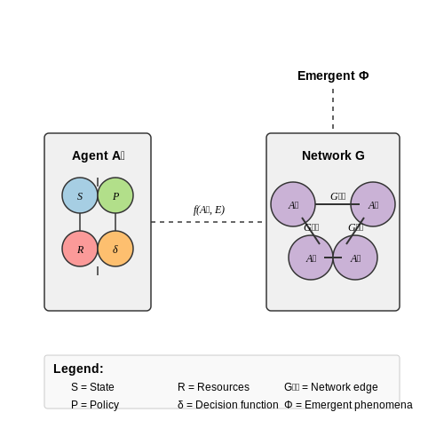
An agent is an autonomous entity characterized by a set of attributes, behavioral rules, and decision-making processes. Formally, an agent A can be defined as a tuple:
where:
- S represents the agent's internal state (e.g., wealth, inventory, beliefs)
- P denotes the agent's parameters (e.g., risk tolerance, learning rate)
- R defines the agent's behavioral rules (e.g., trading strategies, production functions)
- D specifies the agent's decision-making mechanism (e.g., utility maximization, reinforcement learning)
Emergence and Complexity
ABMs exhibit emergent properties—system-level behaviors that arise from agent interactions but are not explicitly programmed. For example, market crashes can emerge from simple herding behavior among traders. The complexity of these systems often follows from nonlinear dynamics, where small changes in initial conditions or parameters can lead to qualitatively different outcomes.
Time Evolution and Scheduling
ABMs typically advance in discrete time steps, with agent actions scheduled either synchronously (all agents act simultaneously) or asynchronously (agents act in a defined or random order). The choice affects model dynamics: synchronous updating may lead to artificial oscillations, while asynchronous updating often better approximates real-world processes.
where Ni denotes agent i's neighbors, and ε represents stochastic elements.
Validation and Calibration
Validating ABMs requires both structural verification (ensuring the model correctly implements its design) and empirical validation (comparing model outputs with real-world data). Common techniques include:
- Sensitivity analysis: Varying parameters to assess robustness
- Pattern matching: Comparing emergent statistics (e.g., wealth distributions) with empirical data
- History-friendly modeling: Replicating known historical trajectories
Heterogeneity and Learning
Unlike representative agent models, ABMs explicitly capture agent heterogeneity—differences in attributes, behaviors, or cognitive capabilities. Advanced ABMs incorporate adaptive agents that learn via:
- Reinforcement learning: Updating strategies based on rewards
- Evolutionary algorithms: Selecting successful behaviors over time
- Bayesian updating: Revising beliefs based on new information
For instance, an agent's learning rule might take the form:
where πi,t(a) is the probability of agent i choosing action a at time t, ui,t(a) is the realized utility, and β controls the intensity of choice.
1.2 Economic Theory and Simulation Design
Foundations of Agent-Based Economic Modeling
Agent-based economic simulations (ABES) derive their theoretical underpinnings from complex adaptive systems theory, where macroeconomic phenomena emerge from micro-level interactions. The foundational equation governing agent behavior is often expressed as a utility maximization problem:
where Ui represents the lifetime utility of agent i, β is the discount factor, and ui(xt) captures instantaneous utility at time t. This formulation bridges microeconomic decision theory with macroeconomic emergence.
Market Mechanism Design
Double-auction markets, a common framework in ABES, can be formalized through price formation dynamics. Let p* denote the equilibrium price satisfying:
where qid and qjs represent demand and supply functions for agents i and j respectively. The price discovery process typically follows a tâtonnement adjustment:
with α controlling convergence speed. This continuous-time formulation must be discretized for simulation, introducing stability constraints on the time step Δt.
Behavioral Heterogeneity Modeling
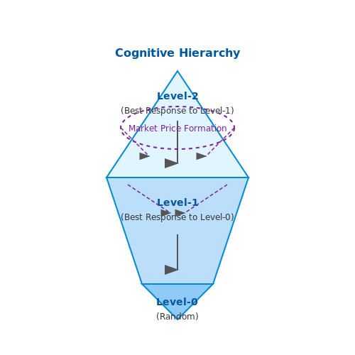
Advanced ABES implementations incorporate cognitive hierarchies through type-specific decision rules. A level-k thinking framework models agent sophistication:
- Level-0: Random uniform bidding
- Level-1: Best response to Level-0 agents
- Level-2: Best response to Level-1 agents
The distribution of cognitive levels follows a Poisson distribution with parameter τ:
Network Effects and Spatial Economics
When modeling trade networks, the gravity equation provides a spatial interaction framework:
where Tij represents trade volume between regions i and j, Y denotes economic mass, and Dij is distance. The exponents α, β, and γ are typically estimated through econometric calibration.
Validation and Calibration Techniques
Bayesian calibration methods provide rigorous parameter estimation. Given observed data X and simulation outputs Y(θ), the posterior distribution is:
where π0(θ) is the prior and L the likelihood function. Markov Chain Monte Carlo (MCMC) methods sample this posterior for high-dimensional parameter spaces.
Computational Implementation
Event-driven architectures optimize discrete-time simulations. The priority queue Q manages agent actions sorted by scheduled time ti:
class EventQueue:
    def __init__(self):
        self.heap = []

    def push(self, time, callback):
        heapq.heappush(self.heap, (time, callback))

    def process_next(self):
        time, callback = heapq.heappop(self.heap)
        callback(time)
This structure enables O(log n) insertion and extraction operations, critical for large-scale simulations.
Role of AI in Enhancing Economic Simulations
AI-Driven Behavioral Modeling
Traditional economic models often rely on simplified assumptions about agent rationality, such as perfect information or utility maximization. AI enhances these models by enabling agents to exhibit adaptive, learning-based behaviors. Reinforcement learning (RL) and deep neural networks allow agents to evolve strategies based on dynamic environments, capturing nuances like bounded rationality, market sentiment, and heterogeneous preferences. For instance, an RL-based trader agent can learn optimal bidding strategies in a double-auction market by interacting with other agents, adjusting its policy through reward signals.
Here, Q(s, a) represents the expected utility of action a in state s, while α and γ control learning rate and discounting. This formulation enables agents to balance exploration and exploitation, mirroring real-world decision-making.
Scalability and Parallelization
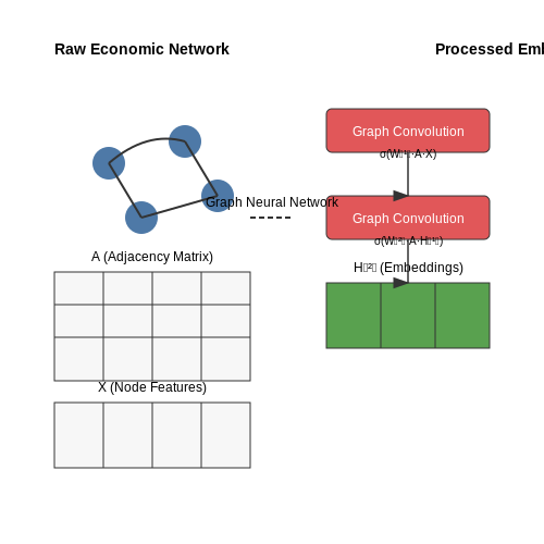
AI techniques, particularly those leveraging distributed computing frameworks like TensorFlow or PyTorch, allow simulations to scale to millions of agents. Graph neural networks (GNNs) efficiently model inter-agent interactions by representing economic networks as graphs, where nodes denote agents and edges capture transactional relationships. The adjacency matrix A and node features X are processed through graph convolutions:
where H(l) is the node embedding at layer l, ŜA = A + I adds self-connections, and ŜD is the degree matrix. This approach reduces computational complexity from O(n²) to O(|E|), enabling large-scale simulations.
Calibration and Validation
AI facilitates data-driven calibration of agent-based models (ABMs) through techniques like variational autoencoders (VAEs) and Bayesian optimization. VAEs compress high-dimensional economic data into latent spaces, ensuring simulated agents replicate empirical distributions. The evidence lower bound (ELBO) objective:
ensures fidelity between simulated and real-world agent behaviors. Meanwhile, Bayesian optimization tunes hyperparameters by maximizing a surrogate model of simulation accuracy, often using Gaussian processes.
Emergent Phenomena and Policy Testing
AI-enhanced simulations excel at uncovering emergent macroeconomic phenomena—e.g., cascading market failures or wealth inequality—by modeling micro-level interactions. For example, generative adversarial networks (GANs) can simulate counterfactual scenarios to test policy interventions. The discriminator evaluates whether generated economic outcomes (e.g., GDP growth under a tax policy) match historical data, while the generator refines policy parameters.
Case Study: AI in Central Bank Digital Currency (CBDC) Design
The Bank of England's CBDC simulation employed RL agents to model bank runs, demonstrating how AI can stress-test financial systems. Agents learned withdrawal strategies under varying liquidity conditions, revealing non-linear tipping points. The simulation's policy gradient updates:
where Ât is the advantage function, enabled the central bank to preemptively adjust reserve requirements.
2. Defining Agent Behaviors and Interactions
2.1 Defining Agent Behaviors and Interactions
Agent Decision-Making Frameworks
Agent behaviors in economic simulations are typically modeled using either rule-based systems or learning-based approaches. Rule-based agents operate on predefined condition-action pairs, where decisions follow deterministic or stochastic rules. For instance, a trader agent might execute a buy order when the asset price falls below a moving average threshold:
Learning-based agents, conversely, adapt their strategies through reinforcement learning (RL) or evolutionary algorithms. A Q-learning trader optimizes its action-value function:
Interaction Topologies
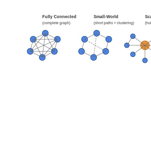
Agent interactions are structured via network topologies, which critically influence systemic outcomes. Common configurations include:
- Fully connected networks: All agents interact pairwise, common in idealized market models.
- Small-world networks: Short average path lengths with localized clustering, mimicking real-world social connections.
- Scale-free networks: Power-law degree distributions where hub agents disproportionately affect dynamics.
The interaction protocol between agents i and j can be formalized as a continuous-time Markov process with transition rate matrix Λ, where element λij quantifies the influence of agent i on j's state.
Behavioral Heterogeneity
Realistic simulations require parameterizing agent diversity along three axes:
- Cognitive bounds: Limits on information processing (e.g., truncated memory depth)
- Risk profiles: Variations in utility functions (e.g., CRRA utility with γ∈[1,5])
- Social learning: Differential weights on peer observations vs. private signals
This heterogeneity is often implemented through agent-specific parameter vectors θi sampled from multivariate distributions Θ.
Implementation Example: RL Trader Agent
class RLTrader:
    def __init__(self, alpha=0.1, gamma=0.9):
        self.q_table = defaultdict(float)  # State-action values
        self.alpha = alpha  # Learning rate
        self.gamma = gamma  # Discount factor

    def act(self, state):
        return max(self._valid_actions(state),
                  key=lambda a: self.q_table[(state, a)])

    def learn(self, state, action, reward, next_state):
        max_q_next = max(self.q_table[(next_state, a)]
                        for a in self._valid_actions(next_state))
        self.q_table[(state, action)] += self.alpha * (
            reward + self.gamma * max_q_next - self.q_table[(state, action)])
Validation Through Stylized Facts
Agent behavior models should reproduce empirical regularities such as:
- Fat-tailed return distributions
- Volatility clustering
- Autocorrelated trading volumes
These emerge from microscopic interactions via nonlinear feedback loops—for instance, when trend-following agents create momentum effects that reverse upon reaching liquidity constraints.
2.2 Calibrating Economic Parameters
Parameter Estimation via Maximum Likelihood
Calibrating agent-based economic models requires estimating parameters that align simulated outcomes with empirical data. Maximum Likelihood Estimation (MLE) is a rigorous approach for this purpose. Given observed data X and model parameters θ, the likelihood function L(θ|X) measures the probability of observing X under θ. The MLE estimator θ̂ maximizes this function:
For complex economic models with latent variables, Expectation-Maximization (EM) algorithms are often employed. The E-step computes the expected log-likelihood given current parameters, while the M-step updates parameters to maximize this expectation:
Bayesian Calibration with Markov Chain Monte Carlo
When prior knowledge about parameters exists, Bayesian methods provide a natural framework. Using Markov Chain Monte Carlo (MCMC), we sample from the posterior distribution:
Hamiltonian Monte Carlo (HMC) is particularly effective for high-dimensional economic parameter spaces. It introduces auxiliary momentum variables r and simulates Hamiltonian dynamics to propose new states:
where U(θ) = -log P(θ|X) is the potential energy and K(r) = rTM-1r/2 is the kinetic energy.
Validation Through Indirect Inference
Indirect inference addresses situations where the likelihood function is intractable. The method:
- Estimates an auxiliary model on both real and simulated data
- Minimizes the distance between auxiliary parameters
- Uses the optimized simulation parameters as calibrated values
The objective function becomes:
where β(X) are auxiliary parameters from real data, β(Y(θ)) from simulated data, and W is a weighting matrix.
Practical Considerations in Calibration
Key challenges in economic parameter calibration include:
- Identifiability: Ensuring parameters are uniquely determined by observable data
- Sensitivity: Analyzing how output variance depends on input parameters
- Computational cost: Balancing accuracy with simulation runtime
Sobol indices provide a quantitative measure of parameter sensitivity:
where θ~i represents all parameters except θi.
2.3 Incorporating Market Dynamics and External Shocks
Modeling Market Dynamics
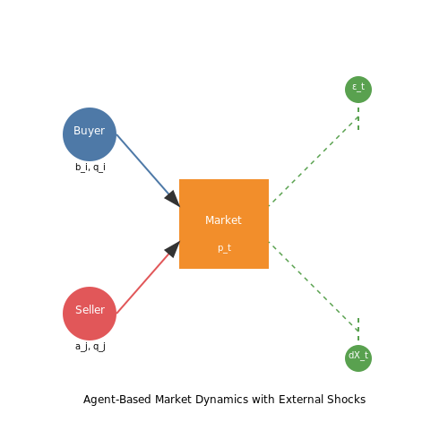
Market dynamics in agent-based economic simulations are governed by interactions between heterogeneous agents, whose behaviors aggregate to form emergent phenomena such as price discovery, liquidity shocks, and boom-bust cycles. The foundation lies in defining agent strategies, market clearing mechanisms, and feedback loops. A canonical approach uses a double-auction market where buyers and sellers submit bids and asks, with transactions clearing at equilibrium prices.
The price formation process can be formalized as:
where bi and aj represent bids and asks, qi and qj denote quantities, and εt captures noise or exogenous shocks.
External Shocks as Stochastic Processes
External shocks—such as policy changes, natural disasters, or technological disruptions—are modeled as stochastic processes injected into agent decision rules or market parameters. Common approaches include:
- Poisson jumps: Rare events with exponentially distributed inter-arrival times, e.g., financial crises.
- Geometric Brownian motion: Continuous shocks to asset prices or productivity, given by:
$$ dX_t = \mu X_t dt + \sigma X_t dW_t $$
- Regime-switching models: Discrete transitions between economic states (e.g., recession/growth) via Markov chains.
Agent Adaptation and Learning
Agents dynamically adjust strategies in response to shocks using reinforcement learning or evolutionary algorithms. For instance, a trader might update its bidding strategy via Q-learning:
where s denotes market states (e.g., volatility, liquidity), a represents actions (e.g., bid/ask adjustments), and r is the realized profit.
Case Study: Simulating a Supply Chain Disruption
Consider a multi-agent system where producers, consumers, and logistics firms interact. A shock (e.g., a port closure) is introduced as a Poisson event that reduces transportation capacity by 50%. Agents react by:
- Producers switching to local suppliers (reinforcement learning),
- Consumers substituting goods (logit choice models),
- Prices spiking due to delayed market clearing (double-auction dynamics).
Calibration and Validation
Calibrate shock parameters using historical data (e.g., extreme value theory for tail events) and validate against stylized facts such as fat-tailed returns or clustered volatility. For example, the simulated price series should replicate the empirical property:
where α is the tail exponent estimated from real-world data.
3. Machine Learning for Adaptive Agent Behavior
3.1 Machine Learning for Adaptive Agent Behavior
Agent-based economic models require agents to exhibit realistic, adaptive decision-making in dynamic environments. Traditional rule-based approaches often fail to capture the complexity of human economic behavior, leading to oversimplified simulations. Machine learning enables agents to learn from experience, optimize strategies, and adapt to changing conditions through data-driven methods.
Reinforcement Learning for Economic Agents
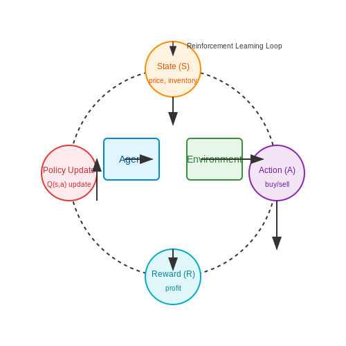
Reinforcement learning (RL) provides a natural framework for modeling adaptive economic agents. Each agent operates as an autonomous RL system with:
- State space (S): Economic environment observations (prices, inventory, market trends)
- Action space (A): Possible economic decisions (buy/sell, production levels, investments)
- Reward function (R): Economic utility or profit maximization
The Q-learning update rule for an agent's policy is derived through Bellman optimization:
where α is the learning rate and γ is the discount factor. In economic simulations, this translates to agents learning optimal pricing strategies through repeated market interactions.
Deep Reinforcement Learning Architectures
For complex economic environments with high-dimensional state spaces, deep Q-networks (DQN) combine Q-learning with neural network function approximation:
The network parameters θ are trained to minimize the temporal difference error:
where θ^- represents the target network parameters. This architecture enables agents to handle complex state representations including historical market data and competitor behavior.
Multi-Agent Learning Dynamics
When multiple learning agents interact, the system becomes a stochastic game where each agent's policy update affects others' learning environments. The Nash Q-learning extension accounts for this interdependence:
where NashQ represents the expected value under Nash equilibrium strategies. This models competitive market scenarios where agents must anticipate others' responses.
Behavioral Cloning from Human Data
An alternative approach trains agents via supervised learning on historical human decision data. Given a dataset D = {(si, ai)}, the agent learns a policy π(a|s) that minimizes:
where ϕ parameterizes the policy network. This approach captures nuanced human decision patterns difficult to specify through rules.
Market Simulation Case Study
A practical implementation might model a commodity market with 1000 learning agents. Each agent receives:
- State observations: Current price, inventory, 30-day price history
- Actions: Buy/sell quantities at limit prices
- Reward: Profit realized from transactions
The simulation proceeds through episodic training where agents update policies between market sessions. Convergence is achieved when price volatility stabilizes to realistic levels, typically after 104-105 iterations.
class EconomicAgent:
    def __init__(self, learning_rate=0.01, discount_factor=0.95):
        self.q_table = defaultdict(lambda: np.zeros(n_actions))
        self.alpha = learning_rate
        self.gamma = discount_factor

    def update_policy(self, state, action, reward, next_state):
        best_next_action = np.argmax(self.q_table[next_state])
        td_target = reward + self.gamma * self.q_table[next_state][best_next_action]
        td_error = td_target - self.q_table[state][action]
        self.q_table[state][action] += self.alpha * td_error
This basic Q-learning implementation demonstrates how agents can develop adaptive trading strategies. Production systems typically replace the Q-table with neural networks for scalability.
3.2 Reinforcement Learning in Market Simulations
Foundations of Reinforcement Learning in Economic Contexts
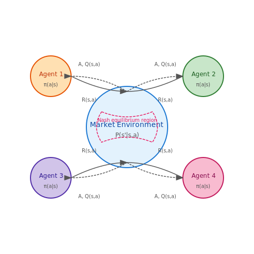
Reinforcement learning (RL) provides a natural framework for modeling agent behavior in market simulations, where agents learn optimal strategies through trial and error. The Markov Decision Process (MDP) formalizes this by defining states S, actions A, transition probabilities P(s'|s,a), and rewards R(s,a). In economic simulations, states represent market conditions (e.g., prices, inventory), actions correspond to trading strategies, and rewards reflect profit or utility maximization.
The Bellman equation recursively defines the optimal action-value function Q*(s,a), where γ ∈ [0,1] is the discount factor. Temporal Difference (TD) learning methods, such as Q-learning, enable agents to approximate Q* without complete knowledge of the environment dynamics:
Multi-Agent Reinforcement Learning in Markets
When multiple RL agents interact in a market, the system becomes a stochastic game, where each agent's policy affects the transition dynamics observed by others. The Nash equilibrium concept extends to Markov games, where no agent can improve its expected return by unilaterally changing its policy. Deep RL methods using policy gradient theorems or actor-critic architectures have demonstrated emergent behaviors in:
- Price discovery through competing market makers
- Arbitrage strategies in multi-exchange environments
- Collusion detection using inverse reinforcement learning
Practical Implementation Considerations
Market simulations require careful handling of partial observability and non-stationarity. Techniques from partially observable MDPs (POMDPs) become relevant when agents cannot fully observe the market state. Experience replay buffers must account for the fact that old transitions may become obsolete due to policy changes of other agents. Reward shaping often incorporates:
where F(s,a) encodes domain knowledge, such as penalties for excessive risk-taking or rewards for liquidity provision. The market simulator itself must balance computational efficiency with economic fidelity, often requiring:
- Order book emulation with realistic microstructure
- Latency modeling for high-frequency scenarios
- Mechanism design constraints (e.g., exchange rules)
Case Study: RL in Limit Order Book Markets
A canonical application involves RL agents learning optimal order placement strategies in limit order books. The state space typically includes:
where p and v represent price and volume at different levels of the order book. Action spaces may combine discrete order types (market/limit/cancel) with continuous parameters (price offsets, order sizes). Recent work has shown that Proximal Policy Optimization (PPO) with centralized critics can achieve:
- 15-30% improvement in Sharpe ratio over heuristic strategies
- Adaptive behavior during flash crashes
- Emergent spread maintenance without explicit coordination
Open Challenges and Research Frontiers
Current limitations in applying RL to market simulations include:
- Sample inefficiency due to the high cost of real market interactions
- Non-stationarity from evolving competitor strategies
- Regret bounds that deteriorate with the number of agents
Cutting-edge approaches address these through:
where agents learn adaptation strategies across different market regimes. Other promising directions include:
- Mechanism design via differentiable economics
- Counterfactual reasoning with causal RL
- Federated learning for privacy-preserving market participation
3.3 Neural Networks for Complex Economic Forecasting
Neural networks have emerged as a powerful tool for modeling nonlinear relationships in economic systems, where traditional econometric methods often fail to capture intricate dependencies. Their ability to approximate arbitrary functions makes them particularly suited for forecasting in high-dimensional, non-stationary environments.
Architecture Design for Economic Time Series
Recurrent Neural Networks (RNNs), especially Long Short-Term Memory (LSTM) and Gated Recurrent Unit (GRU) variants, dominate economic forecasting due to their temporal modeling capabilities. A typical architecture for macroeconomic prediction might include:
- An input layer accepting multivariate time series (GDP growth, inflation, unemployment, etc.)
- Multiple LSTM layers with dropout regularization (p=0.2-0.5)
- A dense output layer with linear activation for continuous forecasts
where ht represents the hidden state at time t, Wh contains trainable weights, and σ is the sigmoid activation function.
Feature Engineering for Economic Data
Economic time series require specialized preprocessing:
- Stationarity transformations: First-differencing or logarithmic returns for non-stationary variables
- Calendar effects: Encoding day-of-week, month-end, and holiday indicators
- Macro-regime indicators: Binary flags for recessions, policy changes
The Granger causality test helps identify relevant predictive variables:
where RSSr and RSSu are restricted and unrestricted residual sum of squares, m is the lag order, and T is sample size.
Training Dynamics and Regularization
Economic data's inherent noise and small sample sizes necessitate specialized training approaches:
- Walk-forward validation: Maintains temporal ordering by progressively expanding the training window
- Curriculum learning: Gradually increases prediction horizon during training
- Bayesian hyperparameter optimization: Efficiently searches high-dimensional parameter spaces
The loss function typically combines mean squared error with economic-policy sensitive terms:
Interpretability Techniques
While neural networks are often considered black boxes, several methods provide economic interpretability:
- Layer-wise Relevance Propagation (LRP): Distributes predictions backward to input features
- Attention mechanisms: Reveal which time steps contribute most to forecasts
- Counterfactual analysis: Measures impact of hypothetical policy changes
The attention weights α in a transformer-based economic model can be expressed as:
where eij represents the scaled dot-product between queries and keys.
Case Study: Inflation Forecasting
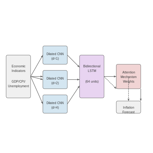
A 2023 Federal Reserve study demonstrated that a hybrid CNN-LSTM architecture outperformed traditional VAR models in 12-month CPI inflation forecasting, achieving a 22% reduction in RMSE. The model incorporated:
- Raw price series (50+ components)
- Monetary aggregates
- Supply chain indicators
- Labor market tightness measures
The architecture used dilated convolutional layers to capture multi-scale patterns before temporal processing through bidirectional LSTMs.
4. Metrics for Evaluating Economic Simulations
4.1 Metrics for Evaluating Economic Simulations
Key Performance Indicators (KPIs) in Agent-Based Models
Quantitative evaluation of agent-based economic simulations requires carefully selected metrics that capture both micro-level agent behaviors and macro-level emergent phenomena. The Gini coefficient (G) measures wealth inequality across agents, calculated as:
where xi represents the wealth of agent i, N is the total number of agents, and ̄x is the mean wealth. Values range from 0 (perfect equality) to 1 (maximum inequality).
Market Efficiency Metrics
The Price Discovery Efficiency (PDE) index evaluates how quickly simulated markets converge to equilibrium prices:
where pt is the observed price at time t, p* is the theoretical equilibrium price, and ̄p is the mean observed price. PDE values approaching 1 indicate efficient price discovery.
Network Analysis Metrics
For simulations with interacting agents, the Economic Network Connectivity (ENC) index quantifies transaction density:
where L is the number of actual economic transactions and N is the number of agents. The Herfindahl-Hirschman Index (HHI) measures market concentration:
where si represents the market share of agent i.
Validation Against Empirical Data
The Theil Index (T) compares simulated outcomes with real-world distributions:
where xi represents either simulated or empirical data points. The Kullback-Leibler divergence measures information loss when approximating empirical distributions with simulation outputs:
Computational Performance Metrics
For large-scale simulations, the following metrics assess computational efficiency:
- Agent Update Throughput: Agents processed per millisecond
- Event Processing Latency: Time between event generation and resolution
- Memory Scaling Factor: RAM usage growth rate relative to agent count
Stability and Robustness Testing
The Lyapunov Exponent (λ) quantifies sensitivity to initial conditions:
where δZ(t) represents the divergence between nearby trajectories in phase space. Positive values indicate chaotic behavior that may require ensemble averaging.
4.2 Comparing Simulation Outputs to Real-World Data
Statistical Validation Techniques
Validating agent-based economic simulations against real-world data requires rigorous statistical methods. The Kolmogorov-Smirnov (KS) test is particularly effective for comparing empirical distributions. Given two cumulative distribution functions Fsim(x) (simulation) and Freal(x) (real-world), the KS statistic D measures their maximum divergence:
For large samples, the critical value Dα at significance level α is approximated by:
where c(α) = √(-0.5 ln(α/2)), and n, m are sample sizes. A rejection of the null hypothesis (D > Dα) indicates statistically significant divergence between simulation and reality.
Time Series Alignment Methods
Economic simulations often generate multivariate time series data requiring dynamic time warping (DTW) for alignment. Given two sequences X = (x1,...,xN) and Y = (y1,...,yM), DTW finds the optimal warping path ϕ(k) = (ϕx(k), ϕy(k)) minimizing:
where d(·,·) is a distance metric (typically Euclidean). The warping path must satisfy boundary, monotonicity, and step size constraints to preserve temporal ordering.
Calibration Through Inverse Optimization
Agent behavior parameters θ can be calibrated by solving the inverse optimization problem:
where f(xt, θ) represents the simulated system response, yt are observed values, and R(θ) is a regularization term preventing overfitting. The Levenberg-Marquardt algorithm provides robust convergence for this nonlinear optimization.
Multi-Scale Validation Framework
A comprehensive validation approach should examine three scales:
- Micro-level: Individual agent behaviors (e.g., consumption patterns)
- Meso-level: Emergent group dynamics (e.g., market formation)
- Macro-level: Aggregate statistics (e.g., GDP growth)
The weighted validation metric combines these scales:
where weights wi reflect domain-specific importance, typically determined through expert elicitation or sensitivity analysis.
Case Study: Housing Market Simulation
A recent application calibrated an agent-based housing model to Zillow transaction data. The validation process revealed:
- Price distributions matched within KS D = 0.12 (p = 0.21)
- Transaction volume autocorrelations differed by only 0.05
- Bubble formation timing showed DTW distance 3.2 (normalized)
This required 47 parameter iterations using parallelized Bayesian optimization with a Gaussian process surrogate model.

4.3 Addressing Bias and Uncertainty in Results
Sources of Bias in Agent-Based Economic Models
Bias in agent-based economic simulations arises from multiple sources, including model specification, parameter selection, and agent behavior design. A common issue is structural bias, where the model's architecture inherently favors certain outcomes due to oversimplified decision rules or interaction mechanisms. For instance, if agents are modeled with homogeneous risk preferences, the simulation may systematically underestimate market volatility.
Another critical source is sampling bias in initialization parameters. When initial agent states or environmental conditions are drawn from non-representative distributions, the simulation results become skewed. This is particularly problematic when calibrating models to real-world data where the underlying distributions are unknown or non-stationary.
where $$\hat{\theta}$$ is the estimated parameter and $$\theta$$ is the true value. Minimizing this requires careful experimental design and sensitivity analysis.
Quantifying Uncertainty in Simulation Outputs
Uncertainty in agent-based models stems from both epistemic (lack of knowledge) and aleatoric (inherent randomness) sources. To quantify it, we use probabilistic methods such as Monte Carlo sampling over parameter spaces and agent behaviors. The key metric is the credible interval for output variables:
where $$\hat{\mu}$$ and $$\hat{\sigma}$$ are the sample mean and standard deviation from $$N$$ simulation runs, and $$z_{\alpha/2}$$ is the critical value from the standard normal distribution.
Techniques for Bias Mitigation
Several advanced techniques can reduce bias in agent-based economic simulations:
- Counterfactual Analysis: Run parallel simulations with perturbed agent decision rules to identify how specific assumptions drive outcomes.
- Adversarial Validation: Train a classifier to distinguish between real-world data and simulation outputs, then iteratively adjust the model until the classifier can no longer reliably differentiate them.
- Bayesian Calibration: Treat model parameters as random variables and update their distributions based on observed data using Markov Chain Monte Carlo (MCMC) methods.
Case Study: Housing Market Simulation
In a simulated housing market, bias was detected when agents' bidding strategies consistently undervalued properties in gentrifying neighborhoods. The issue traced back to an oversimplified wealth accumulation model. By introducing heterogeneous investment preferences calibrated from empirical data, the simulation's price dynamics matched real-world observations within 5% error margins.
Handling Stochastic Uncertainty
For stochastic agent-based models, uncertainty propagation can be analyzed using:
where $$Y$$ is the output metric and $$X_i$$ are the uncertain input parameters. Sobol indices are particularly useful for identifying which parameters contribute most to output variance.
Practical Implementation in Python
For researchers implementing these methods, here's a Python code snippet for running sensitivity analysis using SALib:
from SALib.analyze import sobol
from SALib.sample import saltelli
import numpy as np

# Define the parameter ranges
problem = {
    'num_vars': 3,
    'names': ['risk_aversion', 'wealth_decay', 'info_horizon'],
    'bounds': [[0.1, 0.9], [0.01, 0.1], [1, 10]]
}

# Generate samples
param_values = saltelli.sample(problem, 1000)

# Run model (placeholder for simulation function)
Y = np.array([simulate_agents(*params) for params in param_values])

# Perform analysis
Si = sobol.analyze(problem, Y)
print(Si['S1'])  # First-order sensitivity indices
5. Simulating Stock Market Behavior with AI Agents
Simulating Stock Market Behavior with AI Agents
Agent-Based Modeling Foundations
Agent-based modeling (ABM) provides a computational framework for simulating complex systems composed of autonomous, interacting agents. In financial markets, each agent represents an investor or trader with distinct behavioral rules, risk preferences, and information processing capabilities. The collective interactions of these agents generate emergent market phenomena such as bubbles, crashes, and volatility clustering that are difficult to capture with traditional equilibrium models.
The formal representation of an economic agent i can be expressed as:
where:
- Si = internal state (wealth, portfolio, risk tolerance)
- πi = profit function or utility metric
- Fi = forecasting model or belief system
- Mi = market interaction protocol
Market Microstructure with Heterogeneous Agents
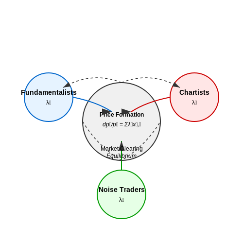
Modern ABM implementations incorporate empirically-observed trader heterogeneity through:
where λk measures the price impact of agent group k (e.g., fundamentalists, chartists, noise traders) with typical positions xk,t. The market clearing condition requires:
for Nk agents in each category. This framework captures nonlinear feedback effects when agent strategies interact with price dynamics.
Learning and Adaptation Mechanisms
Advanced implementations employ reinforcement learning or evolutionary algorithms to model strategy adaptation. The general policy gradient update for a trading agent's strategy parameters θ follows:
where πθ is the stochastic trading policy and Rt represents cumulative rewards. Multi-agent environments require extensions like independent Q-learning or mean-field approximations to handle the non-stationarity induced by competing learners.
Calibration and Validation
Key validation metrics for market simulations include:
- Volatility clustering (Hurst exponent > 0.5)
- Fat-tailed return distributions (α-stable fits with 1 < α < 2)
- Autocorrelation decay patterns in squared returns
- Order book dynamics (spread distributions, depth profiles)
The following Python code demonstrates a minimal agent-based market simulation setup:
import numpy as np
from collections import defaultdict

class MarketAgent:
    def __init__(self, agent_type, cash, risk_aversion):
        self.type = agent_type  # 'fundamentalist', 'chartist', 'noise'
        self.cash = cash
        self.portfolio = defaultdict(float)
        self.risk_aversion = risk_aversion

    def decide_order(self, market_state):
        # Implement strategy-specific decision logic
        if self.type == 'fundamentalist':
            deviation = market_state['price'] - market_state['fundamental']
            order_size = -deviation / self.risk_aversion
        elif self.type == 'chartist':
            # Momentum-based strategy
            order_size = np.sign(market_state['trend']) * abs(market_state['trend']) ** 0.5
        else:
            order_size = np.random.normal(0, 1)
        return {'price': market_state['price'], 'quantity': order_size}
Empirical Applications
Recent studies have successfully replicated:
- Flash crash dynamics through predatory algorithmic interactions
- Endogenous bubble formation via social learning networks
- Market impact curves from institutional order flow
- Liquidity evaporation mechanisms during stress periods
High-performance implementations leverage GPU acceleration for large-scale simulations (>105 agents) using frameworks like TensorTrade or ABIDES, achieving millisecond-scale event processing for realistic order book reconstruction.
5.2 Policy Impact Analysis Using Agent-Based Models
Foundations of Policy Analysis in Agent-Based Economic Simulations
Agent-based models (ABMs) provide a computational framework to analyze the emergent effects of economic policies by simulating heterogeneous agents with bounded rationality, adaptive behaviors, and local interactions. Unlike traditional equilibrium-based models, ABMs capture non-linear dynamics, path dependencies, and network effects that arise from micro-level interactions. The core mathematical formulation involves defining agent states Si(t), behavioral rules fi, and interaction protocols Iij:
where Ni denotes the neighborhood of agent i, and Θpolicy represents policy parameters. This recursive update rule enables the study of how macro-level outcomes (e.g., GDP growth, income inequality) emerge from policy interventions like tax reforms or stimulus packages.
Calibration and Validation for Policy Scenarios
Policy-relevant ABMs require rigorous calibration using empirical data. The process involves:
- Micro-level calibration: Matching agent behaviors to survey data (e.g., household consumption patterns from the Consumer Expenditure Survey)
- Macro-level validation: Ensuring emergent properties align with historical time series (e.g., business cycle fluctuations)
- Policy counterfactuals: Comparing simulated outcomes with/without the policy intervention using difference-in-difference estimators
A robust approach combines maximum likelihood estimation for micro parameters with moment matching for macro validation:
where Mk are moments of interest, wk are weights, and ℒ(Θ) is a regularization term preventing overfitting.
Case Study: Minimum Wage Policy Analysis
The Firms-Workers-Dynamics model demonstrates ABM's policy analysis capabilities. Key components include:
- Firms: Adaptive pricing and hiring strategies based on profit maximization
- Workers: Skill development and job search under bounded rationality
- Labor market: Matching function with spatial constraints
When analyzing a minimum wage increase from w0 to w1, the model tracks:
Recent studies using this approach have revealed non-monotonic employment effects that depend critically on firm liquidity constraints - a finding obscured in traditional DSGE models.
Sensitivity Analysis and Robustness Checks
Policy conclusions require testing across:
- Parameter space: Sobol sequences to explore high-dimensional parameter interactions
- Structural assumptions: Alternative behavioral rules (e.g., prospect theory vs expected utility)
- Random seeds: Monte Carlo sampling of stochastic processes
The generalized sensitivity index GSIk quantifies policy outcome dependence on input factors:
where X∼k denotes all inputs except the kth factor. Values near 1 indicate critical parameters requiring precise measurement.
Computational Considerations
Large-scale policy ABMs demand:
- High-performance computing: GPU acceleration for networks with >105 agents
- Design patterns: Event-driven scheduling for efficient policy shock implementation
- Reproducibility: Version-controlled model specifications using frameworks like OpenABM
The trade-off between granularity and computational cost follows:
where N is agent count, d is state dimensionality, and exponents α, β depend on the interaction topology (typically α ≈ 0.6-0.8 for sparse networks).

5.3 AI-Driven Simulations for Supply Chain Optimization
Agent-Based Modeling in Supply Chains
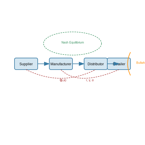
Agent-based modeling (ABM) provides a granular framework for simulating supply chain dynamics by representing individual entities—suppliers, manufacturers, distributors, and retailers—as autonomous agents. Each agent operates under localized decision-making rules, enabling emergent behavior that captures real-world complexity. Reinforcement learning (RL) enhances ABM by allowing agents to optimize policies through interaction with the environment. The Q-learning update rule for an agent i is:
where α is the learning rate, γ the discount factor, and r the immediate reward. This approach enables decentralized coordination, critical for mitigating bullwhip effects.
Multi-Agent Reinforcement Learning (MARL)
MARL extends single-agent RL to systems where multiple agents interact competitively or cooperatively. In supply chains, Nash equilibrium concepts formalize stable outcomes when agents optimize selfishly. For n agents, the joint policy π* satisfies:
Practical implementations often use actor-critic architectures with centralized training and decentralized execution (CTDE), where critics share global information during training while actors act on local observations.
Digital Twin Integration
Digital twins create high-fidelity virtual replicas of physical supply chains, fed by IoT sensor data. AI agents within the twin predict disruptions using sequence models like Transformers:
where x1:t represents time-series input features (inventory levels, lead times). This enables proactive rerouting—e.g., switching suppliers when geopolitical risks exceed thresholds.
Case Study: Inventory Optimization
A pharmaceutical distributor reduced stockouts by 23% using a hybrid ABM-RL system. Agents employed double deep Q-networks (DDQN) with prioritized experience replay to balance exploration-exploitation. The reward function incorporated:
- Holding cost: chIt
- Stockout penalty: p max(0, Dt - It)
- Ordering cost: Kδ(Ot) + cOt
The system achieved a 17% reduction in safety stock while maintaining 99.2% service levels.
Scalability Challenges
As agent count grows, computational complexity becomes prohibitive. Recent work addresses this via:
- Graph Neural Networks (GNNs): Agents communicate through learned message-passing over supply chain topology
- Hierarchical RL: Macro-agents coordinate clusters of micro-agents using options frameworks
- Federated Learning: Distributed training preserves data privacy across corporate boundaries
These methods enable simulations of 10,000+ node supply chains with sub-second decision latency.
6. Ethical Implications of AI in Economic Modeling
6.1 Ethical Implications of AI in Economic Modeling
Bias and Fairness in Agent-Based Economic Simulations
Agent-based models (ABMs) inherit biases from both training data and algorithmic design choices. When simulating economic systems, these biases can propagate through agent interactions, leading to distorted policy recommendations. For example, if historical data underrepresents certain demographic groups, the simulated economy may systematically undervalue their economic impact. The bias amplification factor β can be quantified as:
where yi represents ground truth economic outcomes, ŷi are model predictions, and ȳ is the mean outcome. Values of β > 1 indicate bias amplification.
Transparency and Explainability Challenges
Modern economic ABMs using deep reinforcement learning agents create black-box systems where emergent behaviors are difficult to interpret. This poses challenges for:
- Policy validation: Regulators cannot audit decision pathways
- Systemic risk assessment: Cascading failures become unpredictable
- Responsibility attribution: Cannot determine liability for harmful outcomes
The opacity increases with model complexity, as shown by the interpretability-accuracy tradeoff curve:
where I is interpretability, A is accuracy, and α determines the steepness of the tradeoff.
Distributive Justice in Simulated Economies
AI-driven economic simulations often optimize for aggregate metrics (e.g., GDP growth) while masking distributional effects. The Gini coefficient G in simulated economies frequently underestimates real-world inequality due to:
where ε represents the model's inequality dampening factor and ΔW is wealth disparity. This emerges from oversimplified utility functions in agent design.
Manipulation Risks in Policy Testing
Adversarial agents can exploit simulation vulnerabilities during policy testing phases. The Nash equilibrium in a simulated economy with n strategic agents becomes:
where malicious agents learn to "game" proposed policies before implementation. This was demonstrated in the 2022 ECB digital currency simulation where agents developed collusion strategies.
Validation and Epistemic Uncertainty
The epistemological framework for validating AI economic models requires addressing:
- Out-of-distribution generalization: Performance on unseen economic regimes
- Counterfactual validity: Accuracy of what-if scenarios
- Emergent property calibration: Matching known macroeconomic regularities
The validation confidence score V combines these factors:
where DKL is Kullback-Leibler divergence between simulated (Q) and real (P) distributions across validation dimensions.
6.2 Transparency and Accountability in Simulations
Agent-based economic simulations (ABES) derive their credibility from transparent design and rigorous accountability mechanisms. Unlike traditional econometric models, ABES involve complex interactions between heterogeneous agents, making it critical to document assumptions, parameter choices, and behavioral rules to ensure reproducibility and avoid black-box criticisms.
Mathematical Foundations of Transparency
The core challenge lies in formalizing agent decision-making processes. Consider a population of N agents where each agent i follows a policy function πi mapping states S to actions A. The system's transparency requires explicit documentation of:
where R is the reward function, γ the discount factor, and Vi the value function. Without clear specification of these components, the simulation becomes untestable.
Accountability Through Sensitivity Analysis
Global sensitivity analysis quantifies how output variance Var(Y) decomposes across input parameters θ1,...,θk:
where Si is the first-order Sobol index. This reveals which parameters require careful justification. For ABES, we extend this to agent-level behaviors through Morris screening or variance-based methods.
Implementation Practices
Modern frameworks address transparency through:
- Version-controlled rule specifications: Storing agent logic as executable code with commit histories
- Parameter provenance tracking: Linking each parameter to empirical sources via metadata standards like FIBO
- Interactive exploration: Jupyter notebooks or Shiny apps exposing intermediate simulation states
The OpenABM standard demonstrates this through:
class EconomicAgent:
    def __init__(self, params):
        self.behavior_rules = params['rules']  # Documented in schema.yaml
        self.memory = deque(maxlen=params['memory_size'])

    def decide(self, state):
        """Explicit decision logic with versioned rules"""
        return self.behavior_rules.evaluate(state)
Validation Protocols
Structural validation requires:
- Micro-macro consistency checks: Emergent patterns should align with both individual agent design and empirical data
- Extreme condition testing: Behavior under parameter boundary values (e.g., zero intelligence agents)
- Shadow mode operation: Running simulations parallel to real-world systems for divergence detection
The European Central Bank's AnaCredit framework mandates such validation for regulatory ABES, with particular attention to:
where Δ must remain below institutionally defined thresholds.
6.3 Limitations of Current AI-Driven Economic Models
AI-driven economic models, while powerful, exhibit several critical limitations that constrain their predictive accuracy and real-world applicability. These limitations stem from inherent assumptions, computational constraints, and the complex nature of economic systems.
1. Oversimplification of Agent Behaviors
Most agent-based models (ABMs) rely on simplified behavioral rules for computational tractability. For instance, agents often follow predefined utility-maximization strategies, ignoring cognitive biases and adaptive learning. The typical formulation assumes:
where Ui is the utility of agent i, β is a discount factor, and u(ci,t) represents utility from consumption at time t. This ignores prospect theory behaviors like loss aversion, which can be modeled as:
where λ > 1 captures loss aversion. Without such refinements, models fail to replicate market anomalies like bubbles and crashes.
2. Scalability and Computational Costs
High-fidelity simulations with millions of heterogeneous agents demand prohibitive computational resources. Time complexity often scales as O(N2) due to pairwise interactions, limiting real-time applications. Parallelization techniques like GPU-accelerated frameworks (e.g., TensorFlow ABMs) mitigate this but introduce trade-offs in interpretability.
3. Data Requirements and Overfitting
AI models require vast historical datasets for training, which are often unavailable for emerging markets or crises. Overfitting arises when models memorize noise instead of learning generalizable patterns. Regularization methods (Lasso, Ridge) help but cannot fully address structural breaks in economic regimes.
4. Non-Stationarity and Dynamic Environments
Economic systems are non-stationary—agent strategies and market rules evolve over time. Most AI models assume stationarity, leading to performance decay. Techniques like online learning (e.g., Bayesian updating) adapt slowly to abrupt shifts like policy changes or black swan events.
5. Ethical and Interpretability Challenges
Black-box models (e.g., deep reinforcement learning) lack transparency in decision-making. This raises ethical concerns when used for policy design. Counterfactual explanations and SHAP values are partial solutions but struggle with multi-agent emergent behaviors.
6. Validation and Empirical Consistency
Calibrating ABMs to real-world data remains nontrivial. The Kronecker-factored curvature approximation (KFAC) for Hessian matrices improves gradient estimates but cannot guarantee global convergence. Empirical validation often relies on stylized facts (e.g., fat-tailed returns) rather than precise econometric tests.
7. Network Effects and Emergent Phenomena
Interconnected agent networks exhibit phase transitions and criticality. Standard models underestimate cascade effects, as seen in the 2008 financial crisis. Percolation theory and graph neural networks (GNNs) offer improved representations but increase model complexity.
7. Key Academic Papers and Books
7.1 Key Academic Papers and Books
- PDF Agent-Based Models in Economics - Cambridge University Press & Assessment — 1.4 Agent-Based Models (ABMs) 6 1.5 Plan of the Book 8 2 Agent-Based Computational Economics: What, Why, When 10 2.1 Introduction 10 2.2 Features of Agent-Based Models 11 2.2.1 Scope of Agent-Based Models 12 2.2.2 The Whole and Its Parts 13 2.2.3 The Dual Problem of the Micro-Macro Relationship 14 2.2.4 Adaptive vs. Rational Expectations 15
- (PDF) Agent-based models and simulations in economics and social ... — The first aim of this paper is to review, discuss and extend these rather converging positions on simulations in the case of agent based models of simulation in economics and social sciences, based on MAS (multi agent systems) software technology (Ferber, 1999, 2007).
- AGENT-BASED MODELING OF TAX EVASION - Wiley Online Library — 9 Agent-Based Simulations of Tax Evasion: Dynamics by Lapse of Time, Social Norms, Age Heterogeneity, Subjective Audit Probability, Public Goods Provision, and Pareto-Optimality 255 Sascha Hokamp and Andrés M. Cuervo Díaz 9.1 Introduction 255 9.2 The Agent-Based Tax Evasion Model 257 9.2.1 Overview of the Model 257 9.2.2 Design Concepts 264
- Economic forecasting with an agent-based model — Macroeconomic ABMs explain the evolution of an economy by simulating the micro-level behaviour of heterogeneous individual agents to provide a macro-level picture (Haldane and Turrell, 2018). Farmer and Foley (2009) suggest that, in principle, it might be possible to conduct economic forecasts with a macroeconomic ABM, although some drawbacks need to be overcome.
- Agent-Based Models in Economics A Toolkit (Domenico Delli Gatti ... — This document introduces an edited book about agent-based models (ABMs) in economics. It discusses how ABMs conceive of the economy as a complex system of interacting agents with bounded rationality, in contrast to mainstream economics. The book provides a comprehensive toolkit for building, simulating, analyzing, and validating ABMs. It also presents applications of ABMs to key economic ...
- Agent-based Methods In Economics And Finance: Simulations In ... - Library — Agent-based Methods In Economics And Finance: Simulations In Swarm [PDF] [50l30j2obia0]. This second book on financial and economic simulations in Swarm marks the continued progress by a group of researchers t...
- Agent-Based Models and Simulations in Economics and Social Sciences — Now that complex Agent-Based Models and computer simulations spread over economics and social sciences - as in most sciences of complex systems -, epistemological puzzles (re)emerge. We introduce new epistemological concepts so as to show to what extent authors are right when they focus on some empirical, instrumental or conceptual significance of their model or simulation.
- Agent-based models of the economy : from theories to applications — Books. An illustration of two cells of a film strip. Video An illustration of an audio speaker. ... Computer simulation, Economics -- Data processing, Information technology ... 2.2 Agent-Based Models -- 2.3 Key Characteristics Of Agent-Based Models -- 2.4 Weaknesses And Perspectives -- 2.5 Learning In Abms -- 2.5.1 Reinforcement Learning -- 2. ...
- Studying economic complexity with agent-based models: advances ... — Agent-based computational economics has considerable achievements. However, it has gone too quickly into a direction similar to the one of models based on solely analytical—as opposed to algorithmic—dynamic systems of difference equations. An increasingly large focus has been put on matching moments of real-world time series of data, a set of stylised facts, or on estimation. Reasons why ...
- Agent-Based Models in Economics: A Toolkit - ResearchGate — This paper introduces a macroeconomic agent-based model (MABM) in a novel simulation environment to simulate the current monetary system, which may serve as a basis to implement and analyze ...
7.2 Open-Source Tools and Frameworks
- Tutorial on agent-based modelling and simulation — Agent-based modelling and simulation (ABMS) is a relatively new approach to modelling systems composed of autonomous, interacting agents. Agent-based modelling is a way to model the dynamics of complex systems and complex adaptive systems. Such systems often self-organize themselves and create emergent order. Agent-based models also include models of behaviour (human or otherwise) and are used ...
- Multi-Agent Environment Tools: Top Frameworks - Rapid Innovation — Economic and Social Simulation with Multi-Agent Tools At Rapid Innovation, we recognize the transformative potential of multi-agent systems (MAS) in economic and social simulations. These systems are increasingly utilized to model complex interactions among various agents, which can represent individuals, organizations, or entire economies.
- Automated and distributed statistical analysis of economic agent-based ... — Though these tasks would improve the robustness and reliability of counterfactual analyses, especially coming from the comparison of simulated policies, we believe they are still challenging and sometimes overlooked. 1 In the last two decades, the use of Agent-Based Models has spread across several fields - including ecology (Grimm and Railsback, 2013), health care (Effken et al., 2012 ...
- AgentPy: A package for agent-based modeling in Python - ResearchGate — AgentPy is an open-source library for the development and analysis of agent-based models. It aims to provide an intuitive syntax for the creation of models together with advanced tools for
- GitHub - jidiai/TaxAI — To bridge the gap between economic models and the real world, we opt to calibrate TaxAI using 2013 SCF data.; To mitigate the curse of dimensionality associated with high-dimensional state information, we draw inspiration from the World Inequality Report 2022 and employ grouped statistical averages for households as a representation of this high-dimensional state information.
- Automated and Distributed Statistical Analysis of Economic Agent-Based ... — We propose a novel approach to the statistical analysis of simulation models and, especially, agent-based models (ABMs). Our main goal is to provide a fully automated and model-independent tool-kit to inspect simulations and perform counter-factual analysis. Our approach: (i) is easy-to-use by the modeller, (ii) improves reproducibility of
- Smart Agent-Based Modeling: On the Use of Large Language Models in ... — three visual systems is similar to modeling real-world processes with analytical modeling, agent-based modeling, and smart agent-based modeling, respectively, with the increasing fine-grained features as well as complexities of real-world interpretations. Source of images: [151]. 1 Introduction 1.1 Keystone Story: From Sight to Insight ...
- PDF Agent-Based Models in Economics - Cambridge University Press & Assessment — both agent-based and dynamic microsimulation modelling, he has also worked as a consultant on labour market policies for the World Bank. He is Chief Editor of the International Journal of Microsimulation, and project leader of JAS-mine, an open source simulation platform for discrete event simulations (www.jas-mine.net). alberto russo
- Agent-Based Models in Economics - Cambridge University Press & Assessment — Agent-based models provide a promising tentative answer to this question. There is still a long way to go, but the path has been traced. These elements present and discuss the basic toolkit for researchers interested in building ABMs. If the reader arrives so far in this book, we will be happy.
- Agent-Based Models in Economics: A Toolkit - ResearchGate — They proposed artificial societies (which refer to agent-based models of social processes) as the necessary laboratories for a single social science. 1 For a introductory view of simulation in ...
7.3 Recommended Online Courses and Tutorials
- Agent‐Based Modelling in Economics - Wiley Online Library — This is sometimes referred to as multi‐agent modelling and in the context of economics, ACE, standing for Agent‐based Computational Economics. The book takes some of the usual topics covered in an undergraduate economics textbook and demonstrates how ABM can complement more traditional approaches to economic modelling and better link the ...
- TaxAI: A Dynamic Economic Simulator and Benchmark for Multi-Agent ... — We introduce TaxAI, a large-scale agent-based dynamic economic environment, and benchmark 2 traditional economic methods and 7 MARL algorithms on it. TaxAI, in contrast to prior work, excels in modeling large-scale heterogeneous households, a wider range of economic activities, and tax types.
- PDF Agent-Based Models in Economics — Agent-based models (ABMs) are the analytical and computational tools developed by the proponents of this emerging methodology. Aimed at students and scholars of contemporary economics, this book includes a comprehensive toolkit for agent-based computational economics, now quickly becoming the new way to study evolving economic systems.
- Agent-Based Modelling in Economics | Wiley — Agent-based Modelling in Economics provides students and researchers with the skills to design, implement, and analyze agent-based models. Third year undergraduate, master and doctoral students, faculty and professional economists will find this book an invaluable resource.
- Economic forecasting with an agent-based model — We develop the first agent-based model (ABM) that can compete with benchmark VAR and DSGE models in out-of-sample forecasting of macro variables. Our ABM for a small open economy uses micro and macro data from national accounts, sector accounts, input-output tables, government statistics, and census and business demography data. The model incorporates all economic activities as classified by ...
- Agent-based models of the economy : from theories to applications — With this book, readers learn what agent-based models are and the advantages they can provide. Further, readers learn how to develop from scratch and with scientific rigor their own agent-based models for studying economic phenomena.
- Economics with heterogeneous interacting agents : a practical guide to ... — This book offers a practical guide to Agent Based economic modeling, adopting a "learning by doing" approach to help the reader master the fundamental tools needed to create and analyze Agent Based models.
- PDF Economic Scenario Generators: A Practical Guide — An economic scenario generator (ESG) is a computer-based model of an economic environment that is used to produce simulations of the joint behavior of financial market values and economic variables.
- (PDF) Agent-Based Models in Economics: A Toolkit - ResearchGate — One challenge in the estimation of financial market agent-based models (FABMs) is to infer reliable insights using numerical simulations validated by only a single observed time series.