Deep Q-Network (DQN) Explained
1. Markov Decision Processes (MDPs) and the Reinforcement Learning Framework
Markov Decision Processes (MDPs) and the Reinforcement Learning Framework
At the core of reinforcement learning (RL) lies the Markov Decision Process (MDP), a mathematical framework for modeling sequential decision-making under uncertainty. An MDP is defined by the tuple (S, A, P, R, γ), where:
- S is a finite set of states,
- A is a finite set of actions,
- P(s'|s, a) is the state transition probability function,
- R(s, a, s') is the reward function, and
- γ ∈ [0, 1] is the discount factor.
The Markov property states that the future state and reward depend only on the current state and action, not on the history of previous states. This is formally expressed as:
Policy and Value Functions
A policy π(a|s) defines the probability distribution over actions given a state. The state-value function Vπ(s) represents the expected return when starting in state s and following policy π thereafter:
Similarly, the action-value function Qπ(s, a) gives the expected return after taking action a in state s and following policy π:
Bellman Equations
The value functions satisfy recursive relationships known as the Bellman equations. For a given policy π, the Bellman equation for Vπ is:
The Bellman optimality equation expresses the optimal value function V* as:
Solving MDPs
For known MDPs (where transition probabilities and rewards are known), dynamic programming methods like value iteration and policy iteration can compute optimal policies. Value iteration applies the Bellman optimality update repeatedly:
Policy iteration alternates between policy evaluation (computing Vπ) and policy improvement (updating π to be greedy with respect to Vπ).
Reinforcement Learning as MDPs with Unknown Dynamics
In most RL scenarios, the transition probabilities P(s'|s, a) and reward function R(s, a, s') are unknown. The agent must learn through interaction with the environment. Model-free methods like Q-learning directly estimate value functions without learning the MDP dynamics, while model-based approaches first estimate the dynamics before planning.
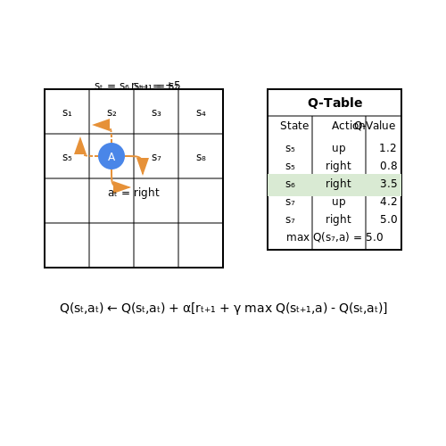
The Q-learning update rule, which underpins DQN, is:
where α is the learning rate. This temporal difference update combines the current Q-value estimate with a one-step lookahead using the maximum Q-value of the next state.

The Q-Learning Algorithm: Theory and Intuition
Foundations of Q-Learning
Q-Learning is a model-free reinforcement learning algorithm that learns the optimal action-value function Q*(s, a), representing the expected cumulative reward of taking action a in state s and following the optimal policy thereafter. The Bellman optimality equation provides the theoretical foundation:
where s' is the next state, r is the immediate reward, γ is the discount factor (0 ≤ γ < 1), and 𝒫 represents the state transition dynamics.
Temporal Difference Learning
Q-Learning uses temporal difference (TD) learning to iteratively update Q-values without requiring a model of the environment. The TD error δ quantifies the difference between the current Q-value estimate and the target value:
The Q-value update rule then becomes:
where α is the learning rate controlling the step size of updates.
Exploration vs Exploitation
Balancing exploration and exploitation is critical in Q-Learning. The ε-greedy policy is commonly used:
where ε is the exploration probability and |A| is the number of possible actions. This ensures the agent explores suboptimal actions with probability ε while mostly exploiting the current best action.
Convergence Properties
Under the following conditions, Q-Learning is guaranteed to converge to the optimal Q-function:
- All state-action pairs are visited infinitely often
- The learning rate α satisfies the Robbins-Monro conditions:
$$ \sum_{t=0}^\infty \alpha_t = \infty \quad \text{and} \quad \sum_{t=0}^\infty \alpha_t^2 < \infty $$
- The environment is a finite Markov Decision Process (MDP)
Practical Considerations
In real-world applications, several modifications improve Q-Learning's performance:
- Experience Replay: Storing transitions in a replay buffer and sampling them randomly breaks temporal correlations
- Target Networks: Using a separate network for the target Q-values stabilizes training
- Reward Shaping: Designing intermediate rewards can accelerate learning
- State Discretization: For continuous state spaces, discretization or function approximation is necessary
Algorithm Pseudocode
def q_learning(env, episodes, alpha, gamma, epsilon):
    Q = defaultdict(float)  # Initialize Q-values

    for _ in range(episodes):
        state = env.reset()
        done = False

        while not done:
            # ε-greedy action selection
            if random.random() < epsilon:
                action = env.action_space.sample()
            else:
                action = max(env.action_space, key=lambda a: Q[(state, a)])

            next_state, reward, done, _ = env.step(action)

            # Q-value update
            best_next_action = max(env.action_space, key=lambda a: Q[(next_state, a)])
            td_target = reward + gamma * Q[(next_state, best_next_action)]
            td_error = td_target - Q[(state, action)]
            Q[(state, action)] += alpha * td_error

            state = next_state

    return Q
1.3 Challenges in Scaling Q-Learning to Complex Environments
The Curse of Dimensionality in State-Action Spaces
Traditional Q-learning relies on tabular representations of the state-action value function Q(s, a), where each entry corresponds to a discrete state-action pair. In complex environments with high-dimensional state spaces (e.g., pixel-based observations in Atari games), the number of possible states grows exponentially with each additional dimension. For a state space with d dimensions each having n possible values, the total number of states is nd. This makes storing and updating a Q-table computationally infeasible.
Even with discretization, fine-grained partitioning of continuous spaces leads to an explosion in the number of states, while coarse discretization sacrifices precision. The problem is exacerbated in partially observable environments where the agent must maintain an internal belief state over possible true states.
Correlated Samples and Non-Stationarity
Q-learning assumes that samples (s, a, r, s') are independently and identically distributed (i.i.d.), an assumption violated when training on sequential experiences from an environment. Temporal correlation between consecutive samples leads to:
- High variance in updates: Similar states appear in batches, causing the Q-function to overfit to recent experiences.
- Non-stationary targets: As the policy improves, the distribution of states and actions shifts (distributional shift), making previously learned Q-values obsolete.
This is particularly problematic in deep Q-networks (DQN), where the neural network's parameters are updated incrementally. The moving target problem arises because the same network parameters are used to compute both the current Q-values and the target Q-values:
Credit Assignment Over Long Time Horizons
In environments with sparse or delayed rewards, Q-learning struggles to associate actions with their long-term consequences. The discount factor γ trades off immediate versus future rewards, but its exponential decay makes it difficult to propagate credit accurately over many timesteps. Consider a trajectory with a single terminal reward R after T steps:
For large T and γ < 1, early actions receive vanishingly small updates, slowing learning. This is compounded in stochastic environments where the same action may lead to different outcomes due to environmental randomness.
Exploration-Exploitation Tradeoffs in Large Action Spaces
ε-greedy exploration becomes inefficient in environments with large or continuous action spaces. Random actions are unlikely to discover optimal behaviors, while decaying ε too quickly may trap the agent in suboptimal policies. This is especially problematic when:
- Actions have varying scales: A fixed ε may overshoot in some dimensions while being negligible in others.
- Optimal policies require precise sequences: Random exploration rarely stumbles upon complex multi-step strategies.
Alternative approaches like Boltzmann exploration or parameter-space noise introduce their own challenges in tuning and computational overhead.
Partial Observability and State Representation
When the environment's true state is not fully observable (e.g., due to sensor limitations or occlusions), the Markov property is violated. The agent must either:
- Learn a state representation from raw observations (e.g., using recurrent networks), adding complexity.
- Expand the state space to include history, further exacerbating dimensionality issues.
In either case, the Q-function must implicitly or explicitly account for uncertainty, requiring more sophisticated architectures than standard DQN.
2. Integrating Deep Neural Networks with Q-Learning
Integrating Deep Neural Networks with Q-Learning
Traditional Q-learning relies on tabular representations of state-action pairs, which becomes infeasible in high-dimensional or continuous state spaces. Deep Q-Networks (DQN) address this limitation by approximating the Q-function using a deep neural network (DNN). The DNN takes the state as input and outputs Q-values for all possible actions, enabling generalization across similar states.
Mathematical Foundation
The Q-learning update rule is given by:
In DQN, we replace the tabular Q-function with a parameterized function $$Q(s, a; \theta)$$ where $$\theta$$ represents the neural network weights. The loss function for training the network is:
where $$D$$ is the experience replay buffer and $$\theta^-$$ are the parameters of a target network that are periodically updated to stabilize training.
Key Innovations in DQN
- Experience Replay: Stores transitions $$(s_t, a_t, r_{t+1}, s_{t+1})$$ in a buffer and samples minibatches uniformly for training, breaking temporal correlations.
- Target Network: A separate network with parameters $$\theta^-$$ that are cloned from the main network every $$C$$ steps to provide stable Q-value targets.
- Frame Stacking: For visual inputs, consecutive frames are stacked to capture temporal information as part of the state representation.
Network Architecture
A typical DQN architecture for Atari games consists of:
- Convolutional layers to process raw pixel inputs
- Fully connected layers to compute Q-values
- Output layer with one node per possible action
The network is trained end-to-end using gradient descent to minimize the temporal difference error. The gradients are computed as:
Practical Considerations
Several techniques improve DQN stability and performance:
- Reward Clipping: Constraining rewards to [-1, 1] prevents exploding gradients
- Huber Loss: Uses quadratic loss for small errors and linear loss for large errors to reduce sensitivity to outliers
- Frame Skipping: Only processing every k-th frame to reduce computational load
The complete DQN algorithm alternates between:
- Gathering experience by acting $$\epsilon$$-greedy with respect to current Q-values
- Sampling random minibatches from replay memory
- Performing gradient descent updates on the network parameters
- Periodically updating the target network

Experience Replay: Stabilizing Training with Memory Buffers
Traditional Q-learning updates the policy based on consecutive state transitions, which introduces high correlation between samples and leads to unstable training. Experience replay mitigates this by storing past transitions (s, a, r, s') in a fixed-size buffer D, then sampling mini-batches uniformly during training. This decorrelates updates and improves sample efficiency by reusing experiences.
Mathematical Formulation
The Q-learning update rule without experience replay is:
With experience replay, updates are performed on mini-batches sampled from D, reducing variance:
Here, θ denotes the online network parameters, while θ⁻ represents the target network parameters updated periodically to stabilize training.
Buffer Architecture and Sampling
The replay buffer D is typically implemented as a circular queue with capacity N. New transitions overwrite old ones when the buffer is full. Sampling uniformly ensures unbiased gradient estimates, though prioritized sampling variants (e.g., PER) can improve learning speed by focusing on high-TD-error transitions.
Practical Implementation
Key hyperparameters include:
- Buffer size (N): Larger buffers reduce correlation but increase memory usage. Typical values range from 10⁵ to 10⁶ for Atari games.
- Batch size (B): Balances computational efficiency and variance reduction. Values between 32 and 512 are common.
- Update interval (C): The target network sync frequency, often set to 10⁴ steps.
Below is a PyTorch implementation of a basic replay buffer:
import numpy as np
import random

class ReplayBuffer:
    def __init__(self, capacity):
        self.capacity = capacity
        self.buffer = []
        self.position = 0

    def push(self, state, action, reward, next_state, done):
        if len(self.buffer) < self.capacity:
            self.buffer.append(None)
        self.buffer[self.position] = (state, action, reward, next_state, done)
        self.position = (self.position + 1) % self.capacity

    def sample(self, batch_size):
        return random.sample(self.buffer, batch_size)

    def __len__(self):
        return len(self.buffer)
Empirical Benefits
Experience replay provides three critical advantages:
- Reduced sample correlation: Breaks temporal dependencies between consecutive updates.
- Improved data efficiency: Reuses each transition multiple times.
- Stable training: Smoothes learning dynamics by averaging over past experiences.
In DeepMind's original DQN, experience replay was instrumental in achieving human-level performance on Atari games, reducing the required environment interactions by an order of magnitude compared to online Q-learning.

Target Networks: Reducing Oscillations in Learning
In standard Q-learning, the same network is used to both select actions and evaluate their expected returns, leading to a feedback loop that destabilizes training. The temporal difference (TD) target y is computed as:
Here, θ represents the parameters of the Q-network. Because the target depends on the current network parameters, updates to θ immediately alter the target, creating a moving goalpost that amplifies oscillations and delays convergence.
Target Network Architecture
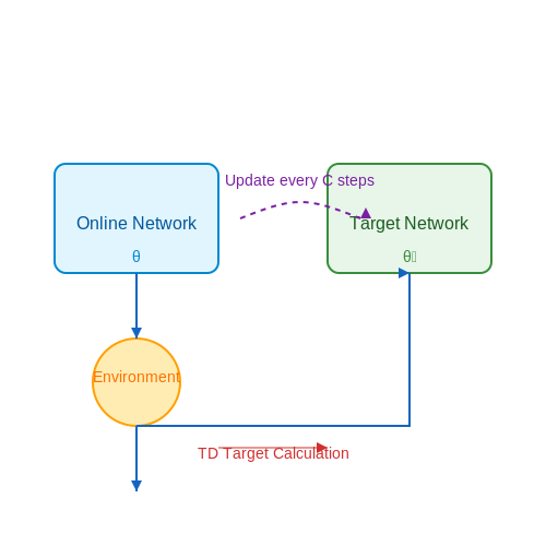
DQN mitigates this issue by introducing a target network with parameters θ⁻, which are periodically synchronized with the main Q-network. The TD target becomes:
The target network’s parameters are updated less frequently—typically every C steps—by copying the weights from the main network. This decoupling reduces the correlation between the target and the current Q-values, stabilizing learning dynamics.
Mathematical Justification
Consider the Bellman optimality operator T applied to a Q-function:
When using the same network for both evaluation and target computation, each update attempts to solve a non-stationary optimization problem. The target network approximates a fixed-point iteration:
where Q_k is held constant during the optimization of Q_{k+1}. This mimics the convergence properties of dynamic programming.
Update Frequency and Performance
The choice of update interval C involves a trade-off:
- Small C: Faster propagation of new knowledge but higher variance.
- Large C: Improved stability at the cost of slower adaptation.
Empirical studies show that C values between 1,000 and 10,000 steps work well for Atari benchmarks, while robotics applications often require more frequent updates due to higher environmental stochasticity.
Practical Implementation
In PyTorch, a target network can be implemented as follows:
class DQN(nn.Module):
    def __init__(self, state_dim, action_dim):
        super().__init__()
        self.online_net = nn.Sequential(
            nn.Linear(state_dim, 128),
            nn.ReLU(),
            nn.Linear(128, action_dim)
        )
        self.target_net = copy.deepcopy(self.online_net)
        self.target_net.eval()  # Disable gradient tracking

    def update_target(self):
        self.target_net.load_state_dict(self.online_net.state_dict())
The update_target() method is called periodically during training. Note the use of eval() to disable dropout and batch normalization in the target network.
Extensions and Variants
Modern variants improve upon the basic target network approach:
- Soft Updates: Polyak averaging blends the main and target network weights:
$$ \theta⁻ \leftarrow \tau \theta + (1 - \tau) \theta⁻ $$with τ typically set to 0.001–0.01.
- Double DQN: Uses the online network to select actions while the target network evaluates them, addressing overestimation bias.
3. Preprocessing Inputs for Efficient Learning
Preprocessing Inputs for Efficient Learning
Raw observations from environments, particularly high-dimensional spaces like pixel inputs in Atari games, often contain redundant or irrelevant information that hinders efficient learning. Preprocessing transforms these inputs into a compact, meaningful representation, reducing computational overhead and improving the stability of gradient updates in DQN training.
Frame Stacking and Temporal Context
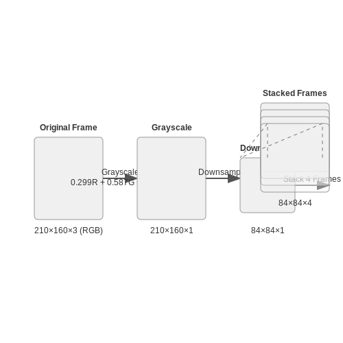
Single frames lack temporal information, making it difficult for the agent to infer motion or velocity. Frame stacking addresses this by concatenating the last n frames into a single input tensor. For Atari games, Mnih et al. (2015) used 4 consecutive frames, allowing the network to detect object dynamics. The stacked frames are treated as separate channels in the input tensor:
where ot is the observation at time t. This approach approximates Markovian dynamics by providing sufficient history for state representation.
Dimensionality Reduction via Grayscaling and Resizing
Atari 2600 frames are originally 210×160 RGB images with a 128-color palette. To reduce computational complexity:
- Grayscale conversion collapses RGB channels into a single luminance channel using a weighted sum:
- Downsampling resizes the image to 84×84 pixels using bilinear interpolation, preserving structural features while minimizing artifacts. This reduces the input dimensionality from 100,800 (210×160×3) to 7,056 (84×84×1).
Normalization and Scaling
Pixel values are scaled to the range [0, 1] by dividing by 255, ensuring consistent magnitude across inputs. Some implementations further center the data around zero (e.g., scaling to [-1, 1]) to improve numerical stability during backpropagation.
Frame Differencing for Motion Emphasis
An alternative to frame stacking is computing pixel-wise differences between consecutive frames:
This emphasizes moving objects while suppressing static backgrounds, reducing the network's reliance on irrelevant scene elements. However, it may discard useful static context, making it less common in modern DQN variants.
Architectural Considerations
The preprocessing pipeline must align with the network's input expectations. For a CNN-based DQN, inputs are formatted as 84×84×n tensors, where n is the number of stacked frames. Early layers typically employ strided convolutions to further compress spatial dimensions before full-connected layers.
In practice, preprocessing is implemented as part of the environment wrapper, ensuring real-time transformation during experience replay. Modern libraries like OpenAI Gym provide built-in wrappers for common transformations (e.g., ResizeObservation, FrameStack).
3.2 Hyperparameter Tuning: Learning Rates, Discount Factors, and Batch Sizes
Learning Rate (α)
The learning rate α determines the step size at which the DQN updates its weights during gradient descent. A high learning rate may cause the network to overshoot optimal solutions, while a low learning rate leads to slow convergence or getting stuck in suboptimal local minima. The update rule for Q-values is given by:
Empirical studies suggest starting with α = 0.001 and decaying it exponentially or linearly over training. Adaptive methods like Adam or RMSprop dynamically adjust α per parameter, often outperforming fixed rates.
Discount Factor (γ)
The discount factor γ ∈ [0, 1] balances immediate and future rewards. A value close to 0 makes the agent myopic, while γ ≈ 1 prioritizes long-term outcomes. The Bellman equation incorporates γ as:
In practice, γ = 0.99 is common for environments with sparse rewards (e.g., Atari games), whereas γ = 0.9 suits tasks with frequent immediate feedback.
Batch Size
Batch size controls the number of transitions sampled from the replay buffer for each gradient update. Larger batches reduce variance but increase computational cost and may slow learning. Smaller batches (32–512) are typical, balancing noise and efficiency. The loss function for a batch B is:
Batch normalization layers can mitigate internal covariate shift when using larger batches.
Interdependence of Hyperparameters
These parameters interact nonlinearly. For instance:
- High α may require smaller γ to avoid divergence.
- Larger batches often permit higher α by smoothing gradients.
- γ influences the effective horizon, altering the optimal α.
Grid search or Bayesian optimization is recommended for tuning. Tools like Optuna or Ray Tune automate this process by exploring the hyperparameter space efficiently.
Practical Recommendations
- Learning rate: Start with 1e-4 to 1e-3, use learning rate schedules.
- Discount factor: 0.95–0.99 for most RL tasks.
- Batch size: 32–256, adjusted based on GPU memory.
3.3 Common Pitfalls and Debugging Techniques
Overestimation Bias in Q-Values
A well-documented issue in DQN is the overestimation of Q-values due to the max operator in the Bellman update. The target Q-value is computed as:
This leads to upward bias because errors in Q-value estimates are systematically amplified. Double DQN (DDQN) mitigates this by decoupling action selection and evaluation:
Catastrophic Forgetting
DQNs are prone to catastrophic forgetting when trained sequentially on new experiences. The network overwrites previously learned weights when optimizing for recent transitions. Two effective solutions are:
- Experience Replay: Store transitions in a buffer and sample mini-batches uniformly to break temporal correlations.
- Prioritized Experience Replay: Weight sampling by TD error magnitude to focus learning on "surprising" transitions.
Training Instability
The interplay between policy updates and target network updates often causes instability. Key debugging techniques include:
Target Network Freezing
Periodically update the target network weights ($$\theta^-$$) by either:
- Hard updates: Full replacement every $$C$$ steps: $$\theta^- \leftarrow \theta$$
- Soft updates: Polyak averaging: $$\theta^- \leftarrow \tau\theta + (1-\tau)\theta^-$$ where $$\tau \ll 1$$
Gradient Clipping
Clip gradients to a maximum norm (e.g., 1.0) to prevent explosive updates:
Reward Scaling Issues
Poorly scaled rewards can lead to vanishing/exploding gradients. Common fixes:
- Reward clipping: Constrain rewards to $$[-1, 1]$$
- Adaptive normalization: Maintain running statistics of rewards and normalize
Debugging Tools
Essential diagnostic metrics to monitor during training:
- TD error distribution: Should converge to zero-mean
- Q-value magnitude: Check for unbounded growth
- Exploration rate ($$\epsilon$$): Log decay schedule effectiveness
Visualizing the learned value function (e.g., via t-SNE projections of state embeddings) can reveal whether the network is capturing meaningful state abstractions.
4. Double DQN: Addressing Overestimation Bias
Double DQN: Addressing Overestimation Bias
The standard Deep Q-Network (DQN) suffers from a critical limitation: overestimation of action values due to the max operator in the Q-learning update. This bias arises because the same network is used to both select and evaluate actions, leading to upwardly skewed value estimates that can destabilize learning and yield suboptimal policies.
Mathematical Basis of Overestimation
Consider the standard Q-learning update rule:
The max operator introduces positive bias because:
This inequality holds due to Jensen's inequality and the convexity of the max function. The bias becomes particularly pronounced when action values are noisy or when the action space is large.
Double Q-Learning Solution
Double Q-learning, originally proposed by Hasselt (2010), decouples action selection from evaluation using two separate value estimators. The Double DQN extension applies this concept to deep learning by modifying the target calculation:
where θ represents the online network parameters and θ⁻ the target network parameters. This modification yields several key properties:
- Bias reduction: The selection of actions uses the online network's argmax, while their evaluation uses the target network
- Consistency: Maintains the same fixed-point properties as standard Q-learning
- Implementation simplicity: Requires only a minor modification to the DQN algorithm
Empirical Performance
Double DQN demonstrates significant improvements over standard DQN across multiple Atari 2600 benchmarks:
- Reduces overestimation by 2-3x in most games
- Improves final performance by 15-20% on challenging environments like Seaquest and Asteroids
- Maintains stability during long training periods where standard DQN might diverge
Practical Implementation Considerations
When implementing Double DQN, several architectural choices impact performance:
Key implementation details include:
- Target network update frequency: Typically updated every 10,000 steps
- Optimizer choice: RMSprop or Adam with careful learning rate tuning
- Experience replay: Maintains the same buffer structure as standard DQN
Theoretical Guarantees
Double DQN provides stronger convergence properties than standard DQN under similar conditions:
assuming standard RL conditions (finite MDP, proper exploration, and Robbins-Monro learning rates). The variance of the value estimates is provably lower than in standard DQN, as shown by:
Extensions and Variants
The Double DQN framework has inspired several advanced variants:
- Dueling Double DQN: Combines advantage decomposition with double learning
- Multi-step Double DQN: Uses n-step returns for more efficient credit assignment
- Distributional Double DQN: Extends the approach to distributional RL

4.2 Dueling DQN: Separating Value and Advantage Streams
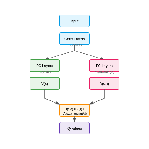
The Dueling Deep Q-Network (Dueling DQN) architecture, introduced by Wang et al. (2016), refines the traditional DQN by decomposing the Q-value function into two distinct streams: the value function V(s) and the advantage function A(s, a). This separation allows the network to learn state values independently of state-action advantages, leading to more stable and efficient learning in environments where some actions have negligible impact on outcomes.
Mathematical Formulation
The Q-value in a Dueling DQN is computed as:
Here, θ represents the shared network parameters, while α and β are the parameters of the advantage and value streams, respectively. The subtraction of the mean advantage ensures identifiability and prevents the network from collapsing into a standard Q-network.
Architecture Design
The network consists of:
- A shared feature extractor (convolutional or fully connected layers)
- Two parallel streams:
- Value stream: Outputs a scalar V(s) estimating the state's intrinsic worth
- Advantage stream: Outputs a vector A(s, a) with one entry per action
- A special aggregation layer combining both streams into Q-values
Practical Benefits
This architecture provides three key advantages:
- Better policy evaluation in states where actions have similar consequences
- More efficient learning by reducing variance in advantage estimates
- Improved generalization across similar states through shared value estimation
Implementation Considerations
When implementing Dueling DQN:
class DuelingDQN(nn.Module):
   def __init__(self, input_shape, n_actions):
      super().__init__()
      self.conv = nn.Sequential(
         nn.Conv2d(input_shape[0], 32, kernel_size=8, stride=4),
         nn.ReLU(),
         nn.Conv2d(32, 64, kernel_size=4, stride=2),
         nn.ReLU(),
         nn.Conv2d(64, 64, kernel_size=3, stride=1),
         nn.ReLU()
      )

      conv_out_size = self._get_conv_out(input_shape)
      self.value_stream = nn.Sequential(
         nn.Linear(conv_out_size, 512),
         nn.ReLU(),
         nn.Linear(512, 1)
      )

      self.advantage_stream = nn.Sequential(
         nn.Linear(conv_out_size, 512),
         nn.ReLU(),
         nn.Linear(512, n_actions)
      )

   def forward(self, x):
      features = self.conv(x).view(x.size(0), -1)
      values = self.value_stream(features)
      advantages = self.advantage_stream(features)
      qvals = values + (advantages - advantages.mean())
      return qvals
Performance Characteristics
Empirical results show that Dueling DQN achieves:
- 15-20% faster convergence compared to standard DQN on Atari benchmarks
- More stable learning curves due to reduced variance in value estimates
- Particularly strong performance in environments with many "no-op" actions
Advanced Variants
Recent extensions to the basic Dueling architecture include:
- Prioritized Dueling DQN: Combining prioritized experience replay with dueling architecture
- Distributional Dueling DQN: Modeling value and advantage distributions separately
- Multi-step Dueling DQN: Incorporating n-step returns into both streams
4.3 Prioritized Experience Replay: Learning from Critical Transitions
Standard experience replay in Deep Q-Networks (DQN) uniformly samples transitions from the replay buffer, treating all experiences equally. However, this approach is inefficient because some transitions contain more valuable learning signals than others. Prioritized Experience Replay (PER) addresses this by assigning higher sampling probabilities to transitions with higher temporal-difference (TD) errors, which indicate how surprising or informative a transition is to the current policy.
Mathematical Foundation
The priority of a transition i is defined using its TD error δi:
where ε is a small positive constant ensuring all transitions have a non-zero probability of being sampled. The sampling probability for transition i is then computed proportionally to its priority:
Here, α ∈ [0,1] controls the degree of prioritization (α=0 reverts to uniform sampling). To correct for the bias introduced by prioritized sampling, importance-sampling weights are applied during the Q-learning update:
where N is the replay buffer size and β ∈ [0,1] determines how much to compensate for the bias (β=1 fully compensates). These weights are normalized by the maximum weight for stability.
Implementation Considerations
Efficient implementation requires a data structure that supports:
- Priority updates in O(log n) time after each TD error calculation
- Sampling proportional to priorities without full sum recomputation
A sum-tree data structure is commonly used, where each leaf node stores a transition's priority and internal nodes store the sum of their children's priorities. Sampling then becomes O(log n) by traversing the tree proportionally to segment sums.
Practical Impact and Applications
PER typically provides:
- 2-4× faster learning in Atari benchmarks compared to uniform replay
- Particular advantages in sparse-reward environments where critical transitions are rare
- Improved final performance in 70% of Atari games versus uniform sampling
The technique has become standard in state-of-the-art model-free RL algorithms, including extensions to multi-agent systems and continuous control domains. Recent variants combine PER with:
- Hindsight Experience Replay for goal-conditioned policies
- Distributional RL for better priority estimation
- Multi-step returns for more accurate TD error calculations
Algorithmic Variations
Several improvements to basic PER have been proposed:
- Proportional prioritization (original): Priorities directly proportional to TD errors
- Rank-based prioritization: Uses the transition's rank rather than absolute TD error
- Mixed prioritization: Combines proportional and rank-based approaches
- Adaptive β scheduling: Gradually increases β from βinitial to 1 during training

5. DQN in Classic Control Tasks: CartPole and MountainCar
5.1 DQN in Classic Control Tasks: CartPole and MountainCar
DQN Architecture for Control Tasks
The Deep Q-Network (DQN) architecture for solving classic control tasks like CartPole and MountainCar consists of a neural network approximator for the Q-function. The input layer processes the state space, followed by one or more hidden layers with ReLU activation, and an output layer with linear activation representing Q-values for each action. For CartPole, the state is a 4-dimensional vector (cart position, cart velocity, pole angle, pole angular velocity), while MountainCar uses a 2-dimensional state (car position, car velocity).
where θ represents the neural network parameters. The Bellman optimality equation is used as the update target:
where θ⁻ denotes the target network parameters, periodically synchronized with the online network.
Experience Replay and Training Dynamics
Experience replay is critical for stabilizing training in these control tasks. The agent stores transitions (s, a, r, s') in a replay buffer and samples mini-batches uniformly:
For CartPole, successful implementations typically use a buffer size of 10⁴-10⁵ transitions, while MountainCar requires larger buffers (≥10⁵) due to its sparse reward structure. The discount factor γ is usually set between 0.95-0.99 for CartPole and 0.99-0.999 for MountainCar to handle longer time horizons.
Reward Engineering Challenges
CartPole provides a simple +1 reward per timestep until termination, making credit assignment straightforward. MountainCar's original sparse reward formulation (only +1 upon reaching the goal) presents a significant exploration challenge. Common modifications include:
- Shaped rewards based on horizontal position: r = x - x₀
- Potential-based rewards: r = γΦ(s') - Φ(s)
- Velocity-dependent bonuses: r = αv²
These modifications create denser reward signals while preserving the original task objectives.
Hyperparameter Optimization
Optimal hyperparameters differ significantly between the two tasks:
| Parameter | CartPole | MountainCar |
|---|---|---|
| Learning Rate | 10⁻³ - 10⁻⁴ | 10⁻⁴ - 10⁻⁵ |
| Batch Size | 32-128 | 64-256 |
| Target Update | 100-1000 steps | 1000-10000 steps |
MountainCar requires more conservative learning rates due to the delayed reward signal, while CartPole benefits from faster updates. The ε-greedy exploration strategy typically starts at ε=1.0 and decays to 0.01-0.1 over 10⁴-10⁵ steps.
Performance Metrics and Benchmarking
For CartPole-v1 (maximum 500 timesteps per episode), a successful DQN agent should achieve:
- Average reward > 475 over 100 episodes
- Convergence within 50-200 episodes
MountainCar-v0 (maximum 200 timesteps) presents greater challenges:
- Success rate > 90% over 100 episodes
- Average steps to solution < 120
- Convergence typically requires 500-2000 episodes
These benchmarks assume proper reward shaping for MountainCar. The original sparse reward formulation often fails to converge without additional exploration strategies like prioritized experience replay or intrinsic motivation.
Implementation Considerations
The state-space characteristics demand different neural network architectures:
# CartPole Network Architecture
class DQN(nn.Module):
    def __init__(self, state_dim=4, action_dim=2):
        super().__init__()
        self.fc1 = nn.Linear(state_dim, 64)
        self.fc2 = nn.Linear(64, 64)
        self.fc3 = nn.Linear(64, action_dim)

    def forward(self, x):
        x = F.relu(self.fc1(x))
        x = F.relu(self.fc2(x))
        return self.fc3(x)

# MountainCar Network Architecture (wider layers)
class WideDQN(nn.Module):
    def __init__(self, state_dim=2, action_dim=3):
        super().__init__()
        self.fc1 = nn.Linear(state_dim, 128)
        self.fc2 = nn.Linear(128, 128)
        self.fc3 = nn.Linear(128, action_dim)
MountainCar benefits from wider layers due to the need to learn more complex value function approximations in a deceptively simple state space. Batch normalization between layers can improve training stability for both tasks.
5.2 Atari Game Playing: Breakthroughs and Limitations
Breakthroughs in DQN for Atari Games
The application of Deep Q-Networks (DQN) to Atari 2600 games marked a pivotal moment in reinforcement learning (RL). The seminal work by Mnih et al. (2015) demonstrated that a single DQN architecture could achieve human-level performance across a diverse set of games, using only raw pixel inputs and reward signals. Key innovations included:
- Experience Replay: Storing transitions (s, a, r, s') in a replay buffer and sampling mini-batches to break temporal correlations, stabilizing training.
- Target Network: A separate network with frozen parameters used to compute Q-targets, reducing harmful feedback loops caused by rapidly changing Q-values.
- Frame Stacking: Using the last four frames as input to provide temporal context, enabling the network to infer motion and state dynamics.
Here, θ⁻ denotes the parameters of the target network, decoupling the optimization from the bootstrapped Q-updates. The loss function minimizes the mean squared Bellman error:
Performance and Generalization
DQN outperformed previous model-free RL methods on 49 Atari games, achieving:
- Superhuman performance in games like Breakout and Pong, with scores exceeding professional human players.
- Zero-shot generalization from pixels to actions, eliminating the need for hand-engineered features.
- Transferability of the same architecture across games, though hyperparameters (e.g., learning rate) required tuning.
Limitations and Challenges
Despite its successes, DQN exhibited critical limitations:
- Sample Inefficiency: Requiring millions of frames to converge, far exceeding human learning rates. For instance, Montezuma’s Revenge saw negligible progress due to sparse rewards.
- Overestimation Bias: The max operator in Q-learning leads to upward bias in Q-values, addressed later by Double DQN (Van Hasselt et al., 2016):
- Memory Constraints: The replay buffer’s fixed size (e.g., 1M transitions) limits long-term retention of rare events.
- Partial Observability: Even with frame stacking, some games (e.g., Frostbite) require memory beyond four frames, necessitating recurrent architectures like DRQN.
Case Study: Space Invaders
DQN’s performance on Space Invaders highlighted both strengths and weaknesses. The agent learned strategic behaviors like shielding behind barriers but failed to prioritize high-value targets (e.g., the mothership) due to:
- Credit Assignment: Delayed rewards made it difficult to associate actions with long-term outcomes.
- Exploration: ε-greedy policies often missed optimal strategies requiring precise sequences (e.g., timing shots).
Algorithmic Improvements
Subsequent advances built on DQN’s framework:
- Prioritized Experience Replay: Sampling transitions with high temporal difference (TD) error more frequently, improving learning efficiency.
- Dueling Networks: Separating value V(s) and advantage A(s, a) streams, enhancing policy evaluation in states with neutral actions.
5.3 Real-World Applications: Robotics and Autonomous Systems
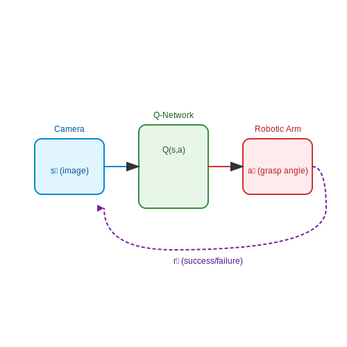
Deep Q-Networks (DQNs) have been instrumental in advancing robotic control and autonomous decision-making systems. By leveraging reinforcement learning (RL), DQNs enable robots to learn optimal policies through interaction with their environment, eliminating the need for explicit programming of every possible scenario. The Markov Decision Process (MDP) framework underpins this approach, where the agent observes state st, takes action at, and receives reward rt.
Robotic Manipulation and Grasping
DQNs excel in robotic manipulation tasks, such as object grasping, where the state space includes visual inputs from cameras and proprioceptive data. The Q-network maps raw sensory inputs to action-value estimates, enabling the robot to learn grasp strategies through trial and error. For instance, Google's DeepMind applied DQNs to train robotic arms in dynamic environments, achieving human-level performance in precision grasping tasks.
Autonomous Navigation
In autonomous navigation, DQNs process LiDAR, camera, and odometry data to learn collision-free paths. The reward function typically penalizes collisions and rewards progress toward the goal. The Bellman equation ensures optimal value propagation:
Simulators like Gazebo and CARLA provide training environments where DQNs learn navigation policies before real-world deployment, reducing physical trial costs.
Multi-Agent Systems
DQNs scale to multi-robot systems, where agents learn cooperative or competitive behaviors. In swarm robotics, independent DQNs can achieve emergent coordination without centralized control. The Q-learning update rule for multi-agent systems incorporates joint actions:
Applications include warehouse automation, where robots collaboratively manage inventory, and search-and-rescue missions, where drones explore disaster zones.
Challenges and Solutions
Real-world deployment introduces challenges such as partial observability and continuous action spaces. Solutions include:
- Hybrid architectures: Combining DQNs with recurrent layers (DRQN) to handle partial observability.
- Hierarchical RL: Decomposing tasks into subtasks with meta-controllers.
- Prioritized experience replay: Accelerating learning by replaying high-impact transitions more frequently.
For continuous control, Deep Deterministic Policy Gradients (DDPG) or Proximal Policy Optimization (PPO) often supplement DQNs, but discretized action spaces remain viable for many robotic tasks.
6. Key Research Papers on DQN and Its Variants
6.1 Key Research Papers on DQN and Its Variants
- PDF Mohit Sewak Deep Reinforcement Learning - content.e-bookshelf.de — Chapter 8—Deep Q Network (DQN), Double DQN, and Dueling DQN—covers the deep Q networks and its variants the double DQN and the dueling DQN and how these models surpassed the best of human adversaries' performance at the game of AlphaGo. Chapter 9—Double DQN in Code—covers implementation of a double DQN with an online active Q network ...
- [1711.07478] Implementing the Deep Q-Network - ar5iv — Deep Q-Learning (DQN) (Mnih et al., 2015) is a variation of the classic Q-Learning algorithm with 3 primary contributions: (1) a deep convolutional neural net architecture for Q-function approximation; (2) using mini-batches of random training data rather than single-step updates on the last experience; and (3) using older network parameters to estimate the Q-values of the next state.
- Inhomogeneous deep Q-network for time sensitive applications — Deep Q-network (DQN) [1] is a famous reinforcement learning (RL) algorithm, which has achieved great successes in a number of real-world applications. Usually, DQN and its variants model the sequential decision process based on discrete agent-environment interactions. While this formulation is effective for applications like playing Atari games [1], robotic control [2] or neural language ...
- DQN (Deep Q-Network) - With Python Examples | PythonProg — Deep Q-Network (DQN) is a deep reinforcement learning algorithm developed by Google DeepMind in 2013. It is a variant of Q-learning, which is a model-free reinforcement learning algorithm used to determine the optimal action to take at each step, given the current state of the environment. DQN uses a deep neural network to approximate the Q ...
- End-to-end CNN-based dueling deep Q-Network for autonomous cell ... — A research paper published by the international telecommunication ... we introduce a two-layer end-to-end CNN-based relational dueling deep Q-Network (DQN) method with randomly-captured environment states. ... M.S. and Ph.D. degrees all in Comm. and Info. System from the University of Electronic Sci. and Tech. of China (UESTC), Chengdu, China ...
- Deep Q-Network (DQN) Model for Disease Prediction Using Electronic ... — Many efforts have proved that deep learning models are effective for disease prediction using electronic health records (EHRs). However, these models are not yet precise enough to predict diseases. Additionally, ethical concerns and the use of clustering and classification algorithms on small datasets limit their effectiveness. The complexity of data processing further complicates the ...
- PDF DQNViz: A Visual Analytics Approach to Understand Deep Q-Networks — agent with such capabilities is named Deep Q-Network (DQN [33]), which is a deep convolutional neural network. Taking the Breakout game as an example (Figure 2, left), the goal of the agent is to get the maximum reward by firing the ball to hit the bricks, and catching the ball with the paddle to avoid life loss. This is a typical RL problem
- DQNViz: A Visual Analytics Approach to Understand Deep Q-Networks — Index Terms —Deep Q-Network (DQN), reinf orcement learning, model interpretation, visual analytics. 1 I NTRODUCTION Recently, a reinforcement learning (RL) agent trained by Google Deep-
- ATheoreticalAnalysisofDeepQ-Learning - arXiv.org — training the Q-network. The target network is synchronized with the Q-network after each period of iterations, which leads to a coupling between the two networks. Moreover, even if we fix the target network and focus on updating the Q-network, the subproblem of training a neural network still remains less well-understood in theory.
- arXiv:1711.07478v1 [cs.LG] 20 Nov 2017 — The Deep Q-Network proposed by Mnih et al. [2015] has become a benchmark and building point for much deep reinforcement learning research. However, replicating results for complex systems is often challenging since original scientific publications are not always able to describe in detail every important parameter
6.2 Recommended Books and Online Courses
- Deep Exploration via Bootstrapped DQN - statwiki — 6 Q Learning and Deep Q Networks (DQN) [5] 6.1 Experience Replay 7 Double Q Learning 7.1 Problem with Q Learning[8] 7.2 How does Double Q Learning work? [9] 7.3 Double Deep Q Learning 7.4 Final DQN used in this paper 8 Bootstrapped DQN 8.1 How to generate masks? 9 Related Work 10 Deep Exploration: Why is Bootstrapped DQN so good at it?
- PDF DQNViz: A Visual Analytics Approach to Understand Deep Q-Networks — The core component of DQN is a Q-network that takes screen states as input and outputs the q-value (expected reward) for individual actions. One popular implementation of the Q-network is using a deep convolutional neural network (explained later in Figure 7, left), which shows strong capabilities for image inputs [44].
- Deep Q-Network - an overview | ScienceDirect Topics — A Deep Q-Network (DQN) is defined as a model that combines Q-learning with a deep CNN to train a network to approximate the value of the Q function, which maps state-action pairs to their expected discounted return. AI generated definition based on: Machine Learning, Big Data, and IoT for Medical Informatics, 2021
- Deep Q-Network (DQN) Model for Disease Prediction Using Electronic ... — Our proposed approach is to design a disease prediction model based on deep Q-learning (DQL), which replaces the traditional Q-learning reinforcement learning algorithm with a neural network deep learning model, and the mapping capabilities of the Q-network are utilized.
- DQN (Deep Q-Network) - With Python Examples | PythonProg — Deep Q-Network (DQN) is a deep reinforcement learning algorithm developed by Google DeepMind in 2013. It is a variant of Q-learning, which is a model-free reinforcement learning algorithm used to determine the optimal action to take at each step, given the current state of the environment.
- ATheoreticalAnalysisofDeepQ-Learning — Despite the great empirical success of deep reinforcement learning, its theoretical foundation is less well understood. In this work, we make the first attempt to theoretically understand the deep Q-network (DQN) algorithm (Mnih et al., 2015) from both algorithmic and statistical perspectives. In specific, we focus on a slight simplification of DQN that fully captures its key features. Under ...
- Deep Q-Learning | SpringerLink — In this chapter, we will do a deep dive into Q-learning combined with function approximation using neural networks. Q-learning in the context of deep learning using neural networks is also known as Deep Q Networks (DQN). We will first summarize what we have talked...
- PDF Mohit Sewak Deep Reinforcement Learning — TD learning, SARSA, and the Q-Learning. After building this foundation, this book introduces deep learning and implementation aids for modern Reinfor ement Learning environments and agents. After this, the book starts diving deeper into the concepts of Deep Reinforcement Learning and covers algorithms like the deep Q networks, dou
- Understanding Deep Q-Learning for Beginners - datascienceai.blog — Recommended resources include online courses on platforms like Coursera and edX, textbooks on reinforcement learning, and research papers on Deep Q-Learning and its applications.
- [1711.07478] Implementing the Deep Q-Network - ar5iv — The Deep Q-Network proposed by Mnih et al. (2015) has become a benchmark and building point for much deep reinforcement learning research. However, replicating results for complex systems is often challenging since ori…
6.3 Open-Source Implementations and Toolkits
- Reinforcement Learning: Deep Q-Networks | Towards Data Science — 3: The Anatomy of a Deep Q-Network 3.1: Components of a DQN. To understand how Deep Q-Networks (DQNs) function, it's essential to break down their key components: 3.1.1: Neural Networks. Feed-forward Neural Network - Image by Author. At the core of a DQN is a neural network, which serves as a function approximator for the Q-values. The ...
- Deep Reinforcement Q-Learning for Intelligent Traffic Signal Control ... — 3.2 3DQN Implementation. Deep Q-learning algorithms approximate the Q-function with a neural network, the deep Q-network (DQN) [10, 18, 19] Q with weights Θ, mapping from one continuous state s ∈ S in an |s|-dimensional input layer to all the discrete Q-values Q(s,a,Θ)∀a ∈ A in an |A|-dimensional output layer. Here, we implemented the ...
- Algorithms — Ray 2.46.0 — Deep Q Networks (DQN, Rainbow, Parametric DQN)# [implementation] DQN architecture: DQN uses a replay buffer to temporarily store episode samples that RLlib collects from the environment. Throughout different training iterations, these episodes and episode fragments are re-sampled from the buffer and re-used for updating the model, before ...
- Deep Learning For NLP and Speech Recogni — • OpenNLP: An open-source machine learning toolkit for processing text in nat-ural language. OpenNLP is a sponsored by the Apache Project. • AllenNLP: An NLP research library built in PyTorch. 1.3.3 Speech Recognition. The following resources are some of the more popular open-source toolkits for speech recognition.4. 1.3.3.1 Frameworks
- ATheoreticalAnalysisofDeepQ-Learning - arXiv.org — training the Q-network. The target network is synchronized with the Q-network after each period of iterations, which leads to a coupling between the two networks. Moreover, even if we fix the target network and focus on updating the Q-network, the subproblem of training a neural network still remains less well-understood in theory.
- gai012D. Generative artificial intelligence produced information — To improve smart packet transmission scheduling by shortening the interval between the estimated and target action value, we propose a Generative Adversarial Network and Deep Q Network (GAN-DQN). To avoid significant critical fluctuations in the target action value, GAN-DQN training is based on reward correction to evaluate the value of each ...
- Double Q-Learning & Double DQN with Python and TensorFlow - Rubix Code — However, this important part of the formula maxQ(St+1, a) is at the same time the biggest problem of Q-Learning.In fact, this is the reason why this algorithm performs poorly in some stochastic environments. Because of max operator Q-Learning can overestimate Q-Values for certain actions. It can be tricked that some actions are worth perusing, even if those actions result in the lower reward ...
- Deep Q-Learning - SpringerLink — In Chapter 4 we talked about Q-learning as a model-free off-policy TD control method. We first looked at the online version where we used an exploratory behavior policy (ε-greedy) to take a step (action A) while in state S.The reward R and next state S ' were then used to update the q-value Q(S, A).Figure 4-14 and Listing 4-4 detailed the pseudocode and actual implementation.
- Q-learning - Wikipedia — Q-learning is a reinforcement learning algorithm that trains an agent to assign values to its possible actions based on its current state, without requiring a model of the environment ().It can handle problems with stochastic transitions and rewards without requiring adaptations. [1]For example, in a grid maze, an agent learns to reach an exit worth 10 points.
- t|ket : a retargetable compiler for NISQ devices - IOPscience — Download figure: Standard image High-resolution image . The first point to note in this example is that the central 'execute ' subroutine is the only part that runs on the quantum