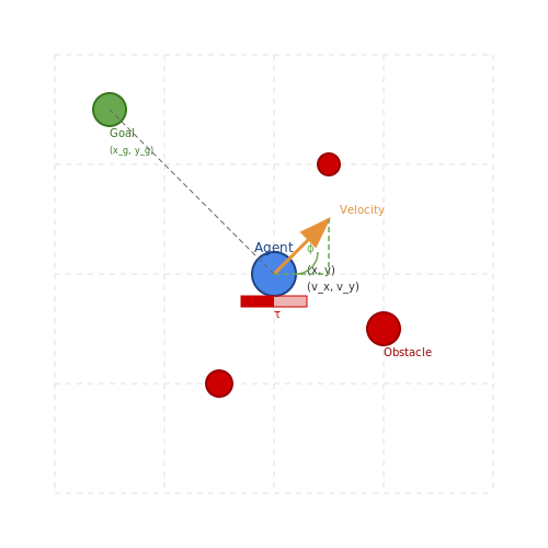
Exploration vs Exploitation Strategies
1. Definition and Core Trade-off
Exploration vs Exploitation: Definition and Core Trade-off
The exploration-exploitation dilemma arises in sequential decision-making problems where an agent must balance between gathering new information (exploration) and leveraging existing knowledge to maximize rewards (exploitation). This trade-off is fundamental to reinforcement learning, multi-armed bandits, and optimal control.
Mathematical Formulation
Consider a multi-armed bandit problem with K arms, where each arm i yields rewards drawn from an unknown distribution with mean μi. At each time step t, the agent selects an arm at and observes a reward rt. The cumulative regret after T steps is:
where μ* = maxi μi is the optimal mean reward. The goal is to minimize regret by carefully balancing exploration and exploitation.
The Core Trade-off
The tension between exploration and exploitation manifests in several ways:
- Information Gain vs Immediate Reward: Exploring suboptimal arms provides information about their reward distributions, while exploiting the current best arm maximizes immediate rewards.
- Short-term vs Long-term Performance: Excessive exploitation may lead to suboptimal long-term performance if better options remain undiscovered.
- Uncertainty Reduction: Exploration reduces uncertainty about arm rewards, enabling more informed future decisions.
Regret Bounds and Fundamental Limits
Lai and Robbins (1985) established that any consistent policy must satisfy the asymptotic lower bound on regret:
where KL denotes the Kullback-Leibler divergence between the reward distributions of arm i and the optimal arm. This result highlights the fundamental difficulty of the exploration-exploitation trade-off.
Practical Considerations
In real-world applications, the trade-off is further complicated by:
- Non-stationarity: Reward distributions may change over time, requiring continuous exploration.
- Partial Observability: The agent may only observe rewards for selected actions, not all possibilities.
- High-dimensional Action Spaces: The number of possible actions may be extremely large, making exhaustive exploration infeasible.
Visualizing the Trade-off
The exploration-exploitation trade-off can be visualized as a Pareto frontier where increased exploration leads to higher information gain but lower immediate rewards, while increased exploitation yields higher short-term rewards but potentially suboptimal long-term performance. The optimal strategy depends on the time horizon and the agent's uncertainty about the environment.

Key Applications in Reinforcement Learning
The exploration-exploitation trade-off is fundamental to reinforcement learning (RL), where an agent must balance gathering new information (exploration) with leveraging known information to maximize rewards (exploitation). Advanced RL applications often require sophisticated strategies to handle this trade-off effectively.
Multi-Armed Bandit Problems
The multi-armed bandit (MAB) framework is the simplest setting where exploration-exploitation strategies are critical. Here, an agent repeatedly chooses among k actions (arms), each providing a stochastic reward. The goal is to maximize cumulative reward over time. Upper Confidence Bound (UCB) and Thompson Sampling are two widely-used algorithms:
where Qt(a) is the estimated value of action a, Nt(a) is the number of times action a has been selected, and c is a hyperparameter controlling exploration.
Markov Decision Processes (MDPs)
In MDPs, exploration-exploitation strategies extend to sequential decision-making. Algorithms like Q-Learning and SARSA balance exploration (e.g., ε-greedy, softmax) with exploitation:
Here, ε-greedy policies select the greedy action with probability 1-ε and a random action otherwise, ensuring continual exploration.
Deep Reinforcement Learning
In deep RL, exploration strategies must scale to high-dimensional state spaces. Techniques like:
- Noisy Networks: Add parametric noise to weights, enabling stochasticity without explicit sampling.
- Intrinsic Motivation: Use curiosity-driven rewards (e.g., prediction error) to encourage exploration.
- Bootstrapped DQN: Ensemble of Q-networks with randomized initializations to guide exploration.
Real-World Applications
Practical implementations include:
- Autonomous Systems: Robotics navigation where agents must explore unknown environments while optimizing paths.
- Recommendation Engines: Balancing exploitation of known user preferences with exploration of new items.
- Healthcare: Clinical trials where treatments (arms) must be explored while maximizing patient outcomes.
Non-Stationary Environments
In dynamic settings, reward distributions change over time, requiring adaptive strategies. Algorithms like Sliding-Window UCB or Discounted Thompson Sampling discount older observations to focus on recent data:
where θa(t) is the sampled reward mean for action a, and Na(t) is the discounted count of selections.
1.3 Real-world Analogies and Intuition
The exploration-exploitation tradeoff manifests in everyday decision-making, often subconsciously. Consider a restaurant selection problem: a diner must choose between a familiar favorite (exploitation) and a new, potentially better option (exploration). The optimal strategy balances known rewards with the uncertainty of untried alternatives. This mirrors multi-armed bandit problems, where the regret of not discovering high-reward actions must be minimized.
Investment Portfolios
In finance, investors allocate capital between stable assets (exploitation) and high-risk ventures (exploration). The Kelly criterion provides a mathematical framework for this balance:
where f* is the fraction of capital to risk, b the net odds, p the win probability, and q = 1 - p. Over-betting leads to ruin (over-exploitation), while under-betting misses growth (over-exploration).
Clinical Trials
Adaptive trials allocate patients to treatments dynamically. The Thompson sampling method models this as a Bayesian optimization:
where π(a) is the probability of selecting action a given observed data 𝒟. This balances exploring under-tested drugs against exploiting known efficacies.
Evolutionary Strategies
Biological systems exhibit exploration through mutation rates. The 1/5 success rule in evolution strategies adapts the mutation strength σ:
where ps is the success rate and c ≈ 0.817 a tuning constant. This maintains diversity (exploration) while converging to fit traits (exploitation).
Hyperparameter Optimization
Neural architecture search uses exploration-exploitation in weight space. The Upper Confidence Bound (UCB) acquisition function formalizes this:
where μ is the mean reward (exploitation), σ the uncertainty (exploration), and κ a tradeoff parameter. This parallels A/B testing in web design, where UCB variants optimize click-through rates.
2. Epsilon-Greedy Method
2.1 Epsilon-Greedy Method
The epsilon-greedy strategy is a fundamental approach to balancing exploration and exploitation in reinforcement learning. At each decision step, the agent selects the action with the highest estimated value (exploitation) with probability 1 - ε, while choosing a random action (exploration) with probability ε. This ensures a controlled trade-off between refining current knowledge and discovering potentially better actions.
Mathematical Formulation
The action selection policy in epsilon-greedy is defined as:
Here, Qt(a) represents the estimated value of action a at time t. The parameter ε ∈ [0,1] controls the exploration rate. A value of ε = 0 reduces the policy to pure greediness, while ε = 1 results in purely random exploration.
Convergence Properties
Under stationary reward distributions, the epsilon-greedy method guarantees asymptotic convergence to the optimal policy if ε is annealed over time according to:
where c and d are problem-dependent constants, and t is the timestep. This decay schedule ensures sufficient exploration early on while gradually shifting toward exploitation as value estimates become more accurate.
Practical Implementation Considerations
In non-stationary environments where reward distributions change over time, a fixed ε is often preferred to maintain continual exploration. Common values range from 0.01 to 0.1 in production systems. The method's computational efficiency—requiring only O(1) operations per action selection—makes it widely applicable in large-scale systems.
Variants and Enhancements
- Decaying Epsilon-Greedy: Reduces exploration over time, often using exponential decay: εt = ε0αt
- Adaptive Epsilon: Dynamically adjusts ε based on uncertainty measures or performance metrics
- Optimistic Initialization: Combines with high initial Q-values to encourage systematic early exploration
Performance Analysis
The regret bound for standard epsilon-greedy in a k-armed bandit problem is linear in the worst case, but improved variants achieve O(log T) regret. The exact bound depends on the gap Δ between optimal and suboptimal actions:
where a* denotes the optimal action. This highlights the direct trade-off between exploration cost (first term) and exploitation benefit (second term).
Upper Confidence Bound (UCB)
The Upper Confidence Bound (UCB) algorithm is a principled approach to balancing exploration and exploitation in multi-armed bandit problems. Unlike ε-greedy methods, which explore randomly, UCB quantifies the uncertainty of reward estimates and systematically favors actions with high potential.
Mathematical Foundation
UCB constructs a confidence interval around the estimated mean reward for each action and selects the action with the highest upper bound. The UCB1 variant, one of the most widely used formulations, is derived from the Chernoff-Hoeffding bound:
where:
- \(\hat{\mu}_i\) is the empirical mean reward of action \(i\)
- \(t\) is the total number of rounds played
- \(n_i\) is the number of times action \(i\) has been selected
Derivation of the Confidence Term
The confidence term \(\sqrt{2 \ln t / n_i}\) emerges from analyzing the tail bounds of sub-Gaussian distributions. For a reward distribution with support in [0,1], the Hoeffding inequality gives:
Setting the right-hand side equal to \(t^{-4}\) (to ensure summable probabilities over time) and solving for ε yields the UCB1 exploration term. This guarantees that the true mean lies within the confidence interval with high probability.
Regret Analysis
UCB1 achieves logarithmic regret, which is asymptotically optimal. The cumulative regret after \(T\) rounds is bounded by:
where \(\Delta_i = \mu^* - \mu_i\) is the suboptimality gap of action \(i\). This bound shows that UCB pays only logarithmic penalty for suboptimal actions while maintaining constant terms for the best arm.
Practical Variants
Several improved variants address limitations of UCB1:
- KL-UCB: Uses Kullback-Leibler divergence for tighter bounds on Bernoulli rewards
- UCB-Tuned: Incorporates empirical variance estimates for better performance
- Bayesian UCB: Uses posterior distributions instead of frequentist confidence intervals
For Gaussian rewards with unknown mean and variance, the UCB-Normal algorithm modifies the confidence term to:
where \(\sigma_i^2\) is the empirical variance of rewards from action \(i\).
Implementation Considerations
Key practical aspects when implementing UCB include:
- Initialization strategies for cold-start problems
- Handling non-stationary environments through sliding windows or discount factors
- Parallelization in distributed systems
- Computation of confidence bounds for high-dimensional action spaces
In contextual bandits, UCB principles extend to linear models through the LinUCB algorithm, which maintains confidence ellipsoids around parameter estimates.

2.3 Thompson Sampling
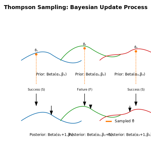
Thompson Sampling, also known as posterior sampling, is a Bayesian heuristic for balancing exploration and exploitation in stochastic multi-armed bandit problems. Unlike deterministic methods like UCB, Thompson Sampling maintains a probability distribution over the expected rewards of each arm and samples from these distributions to select actions. This approach naturally balances exploration and exploitation by leveraging uncertainty in the estimated reward distributions.
Bayesian Framework
Thompson Sampling operates within a Bayesian framework, where each arm's reward distribution is modeled with a prior that is updated as observations are made. For Bernoulli bandits, a common choice is the Beta distribution as a conjugate prior for the Bernoulli likelihood. The algorithm proceeds as follows:
- Initialize priors for each arm (e.g., Beta(1,1) for a uniform prior).
- For each round:
- Sample a reward probability from the current posterior of each arm.
- Select the arm with the highest sampled value.
- Observe the reward and update the posterior distribution of the selected arm.
where \(\theta_a\) is the reward probability of arm \(a\), \(D\) is the observed data, \(P(\theta_a)\) is the prior, and \(P(D | \theta_a)\) is the likelihood.
Algorithm Derivation
For a Bernoulli bandit with a Beta(α, β) prior, the posterior after observing \(S\) successes and \(F\) failures is Beta(α + S, β + F). The Thompson Sampling algorithm samples from these posteriors:
The arm with the highest \(\tilde{\theta}_a\) is selected. This sampling step inherently balances exploration (selecting arms with uncertain but potentially high rewards) and exploitation (selecting arms known to yield high rewards).
Regret Analysis
Thompson Sampling achieves near-optimal regret bounds. For a K-armed bandit with Bernoulli rewards, the expected cumulative regret after \(T\) rounds is bounded by:
This matches the lower bound for stochastic bandits up to logarithmic factors, demonstrating its efficiency.
Extensions and Variants
Thompson Sampling generalizes beyond Bernoulli bandits:
- Gaussian Bandits: Use Normal-Gaussian conjugate priors for normally distributed rewards.
- Contextual Bandits: Incorporate linear models or neural networks to handle contextual information.
- Nonparametric Bandits: Employ Dirichlet processes or Gaussian processes for flexible reward modeling.
Practical Considerations
Thompson Sampling is computationally efficient, especially with conjugate priors, as posterior updates are closed-form. However, for complex models (e.g., deep neural networks), approximate inference techniques like variational inference or MCMC may be required. The algorithm's probabilistic nature also makes it robust to delayed feedback and non-stationary environments.
Applications
Thompson Sampling is widely used in:
- Online Advertising: Optimizing ad displays based on click-through rates.
- Clinical Trials: Adaptively assigning treatments to maximize patient outcomes.
- Recommendation Systems: Personalizing content while exploring user preferences.
2.4 Optimism in the Face of Uncertainty
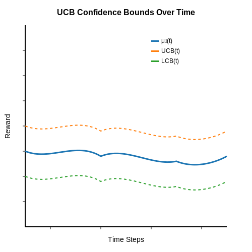
Optimism in the Face of Uncertainty (OFU) is a mathematically grounded exploration strategy that systematically biases action selection toward under-sampled regions with high potential reward. The core principle is to construct an upper confidence bound (UCB) on the expected reward of each action, then greedily select the action with the highest bound. This approach ensures provable regret bounds while maintaining efficient exploration.
Mathematical Formulation
Given a multi-armed bandit problem with K arms, let μi be the true mean reward of arm i and ni(t) its pull count by time t. The UCB1 algorithm selects arms according to:
where μ̂i(t) is the empirical mean reward. The second term represents the exploration bonus, which decays with pull count but grows logarithmically over time.
Generalized Linear Bandits
For contextual bandits with feature vector xt,a and unknown parameter θ*, LinUCB constructs confidence ellipsoids:
where At = λI + Σxs,axs,aT is the design matrix and βt is a confidence radius derived from concentration inequalities. The action selection rule becomes:
Practical Considerations
- Tight confidence bounds: The Hoeffding-based UCB1 bound is often loose; alternatives like KL-UCB use divergence-based bounds for better finite-time performance.
- Non-stationarity: Discounted or sliding-window UCB variants maintain optimism in changing environments.
- High-dimensional spaces: Sparse OFU methods like Lasso-UCB exploit sparsity through regularization.
Theoretical Guarantees
For a K-armed bandit with subgaussian rewards, UCB1 achieves regret:
where Δi = μ* - μi is the suboptimality gap. This logarithmic regret bound is asymptotically optimal for stationary environments.
3. Bayesian Exploration Methods
3.1 Bayesian Exploration Methods
Bayesian exploration methods provide a principled framework for balancing exploration and exploitation by maintaining a probability distribution over possible reward models. These methods leverage Bayesian inference to update beliefs about the environment dynamically, allowing for optimal decision-making under uncertainty.
Bayesian Bandits
In the context of multi-armed bandits, Bayesian methods model the reward distribution of each arm using a prior distribution, which is updated as observations are made. The posterior distribution reflects the updated belief about the expected reward, guiding the exploration-exploitation trade-off.
Here, θ represents the parameters of the reward distribution, D is the observed data, P(θ) is the prior, P(D | θ) is the likelihood, and P(θ | D) is the posterior.
Thompson Sampling
Thompson Sampling is a widely used Bayesian exploration strategy that samples from the posterior distribution to select actions probabilistically. For each decision, a candidate reward parameter is drawn from the posterior, and the action with the highest sampled reward is chosen.
This approach naturally balances exploration and exploitation, as actions with uncertain but potentially high rewards are occasionally selected.
Gaussian Process Bandits
For continuous action spaces, Gaussian Process (GP) bandits extend Bayesian methods by modeling the reward function as a GP. The GP provides a distribution over possible functions, enabling uncertainty quantification and optimal exploration.
Here, m(x) is the mean function, and k(x, x') is the kernel function defining covariance. Acquisition functions like Expected Improvement (EI) or Upper Confidence Bound (UCB) guide exploration:
where μ(x) is the predicted mean, σ(x) is the standard deviation, and β controls exploration.
Practical Applications
Bayesian exploration methods are widely used in:
- Hyperparameter Optimization: Efficiently navigating high-dimensional parameter spaces in machine learning.
- Clinical Trials: Adaptively allocating treatments to maximize patient outcomes while minimizing risk.
- Recommendation Systems: Balancing exploration of new items with exploitation of known preferences.
Intrinsic Motivation and Curiosity-Driven Learning
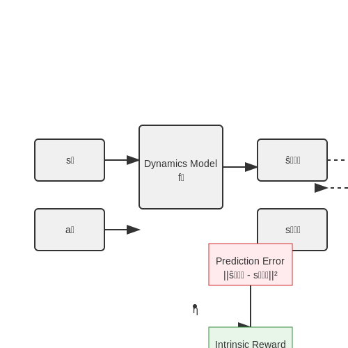
Intrinsic motivation in reinforcement learning refers to an agent's drive to explore its environment based on internal rewards rather than external incentives. Unlike traditional reward-driven exploration, intrinsic motivation mechanisms encourage agents to seek novel or informative states, leading to more robust learning in sparse-reward environments. One formalization of this concept is through information gain, where the agent maximizes the reduction in uncertainty about its environment model.
Mathematical Formulation of Curiosity
The curiosity-driven reward rtintrinsic at time t can be modeled as the prediction error of a learned dynamics model fϕ:
where η is a scaling factor, ŝt+1 = fϕ(st, at) is the predicted next state, and st+1 is the observed next state. This prediction error serves as a proxy for how "surprising" a state transition is to the agent.
Variational Information Maximization
More advanced approaches frame curiosity as maximizing the mutual information I(S; Z) between states S and latent features Z. This leads to the objective:
where θ parameterizes the agent's exploration policy. In practice, this is often implemented using a variational approximation with a learned density model qφ(z|s).
Epistemic Uncertainty and Bayesian Neural Networks
Bayesian approaches quantify curiosity through epistemic uncertainty in the agent's world model. For a Bayesian neural network with parameters ω and posterior p(ω|D), the intrinsic reward can be defined as the variance in predictions:
This formulation drives the agent to explore state-action pairs where its model shows high uncertainty, effectively performing active learning in the environment.
Empirical Applications
In deep reinforcement learning, these principles have been implemented in architectures like:
- Random Network Distillation (RND), which uses prediction errors from a randomly initialized target network
- Intrinsic Curiosity Module (ICM), combining inverse and forward dynamics models
- Variational Information Maximizing Exploration (VIME), using Bayesian neural networks
These methods have demonstrated success in environments with sparse rewards, such as Montezuma's Revenge and robotic manipulation tasks, where standard exploration strategies fail. The agent's ability to self-generate meaningful exploration signals often leads to discovery of useful skills without explicit reward shaping.
Hierarchical and Meta-Exploration Strategies
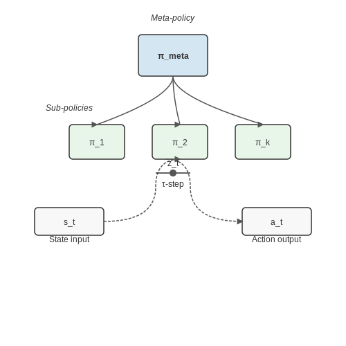
Hierarchical exploration strategies decompose the exploration problem into multiple levels of abstraction, enabling more efficient search in complex environments. At the highest level, a meta-policy selects among sub-policies, each responsible for exploration at different temporal or state abstractions. This structure allows the agent to reason about exploration at varying granularities, avoiding the inefficiencies of flat exploration.
Mathematical Formulation
Consider a hierarchical policy π consisting of a meta-policy πmeta and k sub-policies {π1, ..., πk}. The meta-policy selects sub-policies at intervals of τ steps:
where zt ∈ {1, ..., k} is the sub-policy index at time t. Each sub-policy then operates for τ steps:
The value of a hierarchical exploration strategy can be quantified through the mutual information between the sub-policy selection and the expected information gain:
where H denotes entropy and It represents the information gain at time t.
Meta-Exploration Strategies
Meta-exploration extends hierarchical approaches by learning the exploration strategy itself. The meta-learner optimizes an exploration objective over a distribution of tasks, enabling rapid adaptation to novel environments. Key approaches include:
- Gradient-Based Meta-Exploration: Uses meta-gradient descent to learn exploration parameters that generalize across tasks.
- Contextual Meta-Exploration: Employs contextual bandits at the meta-level to adapt exploration strategies based on environment characteristics.
- Memory-Augmented Meta-Exploration: Incorporates external memory to store and retrieve exploration strategies based on environment similarity.
Practical Implementation
Implementing hierarchical exploration requires careful design of the abstraction levels. A common approach uses:
class HierarchicalExploration:
    def __init__(self, num_sub_policies, meta_policy, sub_policies):
        self.num_sub_policies = num_sub_policies
        self.meta_policy = meta_policy  # Neural network
        self.sub_policies = sub_policies  # List of neural networks
        self.current_sub_policy = None
        self.steps_remaining = 0

    def select_action(self, state):
        if self.steps_remaining <= 0:
            # Sample new sub-policy
            policy_logits = self.meta_policy(state)
            self.current_sub_policy = tf.random.categorical(
                policy_logits, 1)[0, 0]
            self.steps_remaining = TAU  # Time horizon

        # Use current sub-policy
        action = self.sub_policies[self.current_sub_policy](state)
        self.steps_remaining -= 1
        return action
Applications in Real-World Systems
Hierarchical exploration has shown success in:
- Robotics: Where different levels can correspond to object manipulation vs. navigation strategies.
- Scientific Discovery: Meta-exploration accelerates the search for novel materials or chemical compounds.
- Game Playing: Agents learn exploration strategies transferable across different game levels or rule variations.
Performance Considerations
The effectiveness of hierarchical exploration depends on:
- The choice of temporal abstraction τ
- The diversity and specialization of sub-policies
- The meta-policy's ability to identify promising exploration directions
Empirical studies show that hierarchical approaches can reduce sample complexity by 2-10× compared to flat exploration in complex environments with sparse rewards.
4. Balancing Exploration in Deep Reinforcement Learning
4.1 Balancing Exploration in Deep Reinforcement Learning
The Exploration-Exploitation Tradeoff in Deep RL
In deep reinforcement learning (DRL), the exploration-exploitation dilemma is exacerbated by the high-dimensional state and action spaces typical of modern applications. Unlike tabular RL, where exploration can be systematically addressed (e.g., via ε-greedy or UCB), DRL requires more sophisticated strategies due to:
- Nonlinear function approximation: Neural networks generalize across states, making local exploration less effective.
- Correlated updates: Temporal difference learning with experience replay creates dependencies between sampled transitions.
- Delayed rewards: Sparse or deceptive reward signals in complex environments.
Intrinsic Motivation Methods
Intrinsic reward mechanisms augment the environmental reward rt with an exploration bonus it:
where β controls the exploration-exploitation balance. Common approaches include:
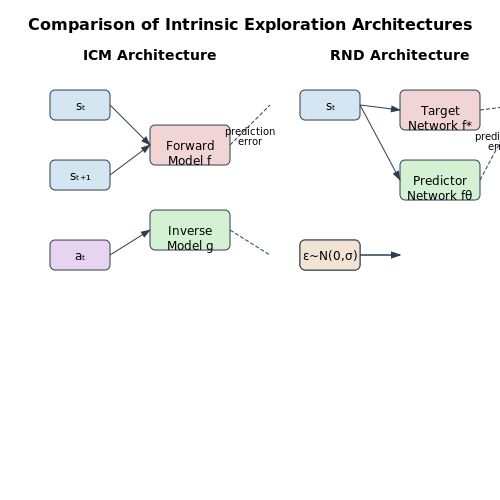
1. Curiosity-Driven Exploration (ICM)
Intrinsic Curiosity Module (ICM) trains an inverse dynamics model g and forward dynamics model f:
The exploration bonus is the prediction error of the forward model:
2. Random Network Distillation (RND)
RND uses two neural networks:
- A fixed random target network f*
- A trainable predictor network fθ
The intrinsic reward is the MSE between their outputs:
Noise-Based Exploration in Policy Gradients
For policy gradient methods, exploration is achieved through:
1. Parameter Space Noise
Additive Gaussian noise is applied to policy network weights:
where σ decays over time according to:
2. Action Space Noise (e.g., SAC)
Soft Actor-Critic (SAC) maximizes both reward and entropy:
where α is the temperature parameter controlling stochasticity.
Bayesian Deep RL Approaches
Bayesian methods quantify uncertainty in value estimates:
where κ governs exploration magnitude. Practical implementations include:
- Bootstrapped DQN: Multiple Q-heads with dropout
- Bayes-by-Backprop: Learned weight uncertainty
Empirical Considerations
Key practical challenges in DRL exploration:
- Memory-based methods: Episodic memory can prevent revisiting states (e.g., Go-Explore)
- Non-stationarity: Exploration strategies must adapt as the policy improves
- Scaling laws: Exploration bonuses must remain meaningful across different state visitation frequencies
4.2 Scalability and Computational Efficiency
Balancing exploration and exploitation in large-scale decision-making systems introduces computational challenges that grow exponentially with the state-action space. Traditional methods like ε-greedy or UCB become intractable in high-dimensional environments due to their linear dependence on the number of actions. For a problem with N actions, UCB requires maintaining and updating N confidence intervals, leading to O(N) space and time complexity per iteration.
Approximation Methods for Large Action Spaces
When exact computation is infeasible, function approximation techniques map actions to their estimated values via parametric models. The UCB objective can be reformulated using a neural network with parameters θ:
where Qθ(s,a) is a differentiable approximation of the action-value function. This reduces storage requirements from O(N) to O(d), where d is the number of network parameters. However, exploration now depends on the network's ability to generalize uncertainty estimates to novel actions.
Parallelization and Distributed Exploration
Thompson sampling naturally lends itself to parallel implementation through particle filtering. Each worker maintains an independent posterior sample, enabling simultaneous exploration of multiple promising regions. The computational cost scales as:
where P is the number of workers, K is the number of particles, and d3 comes from covariance matrix operations in Gaussian bandits. For deep variants, the cubic term becomes the cost of backpropagation through the network.
Sparse Approximation Techniques
In contextual bandits with infinite action spaces, kernel methods provide theoretical guarantees but suffer from O(t2) memory growth. Nyström approximation and random Fourier features reduce this to O(md) by projecting onto a fixed m-dimensional subspace:
where φi are the approximate feature maps. This enables UCB-style algorithms to run in sublinear time while preserving regret bounds.
Hierarchical Exploration Strategies
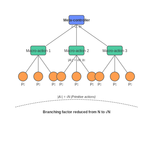
Multi-level architectures decompose the decision process into macro-actions and primitive actions. The hierarchy reduces the effective branching factor from N to √N at each level, transforming the complexity from exponential to polynomial. The meta-controller's exploration budget B follows:
where L is the hierarchy depth and bi is the budget per node at level i. This structure enables efficient exploration in domains like robotics and automated theorem proving.
Hardware-Aware Algorithm Design
Modern GPU/TPU architectures favor batched computation over sequential updates. Variants of UCB that process mini-batches of size M achieve O(1) amortized cost per decision by exploiting matrix operations:
where bold symbols denote batched vectors. This approach achieves 100-1000× speedups on accelerator hardware while maintaining identical regret bounds to sequential versions.
4.3 Common Pitfalls and How to Avoid Them
Overemphasis on Short-Term Rewards
A frequent mistake in exploration-exploitation trade-offs is myopic optimization, where algorithms prioritize immediate rewards over long-term gains. This often manifests in greedy policies that exploit known high-reward actions without sufficient exploration. The regret bound for such strategies grows linearly with time, violating the optimal logarithmic regret bound established by Lai and Robbins. To mitigate this, implement upper confidence bound (UCB) methods, where the action selection criterion balances estimated reward and uncertainty:
Here, c controls exploration intensity, while N_t(a) tracks action selection counts. This ensures systematic exploration of under-sampled actions.
Premature Convergence in Non-Stationary Environments
Static exploration strategies fail in dynamic environments where reward distributions drift over time. A classic example is epsilon-greedy policies with fixed ε, which continue exploring suboptimal actions even after environmental shifts. Adaptive methods like sliding-window UCB or discounted UCB address this by:
- Weighting recent observations more heavily
- Forgetting outdated samples exponentially: γt-kr_k where γ ∈ (0,1)
Curse of Dimensionality in Continuous Spaces
Discretization-based exploration becomes computationally intractable in high-dimensional action spaces. Thompson sampling with Bayesian neural networks offers a scalable alternative by maintaining posterior distributions over Q-values. The key steps involve:
- Sampling model parameters θ ~ p(θ|D)
- Selecting actions maximizing Qθ(s,a)
- Updating posteriors via variational inference
Misalignment Between Exploration and Objective
Optimizing for pure information gain (e.g., maximum entropy exploration) may diverge from task objectives. In robotics, this manifests as aimless wandering instead of goal-directed behavior. Hybrid intrinsic-extrinsic reward functions solve this:
where I(·) denotes mutual information and β balances curiosity with task rewards.
Numerical Instability in Variance Estimates
Variance-based exploration (e.g., Bootstrapped DQN) suffers from erratic updates when sample counts are low. Numerical stabilization techniques include:
- Adding small ε to denominator terms
- Clipping advantage estimates
- Using pseudocounts for unvisited states
Hyperparameter Sensitivity
The performance of exploration strategies like Boltzmann exploration critically depends on temperature parameter τ:
Automated adaptation methods include:
- Annealing schedules: τ = τ0e-kt
- Bandit meta-learners optimizing τ online
- Gradient-based tuning with auxiliary objectives
5. Regret Analysis and Performance Benchmarks
Regret Analysis and Performance Benchmarks
Foundations of Regret in Multi-Armed Bandits
Regret quantifies the difference between the cumulative reward of an optimal strategy and the actual reward obtained by a learning algorithm. In the stochastic multi-armed bandit (MAB) setting with K arms, the expected cumulative regret RT after T rounds is defined as:
where μ* is the mean reward of the optimal arm and μat is the mean reward of the arm selected at time t. For algorithms like UCB1 and Thompson Sampling, regret bounds are typically derived using concentration inequalities and martingale analysis.
Lower Bounds and Optimality
Lai and Robbins (1985) established a fundamental lower bound for regret in stochastic bandits. For any consistent policy (where RT grows sublinearly), the asymptotic regret must satisfy:
where KL denotes the Kullback-Leibler divergence. Algorithms achieving this bound are called asymptotically optimal. The UCB1 algorithm, for instance, achieves:
where Δi = μ* - μi is the suboptimality gap.
Non-Stationary and Adversarial Regret
In non-stationary environments where reward distributions change over time, dynamic regret measures performance against a time-varying comparator. For adversarial bandits, the pseudo-regret is defined as:
The EXP3 algorithm achieves O(√(KT log K)) regret in this setting. Recent advances like the Tsallis-INF algorithm improve this to O(√(KT)) without logarithmic factors.
Empirical Evaluation Metrics
Beyond theoretical bounds, practical benchmarks evaluate:
- Cumulative regret curves showing RT vs T
- Time to threshold: Steps needed to achieve a target regret level
- Arm selection frequency: Distribution over optimal/suboptimal pulls
- Adaptation speed in non-stationary environments
Standard testbeds include:
- Stationary Gaussian/Bernoulli bandits with varying gap sizes
- Abrupt/gradual change scenarios for non-stationary testing
- Adversarial reward sequences with bounded variation
Advanced Techniques in Regret Analysis
Modern approaches leverage:
- Variance-adaptive bounds that depend on reward variances rather than worst-case gaps
- High-probability regret guarantees beyond expectation
- Problem-dependent vs problem-independent bounds
- Gradient-based analysis for linear and contextual bandits
For linear bandits with d-dimensional features, the optimal regret scales as O(d√T), achieved by algorithms like LinUCB. The exact bound depends on the action set geometry:
where C depends on the reward noise and feature norm constraints.
5.2 Empirical Comparison of Methods
Performance Metrics in Exploration-Exploitation
The efficacy of exploration-exploitation strategies is typically evaluated using three key metrics: cumulative regret, simple regret, and convergence rate. Cumulative regret measures the total loss incurred by not always selecting the optimal action up to time T:
where μ* is the expected reward of the optimal action and μa_t is the reward of the chosen action at time t. Simple regret, in contrast, evaluates the quality of the final recommended action after T rounds. The convergence rate quantifies how quickly an algorithm reduces its regret over time, often analyzed using big-O notation.
Bandit Algorithms: Finite-Armed Case
In stochastic bandits with K arms, UCB1 achieves logarithmic regret:
where Δi represents the suboptimality gap for arm i. Thompson sampling, while Bayesian in nature, demonstrates comparable asymptotic performance but often exhibits better empirical performance in early rounds due to its probabilistic exploration.
Contextual Bandits and High-Dimensional Spaces
For contextual bandits with d-dimensional features, LinUCB achieves regret:
where the Õ notation hides logarithmic factors. Neural network-based approaches like NeuralUCB can achieve sublinear regret in certain function classes, but their empirical performance heavily depends on the quality of uncertainty quantification in the neural network's predictions.
Deep Exploration in RL
In deep reinforcement learning, Bootstrapped DQN demonstrates superior empirical performance over ε-greedy methods in environments requiring deep exploration, such as Montezuma's Revenge. The key advantage stems from maintaining multiple value function hypotheses, enabling systematic exploration of diverse trajectories. Quantitatively, Bootstrapped DQN achieves up to 5× higher rewards than ε-greedy baselines in hard exploration tasks.
Bayesian Optimization Benchmarks
When comparing Gaussian Process Upper Confidence Bound (GP-UCB) to Expected Improvement (EI) on synthetic functions:
where γT is the maximum information gain after T iterations. EI often outperforms GP-UCB in low-dimensional spaces (d < 5), while GP-UCB shows better robustness in higher dimensions. Recent hybrid approaches like Predictive Entropy Search demonstrate 15-30% faster convergence on benchmark functions like Hartmann-6 compared to pure GP-UCB.
Non-Stationary Environments
For abruptly changing environments, Discounted UCB achieves:
where ΓT measures the total variation in reward distributions. Sliding-Window Thompson Sampling shows particular empirical strength in advertising applications, reducing regret by 20-40% compared to stationary approaches when ad click-through rates change weekly.
5.3 Choosing the Right Strategy for Your Problem
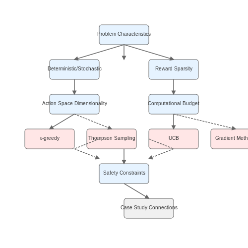
The trade-off between exploration and exploitation is problem-dependent, requiring careful consideration of the environment's structure, reward dynamics, and computational constraints. The optimal strategy balances short-term gains with long-term learning, influenced by factors such as stochasticity, non-stationarity, and partial observability.
Problem Characteristics
The nature of the environment dictates the appropriate strategy. In deterministic settings with known reward distributions, pure exploitation suffices. However, in stochastic or non-stationary environments, exploration becomes crucial to adapt to changing dynamics. Key considerations include:
- Reward sparsity: Sparse rewards necessitate extensive exploration to discover meaningful signals.
- Action space dimensionality: High-dimensional spaces require efficient exploration methods like intrinsic motivation or curiosity-driven learning.
- Episodic vs. continuing tasks: Episodic tasks may tolerate more exploration early, while continuing tasks demand persistent balance.
Algorithm Selection Framework
The choice between ε-greedy, Thompson sampling, UCB, or Boltzmann exploration depends on mathematical properties of the problem. For bandit problems with independent arms, Thompson sampling provides Bayesian optimality:
where θ represents the unknown parameters and D the observed data. For MDPs with state dependencies, UCB-based methods offer regret bounds:
where c controls exploration intensity and N_t(a) counts selections of action a.
Practical Implementation Considerations
Real-world deployment introduces additional constraints:
- Computational budget: Thompson sampling requires posterior updates, while ε-greedy has constant-time complexity.
- Safety constraints: Risk-sensitive domains may employ constrained exploration or conservative updating.
- Non-stationarity detection: Sliding window or discount factors adapt to changing environments.
Case Study: Recommendation Systems
Modern recommender systems exemplify adaptive strategy selection. A hybrid approach might combine:
- Thompson sampling for new item exploration
- LinUCB for contextual bandit scenarios
- ε-decay for gradual transition to exploitation
The optimal mixture depends on user engagement metrics and item turnover rates, often implemented as a meta-learner that dynamically adjusts strategy weights based on real-time performance.
Advanced Techniques
Recent advances incorporate deep learning for strategy adaptation:
where f_φ is a neural network that learns exploration bonuses end-to-end. This approach automatically adapts exploration strategies to the problem's latent structure.
6. Foundational Papers and Key Research
6.1 Foundational Papers and Key Research
- Exploration and exploitation: Which research strategy are you better at ... — Abstract. This study quantifies and analyzes the individual-level abilities of scientists utilizing either an exploration or an exploitation strategy. Specifically, we present a Research Strategy Q model, which untangles the coupling effect of scientists' research ability (Qα) and research strategy ability (Eαπ) on research performance. Qα indicates scientists' fundamental ability to ...
- Revisiting the exploration-exploitation behavior of scholars' research ... — In this paper, we further divide exploration-exploitation behavior into five fine-grained research strategies. The goal of this study is to quantitatively analyze the relationship between scientists' research performance and their preference for different research strategies, and examine the evolution of the preference.
- 1 Introduction — How does varying the balance between exploration and exploitation impact decision quality? 1.1 Summary of Results and Contributions Modeling contributions. In this paper, we introduce a novel model that bridges algorithmic and behavioral modeling to shed light on the dynamic interplay between exploration and exploitation.
- Managing tensions between exploitative and exploratory innovation ... — A long tradition of research in organization theory suggests that, at firm level, pursuing exploration and exploitation goals simultaneously may require structures and actions that are fundamentally at odds, making it difficult to pursue both simultaneously without changing organizational processes (March 1991; Tushman and O'Reilly, 1996).
- PDF Exploration vs. Exploitation: Navigating Consumer Behavior ... - SSRN — behaviors—exploration, where they seek out new conten engaging with content they have already found enjoyable. This dynamic presents a key challenge of accurately identifying and understanding consumers' exploration-exploitation states because effective digital strategies, such as consumer engagement, heavily dep
- PDF An Active Learning Perspective on Exploration in Reinforcement Learning — Balancing this trade-off is called the exploration vs. exploitation problem, and is the primary focus of this thesis. The work is organized around three related research questions. Exploration algorithms have proliferated in the last few years. There are differences in the way exploration techniques create exploratory behavior.
- Fundamental Tradeoffs Between Exploration and Exploitation Search ... — The hybridization method is intended to upgrade the exploration and exploitation performance by improving their functionality through combination with other search techniques. The methods are divided into different control strategies, including integrative and collaborative hybrid.
- PDF Exploration-Exploitation Trade-off Approaches in Multi-Armed Bandit — recently gained significant attention due to numerous applications. In Multi-armed Bandit, an agent faces the central challenge of choosing exploitation of its belief to hopefully gain a high reward and exploration to improve its knowledge of the environment, and any good strategy has to efficiently balance between the two actions. Being particularly interested in the Bernoulli reward signal ...
- PDF Exploration vs. Exploitation: An Empirical Test of the Impact of ... — In this paper, we used the exploration vs. exploitation construct to operationalize the technological innovation strategy of firms and examined their impacts on firm perfor mance.
- Exploration vs. Exploitation in Differential Evolution — This paper explores the balance between exploration and exploitation within the framework of Differential Evolution, a prominent evolutionary computation algorithm. It discusses the implications of this balance on optimization problems, emphasizing the need for adaptive strategies that can efficiently navigate complex solution spaces. The findings aim to improve decision-making processes in ...
6.2 Recommended Books and Surveys
- Fundamental Tradeoffs Between Exploration and Exploitation Search ... — 2.1.2 Tradeoff Exploration-Exploitation. Both strategies of exploration and exploitation need to be balanced to achieve a good performance of the optimization algorithm (Yang 2014; Salleh et al. 2018). The idea of achieving a good balance is still in open problem (Yang 2014) and the question of balancing between both components is recurrent ...
- Managing tensions between exploitative and exploratory innovation ... — 6 (2) 6 (6) 3 (1) 1 (1) 18: Interview dates: December 08, 2017 February 23, 2018: December 15, 2017: ... The first phase corresponds to the search and survey of advanced innovations: S Corp has not yet defined a project and they do not know what they need although they do know that something needs investigating. ... Exploration vs. exploitation ...
- PDF Exploration vs. Exploitation: Reducing Uncertainty in Operational ... — Exploration vs. Exploitation: Reducing Uncertainty in Operational Problems by Yaron Shaposhnik B.Sc., Technion Israel Institute of Technology (2006) M.Sc., Technion Israel Institute of Technology (2011) Submitted to the Sloan School of Management in partial ful llment of the requirements for the degree of Doctor of Philosophy in Operations Research
- Exploration versus exploitation decisions in the human brain: A ... — The exploration-exploitation trade-off offers an important lens through which to study the behavioural and neural development of biological systems. In humans, the focus of the current review, this trade-off has been linked to reward and affective drives and associated neural circuitry (Cohen, et al., 2007).
- Exploration and exploitation: Which research strategy are you better at ... — Abstract. This study quantifies and analyzes the individual-level abilities of scientists utilizing either an exploration or an exploitation strategy. Specifically, we present a Research Strategy Q model, which untangles the coupling effect of scientists' research ability (Qα) and research strategy ability (Eαπ) on research performance. Qα indicates scientists' fundamental ability to ...
- Exploration in deep reinforcement learning: A survey — The exploration-exploitation dilemma is an ongoing research topic not only in reinforcement learning but also in a general problem. Most current exploration approaches have a built-in solution to exploration-exploitation, but not all methods do. This is particularly true in goal-based methods that rely on hand-designed solutions.
- PDF Exploration vs. Exploitation: An Empirical Test of the Impact of ... — The exploration vs. exploitation distinction has been extensively used in the organizational learning literature (see e.g., March, 1991; Levinthal & March, 1993). The need to balance
- (PDF) A Behavioral Model for Exploration vs. Exploitation: Theoretical ... — Author: A Behavioral Mo del for Exploration vs. Exploitation Article submitted to Management Science ; manuscript no. 7 policy of the DM is go verned by a mapping from a historical path h t − 1 ...
- Improve IT Sustainability with IT Technology - Comparison ... - Springer — 3.2 Exploration vs Exploitation of Technologies. The exploit approach is based on the "never change a running system" strategy. In this case a working and running setup is not touched as it is not needed or it is adjusted with minimal change as possible.
- PDF The Path Forward: A Primer for Reinforcement Learning - Stanford University — was not a general strategy, and anyway it was not how people played chess. These researchers wanted methods based on human input to win and were disappointed when they did not. A similar pattern of research progress was seen in computer Go, only delayed by a further 20 years. Enormous initial efforts went into avoiding search by
6.3 Open-source Implementations and Toolkits
- D5.3 - Exploitation Strategy and Roadmap | PDF | Cryptocurrency - Scribd — 6. Contributions to open-source projects and standardisation; through publication of open-source toolkits and participation in relevant standardisation groups. We have created the following exploitation strategy, in order to help each partner with formulating a specific exploitation plan. These respective plans will loosely be organized along ...
- Impacts of strategic exploitation and exploration on firms' survival ... — To observe the efficacy of only adopting exploitation or exploration or of adopting ambidexterity, the ratio of the number of survived firms to the number of delisted firms in each strategy was computed. The ratios were 10.44, 2.64, and 2.11 for the exploitation, exploration, and ambidexterity strategies, respectively.
- Fundamental Tradeoffs Between Exploration and Exploitation Search ... — 2.1.2 Tradeoff Exploration-Exploitation. Both strategies of exploration and exploitation need to be balanced to achieve a good performance of the optimization algorithm (Yang 2014; Salleh et al. 2018). The idea of achieving a good balance is still in open problem (Yang 2014) and the question of balancing between both components is recurrent ...
- PDF An Active Learning Perspective on Exploration in Reinforcement Learning — trade-off is called the exploration vs. exploitation problem, and is the primary ... and has been a reliable source of guidance throughout the year. I am thankful to Jim for encouraging me ... 5.2 Implementations of exploration methods from each category46
- Knowledge exploitation, knowledge exploration, and competency trap ... — It is no surprise that knowledge exploitation and knowledge exploration have become the consistent theme in organizational learning literature. Strategy and organization theorists have similarly observed the dynamic capabilities anchored in a firm's ability to simultaneously exploit current technologies and resources to secure efficiency ...
- Managing tensions between exploitative and exploratory innovation ... — A long tradition of research in organization theory suggests that, at firm level, pursuing exploration and exploitation goals simultaneously may require structures and actions that are fundamentally at odds, making it difficult to pursue both simultaneously without changing organizational processes (March 1991; Tushman and O'Reilly, 1996).This dilemma is particularly important in product ...
- PDF Exploration-Exploitation Trade-off Approaches in Multi-Armed Bandit — the central challenge of choosing exploitation of its belief to hopefully gain a high reward and exploration to improve its knowledge of the environment, and any good strategy has to efficiently balance between the two actions. Being particularly interested in the Bernoulli reward signal, in
- Dealing with uncertainty: balancing exploration and exploitation in ... — Reinforcement learning (RL) is a core topic in machine learning and is concerned with sequential decision-making in an uncertain environment. Two key concepts in RL are exploration, which consists of learning via interactions with an unknown environment, and exploitation, which consists of optimizing the objective function given accumulated information.
- PDF Exploration vs. Exploitation: Reducing Uncertainty in Operational ... — Exploration vs. Exploitation: Reducing Uncertainty in Operational Problems by Yaron Shaposhnik B.Sc., Technion Israel Institute of Technology (2006) M.Sc., Technion Israel Institute of Technology (2011) Submitted to the Sloan School of Management in partial ful llment of the requirements for the degree of Doctor of Philosophy in Operations Research
- Meta-Learning of Exploration/Exploitation Strategies: The Multi-Armed ... — We develop a meta-learning framework for simple regret minimization in bandits. In this framework, a learning agent interacts with a sequence of bandit tasks, which are sampled i.i.d.\ from an ...