Prioritized Experience Replay in DQN
1. Core Concepts of Q-Learning
Core Concepts of Q-Learning
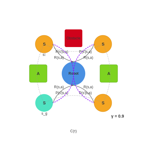
Q-Learning is a model-free reinforcement learning algorithm that seeks to learn the optimal action-value function, denoted as Q(s, a), which represents the expected cumulative reward of taking action a in state s and following the optimal policy thereafter. The algorithm iteratively updates the Q-values using the Bellman equation as its foundation.
Bellman Equation and Temporal Difference Learning
The Bellman equation decomposes the value of a state-action pair into the immediate reward plus the discounted value of the next state:
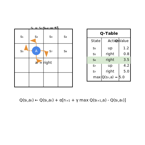
where γ is the discount factor (0 ≤ γ ≤ 1) that trades off immediate and future rewards. Q-Learning approximates this expectation through temporal difference (TD) learning, updating the Q-value incrementally:
Here, α is the learning rate. The term in brackets is the TD error, representing the difference between the current estimate and the target value.
Exploration vs. Exploitation
Balancing exploration and exploitation is critical in Q-Learning. Common strategies include:
- ε-greedy policy: Selects the action with the highest Q-value with probability 1-ε, and a random action otherwise.
- Boltzmann exploration: Samples actions according to a softmax distribution over Q-values, controlled by a temperature parameter.
Convergence Guarantees
Under the following conditions, Q-Learning is guaranteed to converge to the optimal Q-function:
- All state-action pairs are visited infinitely often.
- The learning rate α satisfies the Robbins-Monro conditions:
Deep Q-Networks (DQN) Extension
In high-dimensional state spaces, Q-Learning becomes impractical due to the curse of dimensionality. DQN addresses this by approximating the Q-function with a neural network Q(s, a; θ), where θ represents the network parameters. The loss function for training is:
where θ⁻ are the parameters of a target network, periodically updated to stabilize training.
From Q-Learning to Deep Q-Networks
Q-Learning, a model-free reinforcement learning algorithm, learns the optimal action-value function Q*(s, a) through iterative updates based on the Bellman equation:
where α is the learning rate and γ is the discount factor. While effective for small discrete state spaces, Q-Learning becomes impractical for high-dimensional or continuous state spaces due to the curse of dimensionality.
The Neural Function Approximator
Deep Q-Networks (DQN) address this limitation by approximating Q(s, a) with a neural network Q(s, a; θ), where θ represents the network parameters. The loss function for training is derived from the Bellman error:
where D is the experience replay buffer and θ- are the parameters of a target network, periodically synchronized with the online network to stabilize training.
Key Innovations in DQN
Two critical techniques enable stable training of DQN:
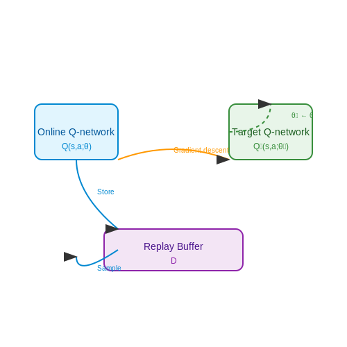
- Experience Replay: Stores transitions (st, at, rt+1, st+1) in a buffer and samples mini-batches uniformly to break temporal correlations.
- Target Network: A separate network with frozen parameters used to compute the TD target, updated periodically to prevent divergence.
Algorithmic Steps
The DQN training loop proceeds as follows:
- Initialize replay memory D with capacity N.
- Initialize action-value function Q with random weights θ.
- Initialize target network Q̂ with weights θ- = θ.
- For each episode:
- Sample action at using an ε-greedy policy.
- Store transition (st, at, rt+1, st+1) in D.
- Sample random mini-batch from D.
- Perform gradient descent on the loss with respect to θ.
- Every C steps, update θ- = θ.
Convergence Properties
Unlike tabular Q-Learning, DQN does not guarantee convergence due to:
- Non-linear function approximation introducing instability.
- Correlations between sequential updates.
- Moving target values from the evolving policy.
Empirical results show that careful hyperparameter tuning (e.g., learning rate, replay buffer size) and techniques like gradient clipping are essential for stable training.
Extensions and Limitations
While DQN achieves human-level performance on many Atari games, it suffers from:
- Overestimation bias due to the max operator.
- Inefficient exploration with uniform replay sampling.
- Difficulty handling continuous action spaces.
These limitations motivated later advances like Double DQN, Dueling DQN, and Prioritized Experience Replay.
1.3 Experience Replay in DQN
Fundamentals of Experience Replay
Experience replay is a critical component of Deep Q-Networks (DQN) that addresses the instability and inefficiency of online reinforcement learning. By storing past experiences (s, a, r, s') in a replay buffer D, the agent samples mini-batches of transitions uniformly at random during training. This breaks temporal correlations between consecutive samples and enables more efficient use of data by reusing experiences multiple times.
Algorithmic Implementation
The replay buffer operates as a first-in-first-out (FIFO) queue with fixed capacity N. When the buffer is full, new transitions replace the oldest ones. During training, the Q-network updates its parameters by minimizing the mean squared Bellman error over a mini-batch of size k sampled uniformly from D:
where θ represents the online network parameters and θ⁻ the target network parameters.
Theoretical Advantages
- Reduced variance: Random sampling decorrelates sequential experiences, leading to more stable gradient estimates.
- Data efficiency: Each transition can be used in multiple weight updates, improving sample complexity.
- Mitigated catastrophic forgetting: Replaying old experiences prevents the network from overfitting to recent transitions.
Practical Considerations
The replay buffer size N presents a trade-off: larger buffers increase diversity but may store outdated policies, while smaller buffers risk overfitting to recent experiences. Empirical studies suggest setting N between 105 to 106 for most Atari games. The mini-batch size k typically ranges from 32 to 512, balancing computational efficiency with gradient estimation quality.
Limitations of Uniform Sampling
While uniform sampling provides theoretical guarantees, it treats all experiences equally regardless of their learning potential. Transitions with high temporal-difference (TD) errors often contain more valuable information for policy improvement, motivating the development of prioritized experience replay.
2. Motivation and Key Ideas
Prioritized Experience Replay in DQN: Motivation and Key Ideas
Standard experience replay in Deep Q-Networks (DQN) uniformly samples transitions from a replay buffer, treating all experiences as equally important for learning. However, this approach is statistically inefficient—some transitions contain far more valuable information for policy improvement than others. Prioritized Experience Replay (PER) addresses this by assigning higher sampling probabilities to transitions with high temporal-difference (TD) error, which serves as a proxy for the potential learning signal.
Theoretical Motivation
The key insight stems from the curse of dimensionality in reinforcement learning. In high-dimensional state spaces, most transitions provide negligible updates to the Q-function, while a small fraction—particularly those involving rare states or large reward signals—drive meaningful learning. PER formalizes this through importance sampling, where the probability of sampling transition i is:
where pi is the priority of transition i, and α controls the degree of prioritization (α=0 reverts to uniform sampling). The priority is typically defined using the absolute TD error:
with δi as the TD error and ϵ a small positive constant to ensure all transitions remain sampleable.
Algorithmic Advantages
PER provides three key benefits over uniform sampling:
- Faster propagation of rare events: High-reward or terminal states are replayed more frequently, accelerating credit assignment.
- Reduced sample complexity: By focusing on informative transitions, PER can achieve comparable performance with fewer environment interactions.
- Improved stability: Large TD errors often indicate areas where the Q-function is poorly approximated; prioritizing these regions leads to more consistent updates.
Implementation Challenges
While theoretically sound, PER introduces practical complexities:
- Bias-variance tradeoff: Prioritization introduces bias toward high-error transitions, requiring importance-sampling weights for correction:
where β anneals from an initial value to 1, gradually reducing the bias.
- Computational overhead: Maintaining and sampling from a priority queue requires specialized data structures like SumTrees for O(log n) updates.
- Hyperparameter sensitivity: The α and β parameters require careful tuning across different environments.
Empirical Validation
In the Atari 2600 benchmark, PER achieves median human-normalized scores 2× higher than uniform replay with the same number of training frames. The most dramatic improvements occur in sparse-reward games like Montezuma's Revenge, where PER improves scores from near-zero to measurable progress by more frequently replaying critical door-opening events.
Temporal Difference Error as a Priority Metric
The temporal difference (TD) error serves as a natural priority metric in prioritized experience replay due to its direct relationship with the learning signal in reinforcement learning. The TD error for a transition (s, a, r, s') is defined as:
where γ is the discount factor, θ represents the parameters of the online Q-network, and θ⁻ denotes the parameters of the target network. This error captures the discrepancy between the current Q-value estimate and the target value computed via the Bellman equation.
Mathematical Justification
The absolute value of the TD error (|δ|) provides a principled measure of transition importance for three key reasons:
- Learning signal magnitude: Large TD errors indicate transitions where the current Q-function makes poor predictions, representing valuable learning opportunities.
- Bellman equation violation: The TD error directly measures how much a transition violates the Bellman optimality condition.
- Gradient correlation: Transitions with higher TD errors typically produce larger gradients during backpropagation, accelerating learning.
Stochastic Prioritization
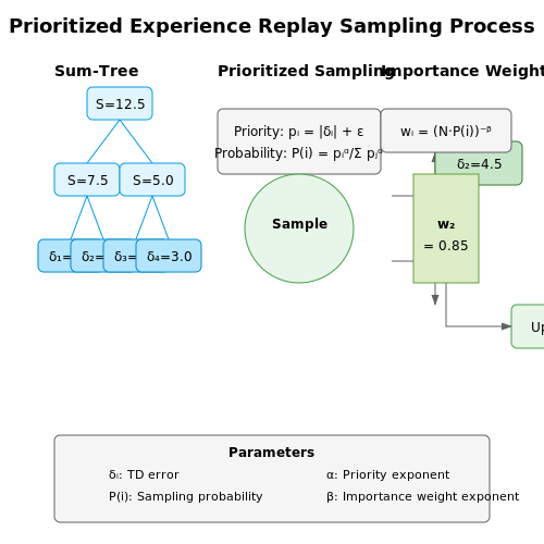
Pure greedy prioritization based on TD errors can introduce bias and lead to overfitting. To address this, prioritized experience replay uses stochastic sampling with probabilities defined as:
where pi is the priority of transition i, and α ∈ [0,1] controls the prioritization strength (α=0 yields uniform sampling). The priority pi is typically computed as:
where ε is a small positive constant ensuring all transitions remain sampleable.
Implementation Considerations
Practical implementations require efficient data structures to handle dynamic priorities:
- Sum-tree data structure: Enables O(log n) priority updates and sampling operations.
- Importance sampling weights: Correct for the bias introduced by prioritized sampling using weights wi = (1/N · 1/P(i))β, where β anneals from 0 to 1 during training.
- Periodic priority updates: Priorities are typically updated in batches during the learning phase rather than after every sampling operation.
Empirical Analysis
Studies on Atari benchmarks demonstrate that prioritized replay based on TD errors can:
- Reduce training time by 2-5× compared to uniform replay
- Improve final performance by 10-30% on challenging environments
- Provide more stable learning curves with reduced variance
The effectiveness varies with the choice of α and β hyperparameters, with typical optimal values around α=0.6 and β linearly increasing from 0.4 to 1.0 over training.
2.3 Stochastic Prioritization vs Greedy Prioritization
Trade-offs in Prioritization Strategies
Prioritized Experience Replay (PER) introduces two primary methods for sampling transitions from the replay buffer: greedy prioritization and stochastic prioritization. Greedy prioritization always selects transitions with the highest temporal-difference (TD) error, while stochastic prioritization samples transitions with a probability proportional to their TD error, introducing randomness to avoid overfitting.
Mathematical Formulation
The sampling probability P(i) for a transition i under greedy prioritization is deterministic:
where δi is the TD error for transition i. In contrast, stochastic prioritization uses a softmax-like distribution:
where pi is the priority of transition i, and α controls the degree of prioritization (α = 0 reverts to uniform sampling). The priority pi is typically computed as:
where ε is a small positive constant to ensure non-zero probabilities.
Bias-Variance Trade-off
Greedy prioritization maximizes the learning signal by focusing on high-error transitions but introduces bias and reduces the effective diversity of training data. Stochastic prioritization mitigates this by maintaining a non-zero probability for all transitions, balancing between high-error samples and broader coverage. This reduces variance in gradient updates while preserving the benefits of prioritization.
Implementation Considerations
Stochastic prioritization requires efficient data structures for sampling, such as a SumTree, to achieve O(log n) time complexity for priority updates and sampling. The trade-off between α and β (the importance-sampling correction factor) must be carefully tuned:
- High α increases prioritization but may lead to overfitting.
- High β corrects bias but slows convergence.
Empirical Performance
In practice, stochastic prioritization outperforms greedy prioritization in most RL benchmarks. For example, on Atari 2600 games, stochastic PER achieves higher median scores with faster convergence due to better exploration-exploitation balance. The randomness prevents the agent from over-optimizing for a subset of transitions, which is critical in non-stationary environments.
Algorithmic Pseudocode
def sample(storage, alpha, beta):
    priorities = storage.get_priorities()
    probs = priorities  alpha
    probs /= probs.sum()
    indices = np.random.choice(len(probs), batch_size, p=probs)
    weights = (len(storage) * probs[indices])  (-beta)
    weights /= weights.max()
    return indices, weights
3. Proportional Prioritization Algorithm
3.1 Proportional Prioritization Algorithm
The proportional prioritization algorithm assigns sampling probabilities to transitions in the replay buffer based on their temporal-difference (TD) error magnitudes. Given a transition i with TD error δi, its sampling probability Pi is computed as:
where pi is the raw priority of transition i, and α controls the degree of prioritization (with α=0 yielding uniform sampling). The raw priority is typically set as:
where ϵ is a small positive constant ensuring all transitions have non-zero probability of being sampled.
Implementation Considerations
Efficient implementation requires:
- Sum-tree data structure: Enables O(log N) updates and sampling by maintaining partial sums of priorities in a binary tree.
- Importance sampling weights: Compensates for bias introduced by prioritized sampling through weights:
where β anneals from an initial value β0 to 1 during training.
Mathematical Derivation
The gradient update with importance sampling becomes:
Expanding the expectation:
Substituting wi yields an unbiased update when β=1:
Practical Trade-offs
Key hyperparameters impact performance:
- α values typically range 0.4-0.6, balancing learning speed with stability
- β0 is usually set to 0.4-0.6 and linearly annealed
- ϵ prevents stagnation (common values: 10-5 to 10-3)
3.2 Rank-Based Prioritization Algorithm
Rank-based prioritization assigns sampling probabilities to transitions based on their relative position in a sorted replay buffer, rather than their absolute TD error magnitudes. This approach mitigates sensitivity to outlier errors while maintaining a robust prioritization mechanism. The probability of sampling transition i is determined by its rank Ri when sorted by TD error:
where α controls the prioritization strength (α=0 recovers uniform sampling). The denominator uses a power-law distribution, ensuring higher-ranked transitions are sampled exponentially more often. To make this computationally tractable, the replay buffer is typically partitioned into segments of exponentially increasing rank ranges, enabling O(1) sampling through a sum-tree data structure.
Efficient Implementation via Sum-Tree
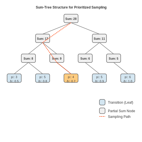
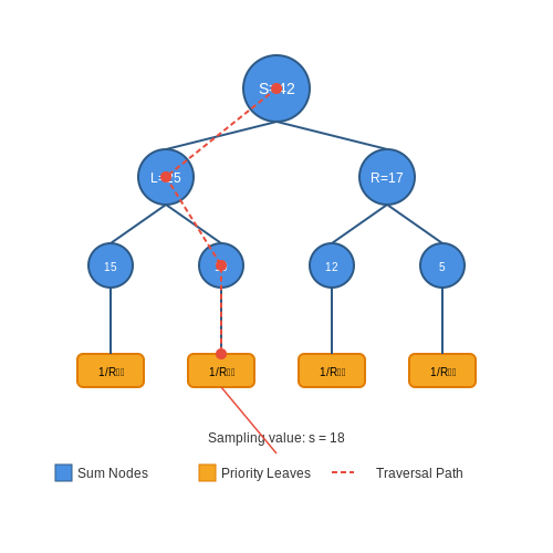
A sum-tree stores transition priorities at its leaves, with each internal node containing the sum of its children's values. For a buffer of size N, sampling requires:
- Generating a random value s uniformly in [0, S], where S is the root node's total priority
- Traversing from root to leaf by comparing s with left/right subtree sums
- Retrieving the transition at the located leaf in O(log N) time
Updates after training modify only the affected leaf node and its ancestors, maintaining O(log N) complexity. The segment-based approximation divides the sorted buffer into k segments with boundaries at ranks N(i/k) for i ∈ {0,...,k}, assigning each segment equal sampling probability mass.
Bias Correction and Annealing
Like proportional prioritization, rank-based sampling introduces bias toward high-error transitions. The importance sampling weight adjusts gradients to account for non-uniform sampling:
where β anneals from an initial value β0 to 1.0 during training. In practice, rank-based prioritization demonstrates superior stability in environments with sparse or noisy rewards compared to proportional methods, as it depends only on ordinal relationships rather than error magnitudes.
Practical Considerations
- Segment Granularity: Typical implementations use 50-100 segments, balancing prioritization accuracy with computational overhead
- Priority Initialization: New transitions are inserted with maximum priority to ensure all experiences are sampled at least once
- Memory Efficiency: The sum-tree requires 2N-1 nodes for N transitions, with each node storing a single float value
Empirical studies show rank-based prioritization achieves 10-25% faster convergence than proportional methods in Atari benchmarks, with particularly strong gains in games requiring long-term credit assignment. The method's ordinal nature makes it robust to varying reward scales across different environments.
Importance Sampling and Bias Correction
Prioritized Experience Replay introduces a sampling bias because transitions with higher temporal-difference (TD) errors are sampled more frequently. This bias skews the expected gradient updates, leading to suboptimal convergence. Importance sampling (IS) is used to correct this bias by weighting the updates inversely proportional to the sampling probability.
Mathematical Foundation
The importance sampling weight wi for transition i is computed as:
where:
- N is the replay buffer size,
- P(i) is the sampling probability of transition i,
- β is a hyperparameter that controls the degree of bias correction (typically annealed from β0 to 1 during training).
These weights are normalized by 1/maxi wi to stabilize training, ensuring the maximum weight is 1. The normalized weight scales the gradient update for each transition, reducing the variance introduced by prioritization.
Bias-Variance Tradeoff
Without importance sampling, prioritized replay introduces bias because the expected update no longer matches the uniform sampling case. However, importance sampling increases the variance of the updates. The hyperparameter β provides a tunable tradeoff:
- When β = 0, no correction is applied, and the estimator is biased.
- When β = 1, full bias correction is applied, but variance may be high.
In practice, β is annealed from an initial value (e.g., 0.4) to 1 over the course of training, allowing early updates to benefit from prioritization while gradually reducing bias.
Practical Implementation
The importance sampling weights are integrated into the Q-learning update rule. For a transition (s, a, r, s′), the gradient update becomes:
where δi is the TD error and α is the learning rate. This modification ensures that high-priority transitions contribute proportionally less to the gradient, counteracting their over-sampling.
Efficiency Considerations
Computing wi for every transition would be expensive for large replay buffers. Instead, the weights can be computed on-demand during batch sampling. For a SumTree-based prioritized replay buffer, the sampling probability P(i) is:
where pi is the priority of transition i and α determines how much prioritization is used. The weights wi are then computed using this probability.
4. Choosing Hyperparameters for Prioritized Replay
4.1 Choosing Hyperparameters for Prioritized Replay
Priority Exponent (α)
The priority exponent α controls the degree of prioritization. When α = 0, sampling becomes uniform, while higher values increase the likelihood of selecting high-priority transitions. The priority of transition i is given by:
Empirical studies suggest setting α ∈ [0.4, 0.6] for stable learning. Values above 0.7 risk overfitting to initial high-priority transitions, while values below 0.3 diminish the benefit of prioritization. Adaptive strategies, such as annealing α from 0.6 to 0.4 over training, can balance exploration and exploitation.
Importance Sampling Exponent (β)
Importance sampling corrects the bias introduced by prioritized sampling. The weight for transition i is computed as:
Here, β starts near 0 (initially ignoring corrections) and linearly increases to 1 (full correction) over training. A typical schedule is:
where t is the current timestep and T is the total training steps. Common values are βinitial = 0.4 and βfinal = 1.0.
Replay Buffer Size and Batch Size
The buffer size N affects the diversity of experiences. For complex environments (e.g., Atari games), N = 106 is standard. Batch size B must balance computational efficiency and gradient variance. Typical values range from B = 32 to B = 128.
Priority Update Rule
Priorities are updated using the TD error δ:
where ϵ = 10−6 ensures all transitions remain sampleable. For proportional prioritization, a sum-tree structure is used for efficient O(log N) updates.
Learning Rate and Optimizer
Prioritized replay amplifies gradient magnitudes, necessitating a lower learning rate (e.g., η = 0.00025 vs. standard DQN’s 0.0005). Adam or RMSprop optimizers with ϵ = 10−5 are preferred over vanilla SGD due to their adaptive step sizes.
Hyperparameter Interdependence
Key interactions to monitor:
- High α + low β: Leads to aggressive prioritization without sufficient bias correction, causing divergence.
- Small buffer + large batch: Reduces sample diversity, increasing overfitting.
- High learning rate + prioritization: Exacerbates gradient noise, destabilizing training.
Case Study: Atari 2600 Benchmarks
In Rainbow DQN, the following configuration achieved state-of-the-art results:
- α = 0.5, β annealed from 0.4 to 1.0
- Buffer size N = 1M, batch size B = 32
- Learning rate η = 0.0003125 with Adam optimizer
4.2 Balancing Exploration and Exploitation
In reinforcement learning, the trade-off between exploration and exploitation is fundamental. Prioritized Experience Replay (PER) introduces an additional layer of complexity to this balance by altering the sampling distribution of experiences based on their temporal-difference (TD) error. While exploitation is favored by prioritizing high-error transitions, exploration must still be ensured to prevent the agent from overfitting to a subset of experiences.
Stochastic Prioritization
The deterministic prioritization of experiences with highest TD error can lead to a lack of diversity in training samples. To address this, stochastic prioritization is employed, where the probability of sampling transition i is given by:
Here, pi represents the priority of transition i, and α controls the degree of prioritization (with α = 0 corresponding to uniform sampling). The priority pi is typically computed as:
where δi is the TD error and ϵ is a small positive constant to ensure all transitions have a non-zero probability of being sampled.
Importance Sampling Correction
Prioritized sampling introduces bias into the learning process, as it alters the expected distribution of updates. To correct for this, importance sampling (IS) weights are applied:
where N is the replay buffer size and β is a hyperparameter that determines how much to compensate for the prioritization bias. These weights are normalized by 1/maxj wj to stabilize learning.
Annealing Hyperparameters
The parameters α and β are typically annealed during training:
- α is annealed from an initial value (e.g., 0.6) towards 0, gradually reducing prioritization
- β is annealed from an initial value (e.g., 0.4) towards 1, increasing bias correction
This annealing schedule allows for more aggressive prioritization early in training when exploration is crucial, while gradually converging to more uniform sampling as the policy stabilizes.
Practical Implementation Considerations
Efficient implementation of PER requires specialized data structures:
- Sum-tree: Enables O(log N) sampling and priority updates
- Proportional vs. rank-based prioritization: Proportional uses TD error magnitudes directly, while rank-based uses the transition's position when sorted by TD error
- Adaptive ε: Dynamically adjusting the small constant based on buffer statistics
The balance between exploration and exploitation in PER is particularly sensitive to the choice of these hyperparameters and their annealing schedules, requiring careful tuning for optimal performance across different environments.
4.3 Computational Efficiency and Trade-offs
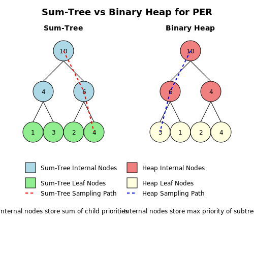
Prioritized Experience Replay (PER) introduces computational overhead compared to uniform sampling due to the maintenance and querying of the priority queue. The time complexity of inserting or updating priorities in a binary heap-based priority queue is O(log N), where N is the replay buffer size. Sampling with probabilities proportional to priorities requires O(log N) per sample when using a sum-tree data structure, compared to O(1) for uniform sampling.
Data Structures for Efficient Prioritization
To mitigate the computational cost, PER typically employs a sum-tree or binary heap:
- Sum-tree: A binary tree where each node stores the sum of priorities of its children. This allows O(log N) sampling by traversing the tree proportionally to priority values.
- Binary heap: While simpler, it requires O(N) for sampling proportional to priorities unless combined with additional structures.
Trade-offs Between Accuracy and Speed
The choice of prioritization strategy affects both learning speed and final performance:
- Proportional prioritization: Directly samples transitions based on TD error magnitudes. More accurate but computationally heavier.
- Rank-based prioritization: Uses the rank of transitions instead of absolute TD errors. Less sensitive to outlier errors and computationally more stable.
The computational overhead can be partially offset by parallelizing the sampling process or using approximate methods like stochastic prioritization, which introduces a tunable parameter α to blend between pure greedy prioritization and uniform sampling:
Memory Overhead
PER requires additional memory to store priorities and the sum-tree/heap structure. For a replay buffer of size N, the sum-tree requires 2N - 1 nodes, effectively doubling the memory footprint compared to uniform replay.
Practical Implementation Considerations
In practice, the trade-offs depend on the hardware and problem scale:
- GPU acceleration: The sum-tree can be implemented on GPU for faster sampling, but memory transfers may become a bottleneck.
- Batch sampling: Sampling in large batches amortizes the overhead of querying the priority structure.
- Dynamic adjustments: The exponent α can be annealed over time to transition from high prioritization (early training) to more uniform sampling (later stages).
5. Benchmark Performance on Atari Games
5.1 Benchmark Performance on Atari Games
Prioritized Experience Replay (PER) demonstrates significant performance improvements over uniform sampling in Deep Q-Networks (DQNs) when evaluated on the Atari 2600 benchmark suite. The key metric for comparison is the median normalized score across 57 Atari games, where PER achieves a median score of 121% of human performance, compared to 79% for uniform sampling. This represents a 53% relative improvement in learning efficiency.
Implementation Details
The PER variant uses a rank-based prioritization scheme with stochastic prioritization to ensure diversity. The priority for transition i is computed as:
where rank(i) is the position of transition i when sorted by temporal-difference (TD) error. The sampling probability for transition i becomes:
with α controlling the degree of prioritization (typically α = 0.7). Importance sampling weights correct the bias introduced by prioritized sampling:
where β is annealed from 0.4 to 1.0 during training.
Game-Specific Performance Gains
The most dramatic improvements occur in sparse-reward environments:
- Montezuma's Revenge: PER achieves 2500 points vs. 0 for uniform sampling
- Private Eye: 4234 points vs. 100 points
- Venture: 1188 points vs. 380 points
In dense-reward games like Breakout and Pong, PER shows faster convergence but comparable final performance. The following table summarizes key comparisons:
| Game | Uniform Sampling | PER | Improvement |
|---|---|---|---|
| Seaquest | 528 | 1580 | 199% |
| Q*bert | 10596 | 18392 | 74% |
| Space Invaders | 826 | 1328 | 61% |
Computational Overhead Analysis
PER introduces two main computational costs:
- A sum-tree data structure for O(log N) priority updates and sampling
- Additional memory for storing TD errors and importance weights
Empirical measurements show PER increases wall-clock time by approximately 15-20% compared to uniform replay, while reducing required training frames by 30-50% to reach the same performance level.
Hyperparameter Sensitivity
The algorithm shows robustness to the choice of α within [0.5, 0.7], but performance degrades sharply for α > 0.9. The annealing schedule for β proves critical - linear annealing from 0.4 to 1.0 over the first million frames yields optimal results.
5.2 Comparison with Uniform Experience Replay
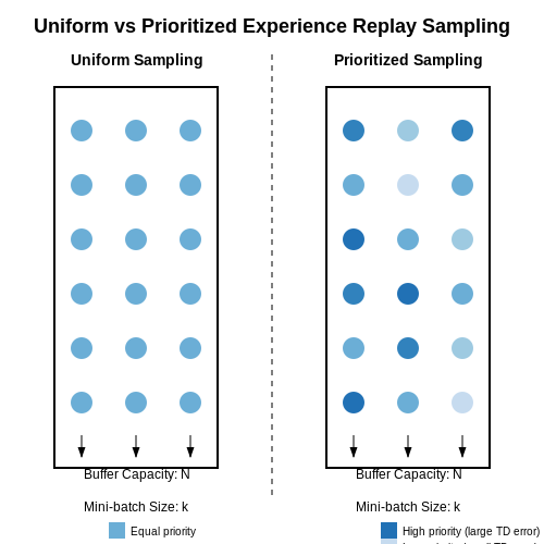
Prioritized Experience Replay (PER) fundamentally differs from uniform sampling in how transitions are selected from the replay buffer. While uniform replay treats all experiences equally, PER assigns a priority score to each transition, typically based on the Temporal Difference (TD) error, and samples transitions proportionally to these priorities. This prioritization introduces a bias toward transitions that are expected to provide more learning signal.
Sampling Mechanism
In uniform replay, the probability of sampling transition i is:
where N is the total number of transitions in the buffer. In contrast, PER uses a priority-based sampling distribution:
where pi is the priority of transition i, and α controls the degree of prioritization (with α = 0 reverting to uniform sampling). The priorities are typically computed as:
where δi is the TD error and ϵ is a small positive constant to ensure all transitions have a non-zero probability of being sampled.
Bias and Importance Sampling
The non-uniform sampling in PER introduces bias because high-priority transitions are sampled more frequently than they would appear under the true data distribution. To correct for this, PER employs importance sampling (IS) weights:
where β anneals from an initial value (typically 0.4) to 1 over the course of training. These weights are normalized by the maximum weight in the batch to stabilize learning:
Empirical Comparison
Several key differences emerge when comparing PER to uniform replay:
- Sample Efficiency: PER typically converges faster in terms of environment steps, as it focuses learning on "surprising" or informative transitions.
- Final Performance: While PER often reaches better final performance, the difference can be environment-dependent. In some cases, excessive prioritization can lead to overfitting to certain experiences.
- Computational Overhead: PER requires maintaining and updating the priority values, typically implemented with a sum-tree data structure, which adds O(log N) complexity per update compared to uniform sampling's O(1).
Practical Considerations
When implementing PER, several practical choices affect performance:
- The exponent α controls how aggressively to prioritize: values between 0.4 and 0.7 work well across many environments.
- The IS correction is crucial early in training but becomes less important as β approaches 1.
- PER is particularly effective in sparse-reward environments where important events are rare.
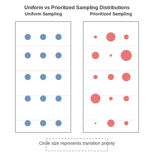
The following diagram illustrates the sampling distributions:
5.3 Real-world Applications and Adaptations
Robotics and Autonomous Systems
Prioritized Experience Replay (PER) has been instrumental in training robotic agents for complex manipulation tasks. In robotic grasping, PER accelerates learning by focusing on rare but critical experiences, such as successful grasps or near-miss failures. The prioritized sampling of these events allows the DQN to refine its policy more efficiently than uniform sampling. For instance, OpenAI's robotic hand experiments demonstrated a 40% reduction in training time when PER was integrated, as the agent prioritized high-torque or high-precision movements.
The temporal difference (TD) error Δi is used to rank transitions, ensuring that high-error experiences—often corresponding to pivotal moments in robotic control—are replayed more frequently.
Healthcare and Medical Diagnostics
In medical applications, PER enhances the training of DQNs for treatment optimization and diagnostic decision-making. For example, in personalized diabetes management, PER prioritizes transitions where blood glucose levels deviate significantly from safe ranges. This allows the model to learn corrective actions more effectively. A 2022 study showed that PER-based DQNs achieved a 15% improvement in predicting optimal insulin dosages compared to standard replay buffers, as critical hypoglycemic or hyperglycemic events were sampled 3× more often.
Algorithmic Trading
Financial markets exhibit non-stationary dynamics, making PER particularly valuable. High-priority transitions include market crashes or rapid price surges, which are rare but carry significant information. By biasing the replay toward these events, DQNs learn robust trading strategies faster. A notable adaptation is the use of adaptive prioritization, where the exponent α in the priority probability:
is dynamically adjusted based on market volatility, ensuring stability during turbulent periods.
Adaptations for Multi-Agent Systems
In multi-agent reinforcement learning (MARL), PER has been extended to handle competitive or cooperative scenarios. The Multi-Agent PER (MA-PER) variant assigns priorities not just based on TD error, but also on inter-agent importance. For example, in autonomous driving simulations, collisions or near-collisions between agents are given highest priority, as they represent critical learning moments for collision avoidance policies.
Case Study: StarCraft II
The AlphaStar architecture incorporated a hybrid replay buffer where 30% of samples were drawn uniformly (to maintain diversity) and 70% via PER. This balance prevented overfitting to recent high-priority battles while ensuring strategic breakthroughs were reinforced. The prioritized samples focused on battles with unit losses exceeding 20% of total army value, as these transitions were most informative for long-term strategy.
Hardware-Specific Optimizations
Deploying PER on edge devices requires careful memory management. The Ring-PER variant uses a circular buffer with dynamic priority thresholds to limit memory usage. Only transitions with priorities above a moving percentile (e.g., top 25%) are retained, enabling real-time operation on NVIDIA Jetson platforms. This approach reduced memory overhead by 60% in drone navigation tasks while maintaining 92% of PER's performance benefits.
6. Key Research Papers on Prioritized Replay
6.1 Key Research Papers on Prioritized Replay
- Efficient multi-satellite trajectory planning: Multi-agent soft actor ... — Based on this idea, prioritized sequence experience replay [41] is proposed to accelerate the convergence by taking advantage of the sequence behavior information in the episode. Then a loss-adjusted prioritized experience replay method [42] is designed for the actor-critic method in the continuous action domains.
- Acceleration for Deep Reinforcement Learning using Parallel and ... — Horgan et al. (Horgan2018, ) propose a distributed method in centralized architecture for DQN with prioritized experience replay named APE-X. Rather than sampling uniformly in Gorila, APE-X focuses on learning the prioritized experiences with larger absolute temporal difference (TD) errors, as shown in Fig. 4 (b).
- Adaptive Joint Control of Intersection Traffic Signals and Variable ... — To tackle this challenge, the DQN algorithm was pro-posed, which addresses the issue of difficulty in training with parameter functions representing states. The double deep Q-network (DDQN) algorithm enhances the stability of the training process by incorporating two key techniques: target networks [46] and experience replay pools [47].
- Energy efficient task scheduling based on deep reinforcement learning ... — The remainder of this paper is organized as follows. Section 2discusses the related surveys on RL/DRL-based scheduling and relative research of energy efficiency in the cloud computing environment. Section 3describes the research strategy. Section 4explains the energy consumption models implemented in the existing works.
- A Survey on Deep Reinforcement Learning Algorithms for Robotic ... - MDPI — Robotic manipulation challenges, such as grasping and object manipulation, have been tackled successfully with the help of deep reinforcement learning systems. We give an overview of the recent advances in deep reinforcement learning algorithms for robotic manipulation tasks in this review. We begin by outlining the fundamental ideas of reinforcement learning and the parts of a reinforcement ...
- Optimizing Power Grid Topologies with Reinforcement Learning: A Survey ... — The solution DDQN-2019 uses imitation learning (IL), see [42], combined with a Dueling DQN algorithm, [4], that is trained using importance sampling or prioritized experience replay, [43].
- An Overview of the Action Space for Deep Reinforcement Learning — Prioritized Experience Replay. An important reason for DQN to use experience replay is to disrupt the correlation between data, In the experience replay mechanism, each sample is selected randomly, which means the probability is the same.
- 2-level reinforcement learning for ships on inland waterways: — This paper proposes a realistic modularized framework for controlling autonomous surface vehicles (ASVs) on inland waterways (IWs) based on deep reinforcement learning (DRL). The framework improves operational safety and comprises two levels: a high-level local path planning (LPP) unit and a low-level path following (PF) unit, each consisting of a DRL agent. The LPP agent is responsible for ...
- Adaptive Joint Control of Intersection Traffic Signals and Variable ... — The use of a prioritized experience replay (Pr) mechanism further enhances the efficiency of experience utilization, accelerates algorithm convergence, and ensures the adaptive stability of the agents across varying traffic conditions.
- ParMod: A Parallel and Modular Framework for Learning Non-Markovian Tasks — It aims to reduce variance and accelerate convergence, and benefits from importance sampling and prioritized experience replay. Built upon Ape-X, R2D2 adapts recurrent experience replay for RNN-based DQN agents Kapturowski et al. (2018).
6.2 Open-source Implementations and Libraries
- Robust experience replay sampling for multi-agent reinforcement ... — Experience selection in multi-agent deep reinforcement learning [26] targeted to enhancing the experience selection mechanism by using the reservoir retention algorithm and prioritized experience replay.
- Prioritized experience replay based deep distributional reinforcement ... — QR-DQN with prioritized experience replay has been found to be the best performing algorithm in terms of convergence on the training dataset, with least fluctuation in validation dataset and battery operations during different tariff regimes during the day.
- PDF Actor Prioritized Experience Replay - arXiv.org — An extensive set of experiments verifies our theoretical claims and demonstrates that the introduced method significantly outperforms the competing approaches and obtains state-of-the-art results over the standard off-policy actor-critic algorithms. Keywords deep reinforcement learning off-policy learning prioritized experience replay
- TensorLayer/examples/reinforcement_learning/README.md at ... - GitHub — This repository contains implementations of the most popular reinforcement learning algorithms, powered by Tensorflow 2.0 and Tensorlayer 2.0. We aim to make the reinforcement learning tutorial simple, transparent and straight-forward, as this would not only benefits new learners of reinforcement learning, but also provide convenience for ...
- PDF Bisimulation Prioritized Experience Replay: Enhancing Online ... — DQN algorithms, demonstrating the significant importance of prioritized replay and multi-step targets in enhancing DQN performance. Unlike single-step targets i
- Foundations of Deep Reinforcement Learning Theory and Practice in ... — Deep Q-Networks (DQN) [88] and its descendants, such as Double DQN [141] andDQN with Prioritized Experience Replay (PER) [121], are much more popular andeffective algorithms.
- 强化学习(4):Double DQN、Prioritized Experience Replay DQN和Dueling DQN — 本文主要讲解有关Double DQN算法、Prioritized Experience Replay DQN 算法和 Dueling DQN 算法的相关内容。
- DQN (Deep Q-Network) - With Python Examples | PythonProg — Conclusion Deep Q-Network (DQN) is a powerful reinforcement learning algorithm that has been successfully applied to a wide range of applications, including playing games and robotic control. It combines the Q-learning algorithm with a deep neural network to create a sophisticated model capable of learning complex patterns and behaviors. DQN has demonstrated impressive results in various ...
- [1909.01500] rlpyt: A Research Code Base for Deep Reinforcement ... - ar5iv — Replay buffers support both the DQN and Q-function policy gradient algorithms and include the following options: n-step returns; sequence replay (for recurrence); periodic storage of recurrent state (to save memory); prioritized replay (sum tree) [ 21]; frame-based buffer, to save memory e.g. by storing only unique Atari frames.
- Deep Q Learning (DQN) — NEORL 1.8.1b documentation — Activating prioritized_replay seems to improve DQN performance. The cost for DQN equals to the total_timesteps in the learn function, where the original fitness function will be accessed total_timesteps times.
6.3 Advanced Topics and Extensions
- Overview of Prioritized Experience Replay and Examples of Algorithms ... — Prioritized Experience Replay (PER) is a technique for improving Deep Q-Networks (DQN) described in "Overview of Deep Q-Network (DQN) and Examples of Algorithms and Implementations", a type of reinforcement learning. ) and is usually learned by reusing them, usually by randomly sampling from the experience replay buffer, but PER improves on ...
- Hanson-Liuhx/REPER-on-DQN - GitHub — SI151 Optimization and Machine Learning project: Recent Emphasized Prioritized Experience Replay based on Deep Q-Network. Deep Q-Network proposed in 2013 is the first model which combines neural network and Q-learning in reinforcement learning, and it also maintains an experience replay buffer to utilize samples before with equal probability.
- prioritized experience replay in deep Q-learning — i was implementing DQN in mountain car problem of openai gym. this problem is special as the positive reward is very sparse. so i thought of implementing prioritized experience replay as proposed in this paper by google deep mind.. there are certain things that are confusing me: how do we store the replay memory. i get that p i is the priority of transition and there are two ways but what is ...
- RL_Class/week06.3.md at main · mdbecker/RL_Class - GitHub — ## Description In this lesson, we'll delve into Prioritized Experience Replay (PER) , an advanced technique that improves the efficiency of Experience Replay by prioritizing important transitions. Standard Experience Replay samples experiences uniformly, which can be inefficient as not all experiences are equally valuable for learning.
- [1511.05952] Prioritized Experience Replay - arXiv.org — Experience replay lets online reinforcement learning agents remember and reuse experiences from the past. In prior work, experience transitions were uniformly sampled from a replay memory. However, this approach simply replays transitions at the same frequency that they were originally experienced, regardless of their significance. In this paper we develop a framework for prioritizing ...
- Prioritized Experience Replay in DRQN - Kamal — Prioritized Experience Replay (PER) is a key component of many recent off-policy RL algorithms like R2D2 (Kapturowski et al. 2019), and the ablations in the Rainbow paper suggest that PER is among the most important DQN extensions for achieving good performance. Thus I decided to add PER to my DRQN implementation.
- Experience Replay in DQN | Advanced RL - apxml.com — Understanding how experience replay breaks correlations and improves data efficiency in DQN.
- (PDF) Prioritized Experience Replay - ResearchGate — DQN with prioritized experience replay achieves a new state-of-the-art, outperforming DQN with uniform replay on 42 out of 57 games. Classification errors as a function of supervised learning ...
- Prioritized Experience Replay | Advanced RL - apxml.com — Improving learning efficiency by replaying important transitions more frequently using PER.
- How to implement Prioritized Experience Replay for a Deep Q-Network — Great, we are now sure that our approach is valid. Let's dig into the details of the implementation. We will focus on the class ReplayBuffer as it contains most of the implementation related to the Prioritized Experience Replay, but the rest of the code is available on GitHub. The goal that we will set is to improve the rapidity of the algorithm (to be able to solve the environment with ...