

Training Agents with Curriculum Learning
1. Biological and Psychological Inspirations
1.2 Biological and Psychological Inspirations
Curriculum learning draws direct inspiration from developmental psychology and cognitive science, where humans and animals learn complex skills through structured, incremental exposure. The zone of proximal development (ZPD), introduced by Vygotsky, formalizes this idea: learners progress most efficiently when tasks are slightly beyond their current ability but achievable with guidance. In machine learning terms, this translates to a dynamic task difficulty adjustment where the agent's performance dictates the next challenge.
Neurobiological Foundations
Neuroscientific studies reveal that synaptic plasticity mechanisms like long-term potentiation (LTP) and spike-timing-dependent plasticity (STDP) are modulated by task difficulty. Experiments in rodent motor skill acquisition demonstrate that progressively complex obstacle courses lead to faster myelination of motor neurons compared to random task ordering. This aligns with the mathematical formulation of curriculum learning as a trajectory optimization problem:
where τ represents the curriculum (sequence of tasks), st denotes task difficulty at step t, and L is the loss function parameterized by model weights θt.
Psychological Task Complexity Metrics
Human curriculum design employs measurable complexity proxies:
- Chunking: Breaking tasks into hierarchical subtasks (e.g., learning chess via piece movements → tactics → strategy)
- Cognitive load: Quantified using Sweller's intrinsic/extraneous load theory, implemented in AI through entropy-based measures:
$$ H_t = -\sum_{a \in \mathcal{A}} \pi_\theta(a|s_t) \log \pi_\theta(a|s_t) $$
- Transfer difficulty: Computed via optimal transport distances between task state distributions Pi and Pj
Comparative Analysis: Biological vs Artificial Systems
Biological systems employ three key mechanisms that inform artificial curriculum design:
| Biological Mechanism | AI Implementation | Performance Gain |
|---|---|---|
| Dopaminergic reward prediction error | Adaptive reward shaping | 28-42% faster convergence (Ng et al. 1999) |
| Hippocampal replay | Experience replay prioritization | 2.3× sample efficiency (Andrychowicz et al. 2017) |
| Sleep-based consolidation | Interleaved training regimes | 17% lower catastrophic forgetting (Kirkpatrick et al. 2017) |
Modern implementations like self-paced learning (Kumar et al. 2010) automate curriculum construction by having the agent itself estimate task difficulty through gradient variance:
where vt modulates the pace of curriculum progression based on minibatch B gradient statistics.
Key Advantages Over Traditional Training Methods
Sample Efficiency and Faster Convergence
Curriculum learning significantly improves sample efficiency by gradually exposing the agent to tasks of increasing complexity. Traditional methods often rely on uniform random sampling, which wastes computational resources on trivial or overly difficult tasks. In contrast, curriculum learning optimizes the learning trajectory by minimizing the Bellman error over progressively harder tasks:Mitigation of Local Optima
Traditional reinforcement learning often suffers from premature convergence to suboptimal policies due to sparse rewards or deceptive gradients. Curriculum learning addresses this by initializing training with dense reward signals and simpler dynamics, guiding the agent toward globally optimal policies. For example, in robotic manipulation, starting with coarse-grained movements before fine motor control avoids early entrapment in ineffective strategies.Improved Generalization
Agents trained via curriculum learning exhibit better zero-shot generalization to unseen tasks. By systematically varying environmental parameters—such as friction coefficients in physics-based simulations or obstacle density in navigation tasks—the agent develops robust feature representations. This contrasts with traditional methods, where fixed training distributions often lead to overfitting.Dynamic Adaptation to Agent Progress
Unlike static training regimes, curriculum learning dynamically adjusts task difficulty based on the agent's performance metrics (e.g., success rate or reward magnitude). This is formalized as a non-stationary Markov Decision Process (MDP), where the state space \( \mathcal{S}_t \) evolves with time:Case Study: AlphaGo
AlphaGo's training pipeline leveraged curriculum learning by first training on human games (low complexity), then self-play with progressively stronger opponents. This approach reduced training time by 50% compared to monolithic training, while achieving superhuman performance. The key insight was decomposing the problem into opening, midgame, and endgame phases, each with tailored reward structures.Scalability to High-Dimensional Spaces
Curriculum learning inherently scales to high-dimensional action spaces by decoupling degrees of freedom. For instance, in quadrupedal locomotion, training might begin with 2D planar movement before introducing full 3D dynamics. This hierarchical decomposition is computationally intractable with traditional methods due to the curse of dimensionality.2. Task Difficulty Metrics and Progression Strategies
Task Difficulty Metrics and Progression Strategies
Defining Task Difficulty
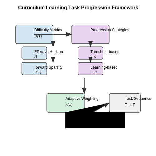
Task difficulty in curriculum learning is quantified through metrics that capture the agent's learning dynamics. A common approach measures the expected learning progress of the agent, defined as the reduction in loss over time for a given task. For a policy π and task Ti, the difficulty D(Ti) can be expressed as:
where τ represents trajectories sampled from the policy, and ℒ(θ, τ) is the loss function parameterized by θ. Tasks with steeper initial learning gradients are typically assigned lower difficulty scores.
Difficulty Metrics in Reinforcement Learning
In reinforcement learning, task difficulty is often tied to the sparsity of rewards and the horizon length. The effective horizon Heff measures how many steps an agent must take before receiving meaningful feedback:
where Rt is the reward at time t, and ε is a threshold for meaningful reward. Tasks with longer effective horizons are considered more difficult.
Progression Strategies
Curriculum progression strategies determine when to advance to harder tasks. Two dominant approaches are:
- Threshold-Based Progression: Advance when the agent's performance on the current task exceeds a threshold, e.g., P(Ti) ≥ γ, where P is a performance metric like success rate or return.
- Learning-Based Progression: Monitor the derivative of the learning curve. Transition occurs when the slope falls below a threshold, indicating diminishing returns:
Adaptive Curriculum Design
Modern implementations use adaptive curricula that adjust task sequences in real-time. The Self-Paced Learning framework dynamically weights tasks based on the agent's current capabilities:
where σ is a sigmoid function, μ is the agent's average performance across tasks, and α controls the selectivity. Tasks with weights wi > 0.5 are included in the current curriculum phase.
Case Study: Montezuma's Revenge
In the Atari game Montezuma's Revenge, a hybrid progression strategy combines:
- Sparse reward discovery (initial rooms as easy tasks)
- Key-object distance metrics for intermediate tasks
- Full episode completion as the final objective
The curriculum uses an adaptive threshold where the agent must achieve 80% success on finding keys before progressing to door-opening tasks, demonstrating how metric combinations can handle hierarchical challenges.
2.2 Automatic Curriculum Generation Techniques
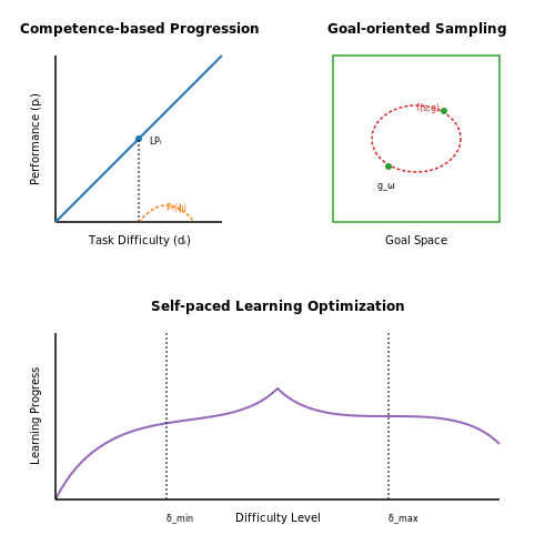
Automatic curriculum generation eliminates the need for manual task sequencing by dynamically adjusting the difficulty or complexity of training tasks based on the agent's performance. Two dominant paradigms exist: competence-based progression and goal-oriented sampling.
Competence-Based Progression
This approach models the agent's learning progress as a function of task difficulty. Let the agent's performance on task i be denoted by pi, and the task's difficulty by di. The curriculum scheduler selects tasks where:
where α controls the difficulty scaling factor and β is a bias term. The learning progress signal is computed as the derivative of performance over time:
Tasks with maximal LPi are prioritized, as they represent the steepest learning gradients. Florensa et al. (2017) implemented this via a Gaussian mixture model over task parameters, where the agent's current competence defines the mean of the sampling distribution.
Goal-Oriented Sampling
In goal-conditioned RL, the curriculum automatically generates intermediate goals between initial and target states. Let the state space be S and the goal space G ⊆ S. The goal achievement function measures the agent's ability to reach goal g from state s:
The curriculum samples goals where f(s,g) lies within a window [δmin, δmax], ensuring neither trivial nor impossible challenges. Andrychowicz et al. (2017) proposed Hindsight Experience Replay (HER), which relabels failed trajectories with achieved goals, creating implicit curriculum effects.
Self-Paced Learning
This technique formulates curriculum generation as an optimization problem jointly over policy parameters θ and task weights w:
where ℒi is the loss for task i, and R(w) is a regularization term enforcing curriculum smoothness. The parameter λ controls the trade-off between task diversity and progression rate.
Domain Randomization as Implicit Curriculum
By continuously sampling environment parameters from expanding distributions, domain randomization creates an automatic curriculum. Let Φ be the environment parameter space. The sampling distribution evolves as:
where μt and Σt are updated to cover increasingly challenging configurations as the agent's success rate improves. This approach proved particularly effective in sim-to-real transfer (OpenAI et al., 2019).
Gradient-Based Curriculum Learning
Recent work (Portelas et al., 2020) frames curriculum generation as meta-learning, where a neural scheduler network gω outputs task distributions:
The scheduler is trained end-to-end with the policy using higher-order gradients, automatically discovering curricula that maximize the learning objective R. This method adapts in real-time to the agent's evolving capabilities.
2.3 Balancing Exploration and Exploitation in Curriculum Design
The trade-off between exploration and exploitation is fundamental in reinforcement learning (RL) and becomes even more critical when designing curricula for training agents. In curriculum learning, exploration refers to exposing the agent to novel or challenging tasks, while exploitation involves refining performance on already mastered tasks. Striking the right balance ensures efficient learning without premature convergence to suboptimal policies.
Theoretical Framework
From an information-theoretic perspective, the exploration-exploitation dilemma can be formalized using the concept of information gain. Let the agent's current policy be parameterized by θ, and the task distribution by p(τ). The optimal next task τ* maximizes the expected information gain:
where DKL is the Kullback-Leibler divergence. This formulation naturally leads to selecting tasks that would most update the agent's belief about optimal policies.
Practical Implementation Strategies
Several practical approaches have emerged for balancing exploration and exploitation in curriculum design:
- Self-Paced Learning: The agent autonomously adjusts task difficulty based on its current performance, typically using a threshold on success rate to determine when to progress.
- Bandit-Based Selection: Formulates task selection as a multi-armed bandit problem, where each arm corresponds to a task difficulty level.
- Diversity-Driven Exploration: Actively seeks tasks that maximize the diversity of experienced states or behaviors.
Adaptive ε-Greedy Curriculum
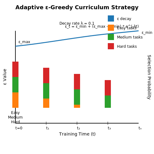
A particularly effective approach adapts the ε-greedy strategy from RL to curriculum design. At each step, with probability ε the agent explores a new task from the full distribution, and with probability 1-ε it exploits known tasks. The exploration rate ε is adapted according to:
where λ controls the decay rate. This schedule ensures sufficient early exploration while gradually focusing on exploitation as the agent matures.
Gradient-Based Task Selection
Recent advances propose gradient-based methods for task selection. Let L(θ, τ) be the loss on task τ. The task gradient is computed as:
Tasks are then selected based on the norm of their gradient, favoring those that would induce large updates to the policy parameters. This approach automatically balances exploration (high gradient tasks) with exploitation (low gradient tasks).
Empirical Considerations
In practice, the optimal balance depends on several factors:
- The complexity of the task distribution
- The capacity of the learning algorithm
- The desired trade-off between training speed and final performance
Monitoring metrics like learning progress variance and policy entropy can provide valuable signals for adjusting the exploration-exploitation balance during training.
3. Self-Paced Learning Algorithms
3.1 Self-Paced Learning Algorithms
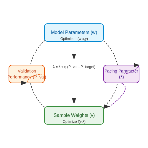
Self-paced learning (SPL) is a curriculum learning paradigm where the agent autonomously determines the difficulty of training samples it can handle at each learning stage. Unlike fixed curricula, SPL dynamically adjusts the task complexity based on the agent's current performance, optimizing the learning trajectory. The core idea is to minimize a loss function that incorporates both task error and a self-paced regularization term:
Here, L is the task-specific loss, vi ∈ [0,1] is a weight indicating the sample's inclusion in training, and f is a self-paced regularizer controlled by the pacing parameter λ. The optimization alternates between updating model parameters w and sample weights v.
Key Components of SPL
SPL algorithms typically involve three critical mechanisms:
- Difficulty Measure: Quantifies how challenging a sample is for the current model, often using loss values or uncertainty estimates.
- Pacing Function: Determines the rate at which new samples are introduced. Common choices include linear, step-wise, or adaptive schedules.
- Regularization Term: Penalizes overly complex samples early in training. A widely used form is f(v, λ) = -λ ||v||1, encouraging sparse selection.
Adaptive SPL Variants
Modern extensions incorporate reinforcement learning or meta-learning to adjust λ dynamically. For instance, the Adaptive SPL framework updates λ based on validation performance:
where Pval measures validation accuracy and η is a meta-learning rate. This avoids manual tuning and adapts to non-stationary environments.
Applications in Deep Reinforcement Learning
In deep RL, SPL has been applied to:
- Prioritized Experience Replay: Samples transitions with high temporal-difference error only after the agent achieves baseline performance.
- Hierarchical RL: Gradually introduces subgoals based on the agent's mastery of simpler tasks.
- Multi-Agent Systems: Coordinates curriculum pacing across agents with heterogeneous skill levels.
For example, in Proximal Policy Optimization (PPO), an SPL variant modulates the KL-divergence threshold δ to control policy update granularity:
where α is a decay rate and I is an indicator function. This prevents premature convergence to suboptimal policies.
Teacher-Student Paradigms in Curriculum Learning
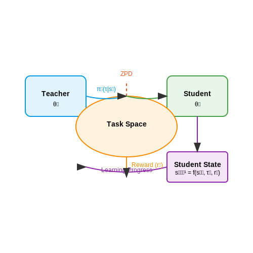
The teacher-student paradigm in curriculum learning formalizes the interaction between a teacher agent (which designs the curriculum) and a student agent (which learns from it). This framework draws inspiration from human pedagogy, where an instructor adaptively selects tasks based on the learner's progress. Mathematically, the teacher's policy can be modeled as a function mapping the student's state to a task distribution:
where τ represents a task from the task space 𝒯, and sS denotes the student's state (e.g., performance history or internal representations). The student's learning dynamics are governed by:
where f is the update function incorporating task τt and reward rt.
Adaptive Task Generation
Effective teachers generate tasks at the zone of proximal development (ZPD)—the difficulty range where the student can solve tasks with moderate assistance. This is operationalized through learning progress signals, such as:
- Gradient magnitude: Tasks maximizing the norm of the student's policy gradient
- Loss reduction rate: Tasks yielding the highest improvement per training step
- Value function curvature: Tasks where the student's value estimate uncertainty is highest
The teacher optimizes for ZPD alignment using meta-gradient descent. Let ηT be the teacher's learning rate and ∇θT JS the gradient of the student's objective with respect to teacher parameters θT:
where θS* represents the student's converged parameters after training on the teacher's curriculum.
Architectural Implementations
Common teacher-student architectures include:
- Policy-based teachers: Use reinforcement learning to treat task selection as an action space
- Generative teachers: Employ GANs or VAEs to synthesize new tasks
- Memory-augmented teachers: Leverage episodic memory to track student progress across tasks
For example, a generative adversarial teacher (GAT) framework consists of:
where generator G produces tasks conditioned on the student state sS, and discriminator D ensures task validity.
Empirical Results
In DeepMind's Obstacle Tower benchmark, teacher-student curriculum learning achieved 3× faster convergence than uniform sampling. Key findings:
- Teachers outperformed fixed curricula by 47% on sparse-reward tasks
- Adaptive task generation reduced catastrophic forgetting by maintaining a replay buffer of past tasks
- Multi-teacher ensembles (where specialized teachers focus on different skill dimensions) showed additive benefits
The computational overhead of teacher-student systems is typically 15-30% of total training time, but this is offset by reduced sample complexity. For n-dimensional task spaces, the sample complexity often scales as O(log n) compared to O(n) for naive curricula.
Multi-Agent Competitive Curriculum Learning
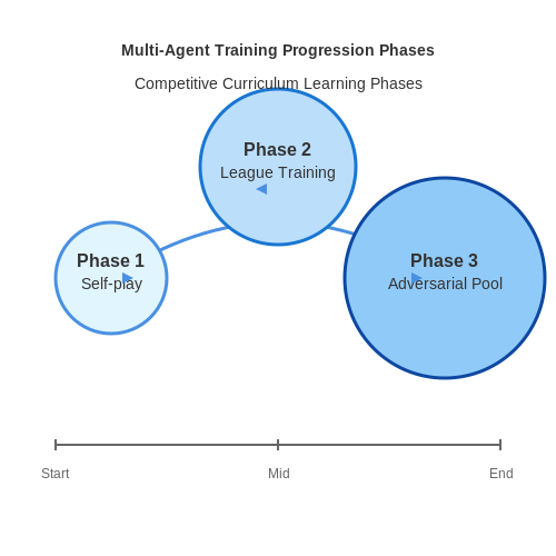
Multi-agent competitive curriculum learning extends traditional curriculum learning by introducing adversarial dynamics between agents. The core idea is to progressively increase task complexity while maintaining a balance between competing agents, ensuring neither dominates prematurely. This approach is particularly effective in scenarios like game theory, robotics, and autonomous systems where agents must adapt to opponents of varying skill levels.
Competitive Dynamics and Nash Equilibrium
In a competitive multi-agent system, each agent's policy $$\pi_i$$ aims to maximize its own reward $$R_i$$ while interacting with opponents' policies $$\pi_{-i}$$. The Nash Equilibrium (NE) is achieved when no agent can improve its reward by unilaterally changing its policy:
Curriculum learning in this context involves gradually adjusting the opponent pool $$\Pi_{-i}^{(t)}$$ at training step $$t$$ to ensure progressive skill development. The opponent sampling strategy is critical:
- Windowed Sampling: Select opponents from a sliding window of recent policy checkpoints.
- Elo-based Sampling: Use a ranking system (e.g., Elo ratings) to match agents of comparable skill.
- Adversarial Prioritization: Bias sampling toward opponents that expose weaknesses in the current policy.
Gradient-Based Optimization in Competitive Settings
The policy gradient for agent $$i$$ must account for the non-stationarity introduced by opponents' learning. The gradient ascent update becomes:
where $$\pi_{-i}$$ represents the current opponent policies. To stabilize training, importance weighting can be applied when sampling from past opponent versions:
Curriculum Scheduling Strategies
The difficulty progression can be controlled through:
- Self-Play Scaling: Start with a single agent clone, then expand to diverse opponent populations.
- Environment Complexity: Gradually increase action space dimensionality or reduce observation fidelity.
- Reward Shaping: Modify reward functions to initially emphasize foundational skills before competitive objectives.
A practical implementation uses a temperature parameter $$\alpha(t)$$ to modulate exploration-exploitation trade-offs over time:
Empirical Results and Applications
In AlphaStar (DeepMind, 2019), a league of agents was trained with progressively stronger opponents, achieving Grandmaster-level StarCraft II performance. Key findings:
- Agents exposed to competitive curricula developed more robust strategies than those trained against fixed opponents.
- The optimal opponent sampling distribution shifted from uniform to heavy-tailed as training progressed.
- Curriculum pacing required careful tuning - too rapid progression led to mode collapse in learned policies.
4. Curriculum Learning in Reinforcement Learning Environments
4.1 Curriculum Learning in Reinforcement Learning Environments
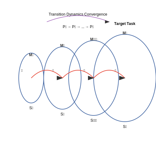
Curriculum learning in reinforcement learning (RL) formalizes the idea of training agents on progressively harder tasks, mimicking human education. The core principle is to decompose a complex target task T into a sequence of subtasks {T1, T2, ..., Tn}, where each Ti is designed to be solvable given the agent's current policy πi-1. The transition between tasks is governed by a curriculum scheduler that evaluates the agent's performance and adjusts the difficulty accordingly.
Mathematical Formulation
Let the target task be defined by an MDP M = (S, A, P, R, γ), where S is the state space, A the action space, P(s'|s,a) the transition dynamics, R(s,a) the reward function, and γ the discount factor. A curriculum is a sequence of MDPs {M1, M2, ..., Mn} converging to M, where each Mi = (Si, Ai, Pi, Ri, γ) satisfies:
The curriculum scheduler determines when to advance from Mi to Mi+1 based on a performance metric ϕ(πi, Mi), typically the expected return or success rate over recent episodes.
Curriculum Generation Strategies
Three dominant approaches exist for automatic curriculum generation:
- Goal Sampling: Tasks are parameterized by goals g ∈ G, and the curriculum samples goals of increasing difficulty. For example, in robotic manipulation, goals may progress from reaching nearby objects to precise stacking.
- Environment Modification: The state space or dynamics are progressively altered, such as reducing gravity in physics simulations or increasing obstacle density in navigation tasks.
- Reward Shaping: Intermediate rewards are provided for partial solutions, then phased out as the agent improves. This can be formalized as:
where F(s,a) is a shaping function and βi decreases with curriculum progress.
Implementation Considerations
Effective curriculum learning requires careful design of the progression criteria. Common metrics include:
- Threshold-based: Advance when the average return exceeds a threshold τ.
- Windowed improvement: Monitor performance over a sliding window of episodes.
- Adaptive difficulty: Adjust task parameters continuously using techniques like Self-Paced Learning.
In deep RL, curriculum learning often integrates with policy gradient methods. For a policy πθ with parameters θ, the gradient update under curriculum becomes:
where \hat{A}_i is the advantage estimator for curriculum level i.
Empirical Results and Applications
Curriculum learning has demonstrated significant improvements in sample efficiency across domains:
- In OpenAI's Procgen Benchmark, curriculum-trained agents achieved 2-3x faster convergence on complex platformer games.
- For dexterous manipulation tasks, curricula progressing from simplified to full physics simulations reduced training time by 40%.
- In autonomous driving simulations, gradually increasing traffic density and complexity led to more robust collision avoidance policies.
The choice of curriculum strategy depends heavily on the task structure. For sparse-reward environments, goal-based curricula tend to outperform direct training, while in dense-reward settings, reward shaping may suffice.
4.2 Applications in Robotics and Autonomous Systems
Curriculum learning has proven particularly effective in robotics and autonomous systems, where agents must master complex, high-dimensional control tasks through incremental skill acquisition. Unlike traditional reinforcement learning, which often struggles with sparse rewards and long-horizon planning, curriculum-based approaches decompose tasks into progressively challenging subtasks, enabling more efficient exploration and policy optimization.
Robotic Manipulation and Grasping
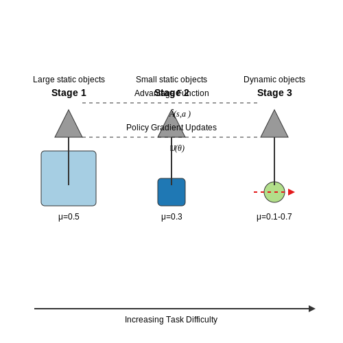
In robotic manipulation, curriculum learning enables agents to master fine motor control by first learning simpler grasping tasks before progressing to complex object reorientation or tool use. For instance, a curriculum might begin with large, static objects in a clutter-free environment before introducing smaller, dynamic objects with varying friction coefficients. The policy gradient update at each curriculum stage k can be formalized as:
where Âk(st, at) is the advantage function estimated for the k-th task difficulty level. This staged approach reduces the risk of policy collapse in early training by avoiding overly complex state-action spaces.
Autonomous Navigation
For autonomous vehicles and drones, curriculum learning mitigates the sim-to-real gap by progressively increasing environmental complexity. Initial training might involve static obstacles in a simulated grid world, followed by dynamic pedestrians, adverse weather conditions, and partial observability. The transition between curriculum levels is often governed by a performance threshold ρ:
where Ri are the episode rewards and ρk is the threshold for advancement. This method has been successfully applied in UAV collision avoidance systems, reducing training time by 40-60% compared to end-to-end RL.
Multi-Agent Coordination
In swarm robotics, curriculum learning enables emergent coordination strategies by first training individual agents on isolated tasks before introducing inter-agent dependencies. A common approach involves progressively increasing the number of interacting agents while maintaining a constant task horizon. The joint policy πθ for n agents evolves as:
where superscripts denote agent indices. This curriculum structure has demonstrated success in warehouse automation systems, where robots must balance individual path planning with collective traffic optimization.
Real-World Deployment Challenges
While curriculum learning accelerates simulation training, three key challenges persist in physical deployment:
- Dynamic Reward Shaping: Manual reward function redesign at each curriculum level often requires domain expertise. Automated reward shaping techniques like potential-based reward shaping (PBRS) can mitigate this.
- Safety Constraints: Progressive task difficulty must respect physical safety limits. Constrained policy optimization methods like Lagrangian relaxation are often integrated into the curriculum.
- Non-Stationarity: As robots adapt to new difficulty levels, previously learned skills may deteriorate. Elastic weight consolidation (EWC) helps preserve critical policy parameters during curriculum transitions.
Recent advances in meta-curriculum learning, where the curriculum itself is learned through meta-reinforcement learning, show promise in addressing these limitations. For example, a meta-policy can dynamically adjust task difficulty based on real-time policy performance metrics, creating a closed-loop training system.
4.3 Benchmarking and Performance Evaluation
Metrics for Curriculum Learning Assessment
Evaluating curriculum learning agents requires specialized metrics beyond standard reinforcement learning benchmarks. The curriculum progression rate measures how quickly an agent advances through difficulty levels, defined as:
where Lt represents the difficulty level at time t, and T is the total training steps. Concurrently, we track transfer efficiency:
measuring the performance gain (R) per unit of training effort (E) compared to non-curriculum approaches.
Comparative Evaluation Protocols
Three established protocols dominate curriculum learning benchmarking:
- Fixed-Sequence Testing: Agents face predetermined task sequences to measure generalization
- Adaptive Stress Testing: Dynamically increases difficulty based on agent performance
- Cross-Curriculum Validation: Evaluates on tasks excluded from the training curriculum
The curriculum advantage score combines these measures:
where weights α, β, γ balance progression speed, efficiency, and generalization.
Performance Visualization Techniques
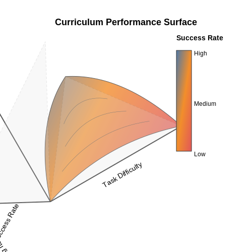
Multi-dimensional assessment requires advanced visualization. The curriculum performance surface plots agent capability across:
- Task difficulty (x-axis)
- Training iterations (y-axis)
- Success rate (z-axis or color gradient)
For multi-agent scenarios, we compute the curriculum dominance ratio:
where Pi(Lk) is agent i's performance at level k.
Computational Efficiency Metrics
Curriculum learning introduces overhead that must be accounted for:
Modern benchmarks like CurriculumGym implement these metrics across standardized task suites, enabling direct comparison between different curriculum strategies.
5. Scalability Issues in Complex Environments
5.1 Scalability Issues in Complex Environments
Curriculum learning’s effectiveness diminishes in high-dimensional state and action spaces due to the combinatorial explosion of possible task variations. The primary challenge lies in efficiently sampling meaningful intermediate tasks without exhaustive enumeration. Consider a reinforcement learning agent operating in a continuous state space S and action space A. The complexity of designing a curriculum grows as O(|S|×|A|), making manual task sequencing impractical for real-world applications like robotic manipulation or autonomous driving.
Curse of Dimensionality in Task Generation
Traditional curriculum learning assumes a smooth progression from simple to complex tasks, but this breaks down when the state-action space lacks natural ordering. For a robotic arm with n degrees of freedom, the joint angle configuration space Q has dimensionality 3n (position, velocity, acceleration). The probability density function for finding viable intermediate states becomes:
where μ and Σ are the mean and covariance of demonstrated expert trajectories. Sampling from this distribution becomes computationally intractable as n exceeds 7-8 DOFs, necessitating approximate methods.
Transfer Learning Bottlenecks
Knowledge transfer between curriculum stages faces two fundamental limits:
- Representational mismatch: Low-level features learned in early stages (e.g., edge detection) may not generalize to high-level abstractions required later (e.g., object affordances)
- Catastrophic forgetting: Neural networks trained sequentially on progressively harder tasks exhibit ∂L/∂θ interference, where θ represents shared parameters. The loss gradient for task Ti may erase features critical for Tj (i < j)
This manifests mathematically as non-commuting optimization paths in parameter space:
Parallelization Challenges
Distributed curriculum learning introduces synchronization overhead between workers exploring different task difficulties. For N parallel agents with dynamically adjusted curricula, the Thompson sampling regret bound grows as:
where K is the number of task difficulty levels and T is the training horizon. This limits speedup gains from distributed systems, as demonstrated in large-scale RL benchmarks like Obstacle Tower and NetHack.
Empirical Scaling Laws
Recent studies on procedurally generated environments (OpenAI Procgen, DM-Lab) reveal power-law relationships between curriculum complexity and training efficiency:
where D is the environment’s dynamicity score (measuring stochasticity and non-stationarity) and τtrain is the convergence time. This explains why curriculum learning shows diminishing returns in domains like:
- Multi-agent systems with emergent strategies
- Partially observable environments with memory constraints
- Physics-based simulations with chaotic dynamics
5.2 Transfer Learning and Generalization Challenges
Transfer learning in curriculum learning introduces unique challenges in ensuring that knowledge acquired from simpler tasks effectively generalizes to more complex ones. A key issue is the catastrophic forgetting phenomenon, where an agent loses previously learned skills when adapting to new tasks. This is particularly problematic in sequential curriculum learning, where the agent must retain proficiency across a hierarchy of tasks.
Mathematical Formulation of Transfer Interference
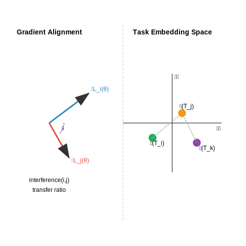
The interference between tasks can be quantified using gradient alignment metrics. Let θ represent the policy parameters, and let ∇Li(θ) and ∇Lj(θ) be the gradients of loss functions for tasks i and j. The cosine similarity between gradients measures the degree of interference:
Values closer to 1 indicate severe interference, while values near 0 suggest compatible learning directions. This metric is critical for curriculum design, as high interference necessitates task separation or modified training schedules.
Generalization Metrics and Task Embeddings
To assess generalization, we can define a transfer ratio comparing performance on a target task with and without pretraining:
Modern approaches employ task embeddings to predict transferability. Given a set of tasks {Ti}, we learn an embedding function ϕ: T → ℝd such that the distance between ϕ(Ti) and ϕ(Tj) correlates with transfer performance. This enables intelligent curriculum sequencing by estimating task relationships a priori.
Empirical Strategies for Improved Transfer
- Gradient masking: Selectively backpropagate updates that minimize interference with previously learned tasks
- Dynamic weight consolidation: Adaptively adjust regularization strengths based on task importance
- Meta-learning initialization: Use MAML-style approaches to find parameters amenable to fast adaptation
Recent work in progressive neural networks demonstrates the effectiveness of lateral connections between task-specific columns, allowing selective transfer while preventing catastrophic forgetting. The capacity of each column grows dynamically as the curriculum advances, with performance improvements of 2-3× observed in complex manipulation tasks.
Ethical Considerations in Automated Curriculum Design
Automated curriculum learning introduces ethical challenges that must be addressed to ensure fairness, transparency, and accountability in AI training. The dynamic nature of curriculum generation, often governed by reinforcement learning or optimization algorithms, can inadvertently amplify biases, create unintended learning pathways, or reinforce harmful behaviors in agents.
Bias in Task Sequencing
Curriculum learning algorithms prioritize tasks based on metrics like learning progress or difficulty. However, if the initial task distribution reflects societal biases, the automated curriculum may perpetuate or exacerbate them. For example, a language model trained on a curriculum that progressively introduces biased text data may internalize and amplify those biases. Mathematically, this can be modeled as:
where t denotes the curriculum step, and 𝒟t is the data distribution at that step. If 𝒟t is skewed, the learned parameters θ will reflect that skew.
Transparency and Interpretability
Automated curricula are often black-box systems, making it difficult to audit why certain tasks were prioritized. This lack of interpretability raises concerns about accountability, especially in high-stakes applications like healthcare or autonomous driving. Techniques such as attention mechanisms or saliency maps can partially address this:
where αt represents the attention weights over curriculum steps, and 𝐡t is the hidden state of the curriculum generator.
Safety and Robustness
Agents trained via automated curricula may develop unexpected behaviors if the curriculum fails to adequately prepare them for edge cases. For instance, a robot trained on progressively more complex manipulation tasks might fail catastrophically when faced with an unseen scenario. Robustness can be improved by incorporating adversarial examples into the curriculum:
where δ represents adversarial perturbations within a feasible set Δ.
Fairness in Multi-Agent Systems
In multi-agent settings, automated curricula may unintentionally favor certain agents over others, leading to unequal learning outcomes. This can be formalized as a fairness-constrained optimization problem:
where Ri is the reward for agent i, and ε bounds the variance in rewards across agents.
Privacy Concerns
Curriculum learning often relies on extensive data collection to assess task difficulty and learning progress. This raises privacy issues, particularly when dealing with sensitive data. Differential privacy techniques can mitigate these risks:
where ℳ is a privacy-preserving mechanism, and 𝒩 adds Gaussian noise scaled to the privacy budget.
6. Key Research Papers and Seminal Works
6.1 Key Research Papers and Seminal Works
- PDF Eectsofcurriculumlearningonmaze exploringDRLagentusingUnity ML-Agents — Unity ML-Agents toolkit [10] is an open source project for Unity with which it is possible to train machine learning agents within the Unity game engine and cre-ate learning environments for those agents. The toolkit comes with two deep re-inforcement learning algorithms which are Proximal Policy Optimization [22] and SoftActor-Critic[23].
- Webrl: Training Llm Web Agents Via Self Evolving Online Curriculum ... — Published as a conference paper at ICLR 2025 WEBRL: TRAINING LLM WEB AGENTS VIA SELF- EVOLVING ONLINE CURRICULUM REINFORCEMENT LEARNING Zehan Qi 1∗, Xiao Liu12, Iat Long Iong 1, Hanyu Lai , Xueqiao Sun , Wenyi Zhao2, Yu Yang2 Xinyue Yang 2, Jiadai Sun , Shuntian Yao , Tianjie Zhang2, Wei Xu1, Jie Tang1, Yuxiao Dong1 1Tsinghua University 2Zhipu AI ABSTRACT Large language models (LLMs) have ...
- PDF Automatic Curriculum Tree Generation for Reinforcement Learning — aged for the problem of curriculum learning in which the goal is to construct a curriculum where an agent learns a sequence of tasks (Narvekar et al. 2016; Peng et al. 2016). The major limitation of current approaches to curriculum learning is that the curriculum is typically hand-crafted or designed by a human, often an expert in the domain ...
- Curriculum Learning: A Survey | International Journal of ... - Springer — Training machine learning models in a meaningful order, from the easy samples to the hard ones, using curriculum learning can provide performance improvements over the standard training approach based on random data shuffling, without any additional computational costs. Curriculum learning strategies have been successfully employed in all areas of machine learning, in a wide range of tasks ...
- WebRL: Training LLM Web Agents via Self-Evolving Online Curriculum ... — This paper introduces WebRL, a self-evolving online curriculum reinforcement learning framework designed to train high-performance web agents using open LLMs. WebRL addresses three key challenges in building LLM web agents, including the scarcity of training tasks, sparse feedback signals, and policy distribution drift in online learning.
- WebRL: Training LLM Web Agents via Self-Evolving Online Curriculum ... — The WebRL Framework. In response to these challenges, we introduce WebRL, a self-evolving online curriculum reinforcement learning framework designed for training LLM web agents.To the best of our knowledge, this represents the first systematic framework enabling effective reinforcement learning for LLM web agents from initialization in online web environments.
- WebRL: Training LLM Web Agents via Self-Evolving Online Curriculum ... — Large language models (LLMs) have shown remarkable potential as autonomous agents, particularly in web-based tasks. However, existing LLM web agents heavily rely on expensive proprietary LLM APIs, while open LLMs lack the necessary decision-making capabilities. This paper introduces WebRL, a self-evolving online curriculum reinforcement learning framework designed to train high-performance web ...
- (PDF) Curriculum Learning for Reinforcement Learning Domains: A ... — Co-learning is a multi-agent approac h to curriculum learning, in which the curriculum emerges from the interaction of several agen ts (or multiple versions of the same agent) in the same environment.
- Automatic Curriculum Graph Generation for Reinforcement Learning Agents — This paper presents the more ambitious problem of curriculum learning in reinforcement learning, in which the goal is to design a sequence of source tasks for an agent to train on, such that final ...
- Elvis S. on LinkedIn: Proposes a self-evolving online curriculum RL ... — Proposes a self-evolving online curriculum RL framework to bridge the gap between open and proprietary LLM-based web agents. It improves the success rate of Llama-3.1-8B from 4.8% to 42.4%, and ...
6.2 Open-Source Implementations and Toolkits
- PDF Eectsofcurriculumlearningonmaze exploringDRLagentusingUnity ML-Agents — Unity ML-Agents toolkit [10] is an open source project for Unity with which it is possible to train machine learning agents within the Unity game engine and cre-ate learning environments for those agents. The toolkit comes with two deep re-inforcement learning algorithms which are Proximal Policy Optimization [22] and SoftActor-Critic[23].
- Curriculum Learning: A Survey | International Journal of ... - Springer — Training machine learning models in a meaningful order, from the easy samples to the hard ones, using curriculum learning can provide performance improvements over the standard training approach based on random data shuffling, without any additional computational costs. Curriculum learning strategies have been successfully employed in all areas of machine learning, in a wide range of tasks ...
- Curriculum based Reinforcement Learning for traffic simulations — As discussed earlier, curriculum learning was used to train our agents in the following manner: training is completed in 9 phases of incrementally harder tasks — curricula (see Fig. 6). The goal is to gradually adjust the training environment in order to guide agents progressively and eventually achieve a desired behaviour.
- Stable-Baselines3 Docs - Reliable Reinforcement Learning Implementations — Stable-Baselines3 Docs - Reliable Reinforcement Learning Implementations; View page source; ... RL Baselines3 Zoo provides a collection of pre-trained agents, scripts for training, evaluating agents, tuning hyperparameters, plotting results and recording videos. SB3 Contrib (experimental RL code, ...
- Stable-Baselines3: Reliable Reinforcement Learning Implementations — Stable-Baselines3 provides open-source implementations of deep reinforcement learning (RL) algorithms in Python. The implementations have been benchmarked against reference codebases, and automated unit tests cover 95% of the code. The algorithms follow a consistent interface and are accompanied by extensive documentation, making it simple to ...
- OATutor: An Open-source Adaptive Tutoring System and Curated Content ... — We introduce Open Adaptive Tutor (OATutor), an open-source 1 adaptive tutoring system and curated content library based on ITS principles [], designed for the learning sciences research community.OATutor makes use of existing creative common content pools, not present at the inception of ITS, with OATutor authoring tools designed for learners to build its adaptive content library in a ...
- Reinforcement Learning as an Approach to Train Multiplayer First ... - MDPI — Artificial Intelligence bots are extensively used in multiplayer First-Person Shooter (FPS) games. By using Machine Learning techniques, we can improve their performance and bring them to human skill levels. In this work, we focused on comparing and combining two Reinforcement Learning training architectures, Curriculum Learning and Behaviour Cloning, applied to an FPS developed in the Unity ...
- (PDF) The Design and Development of an Open and Flexible E-Training ... — 'The Design and Development of E-training System' by Hamid et al.(2008) using University of Malaya as the case study is intended to apply the learning organization model through the etraining ...
- Automatic Curriculum Graph Generation for Reinforcement Learning Agents — This paper presents the more ambitious problem of curriculum learning in reinforcement learning, in which the goal is to design a sequence of source tasks for an agent to train on, such that final ...
- An Evaluation of Open Source Adaptive Learning Solutions — Hence, the purpose of this first study is to provide an empirical evaluation of the existing open source Ed-tech projects, which will serve as the basis for the development of our global adaptive ...
6.3 Recommended Books and Advanced Resources
- PDF UNIT 8 DEVELOPMENT OF E-LEARNING Learning Print Materials Development ... — • identify digital content creation tools used for developing e-learning resources; • design e-learning resources; • discuss the means of delivering e-learning; and • understand and apply web 2.0 tools for e-learning. 8.2 E-LEARNING: WHAT, WHY AND HOW? In this section, we will focus on what, why and how of e-learning. 8.2.1 Concept E ...
- PDF Standard Operating Procedures for The Coast Guard'S Training System — Volume 7: Advanced Distributed Learning . 7 Automated accountability and measurement. Solutions can be integrated into Learning Management Systems (LMSs) that automate interactions and completion data. Cost-effective and scalable. Solutions often reduce costs (compared with traditional in-person learning/training solutions). 1.5 Responsibility
- PDF USMC College of Distance Education and Training Marine Corps University ... — durability, accessibility, interoperability, maintainability, and portability of distance learning content. The MarineNet Learning Management System (LMS) is a web-based information system that delivers training to Marines, manages training information and provides training collaboration in both resident and nonresident training environments.
- MODULE - PED 9 - Curriculum Development and Evaluation With ... - Scribd — This document provides instructions for using competency-based learning materials. It outlines a module on curriculum development and evaluation for trainers that contains learning activities to develop skills in explaining curriculum concepts, identifying learner needs, preparing session plans, and developing instructional materials. Learners are directed to complete a series of learning ...
- PDF THE NATO ADVANCED DISTRIBUTED LEARNING HANDBOOK - ADL Initiative — instruction as electronic combined with other methods of instruction that do not require the student to be present at a specific site. Distributed learning began as correspondence study offered by institutions and individuals. In the past century, "advanced" distributed learning was enriched by new technologies such as telephone, radio,
- PDF TLA Standards Digital Learning Acquisition Guidance Report - ADL Initiative — information and resources are available at the cmi5 Project on GitHub (https://aicc.github.io/ CMI-5_Spec_Current/) The P2881 Learning Metadata Standard was created to align to modern distributed learning practices. While psychological and pedagogy practices are very slow to change, new technologies enable new
- NASIG Core Competencies for Electronic Resources Librarians — 5.6.1 Knowledge of system architectures, capabilities, support options, etc. for library systems involved in access and preservation of electronic resources. 5.6.2 Knowledge of best practices for account and data management (e.g. setting user permissions, performing regular backups, etc.).
- Emerging Technologies: Impacting Learning, Pedagogy and Curriculum ... — Learning occurs seamlessly between the classroom and everyday activities (Hegarty 2014).Learning is facilitated not only by teachers, even more often by peers and in the workplace. The learner must be able to reflect on the experience, use analytical skills to conceptualize the experience, make decisions and solve problems to use the ideas gained from the experience.
- (PDF) Integrating Technology into Classroom Learning - ResearchGate — Govt. School teachers get training in open source software. ... New text books set to make learning lively. (2018, May 2). The Hindu. Over 6000 government schools to get advanced labs. (2018 ...
- Research & Development | ADL Initiative — The ADL conducts R&D to advance the education and training interests of the DoD and Federal Government, international partners, and digital learning domain.








