Training Models with Real-Time Reinforcement from Users
1. Core Principles of Reinforcement Learning
Core Principles of Reinforcement Learning
Reinforcement learning (RL) is a computational framework for learning optimal decision-making policies through interaction with an environment. At its core, RL involves an agent that takes actions in an environment to maximize cumulative reward signals. The mathematical foundation of RL is built on Markov Decision Processes (MDPs), which formalize sequential decision-making under uncertainty.
Markov Decision Processes
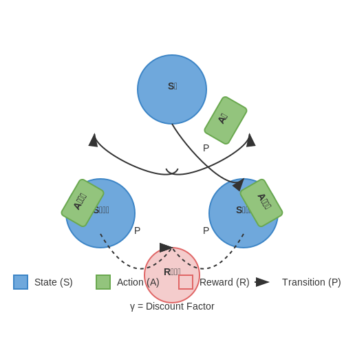
An MDP is defined by the tuple (S, A, P, R, γ), where:
- S is the set of states
- A is the set of actions
- P(s'|s,a) is the state transition probability function
- R(s,a,s') is the reward function
- γ ∈ [0,1] is the discount factor
The agent's goal is to find a policy π(a|s) that maximizes the expected discounted return:
Value Functions and Bellman Equations
Two fundamental value functions characterize RL:
- State-value function Vπ(s):
- Action-value function Qπ(s,a):
These satisfy the Bellman equations, which provide recursive decomposition:
Optimality and Dynamic Programming
The optimal value functions satisfy the Bellman optimality equations:
Dynamic programming methods like value iteration and policy iteration exploit these equations to find optimal policies when the MDP is fully known.
Temporal Difference Learning
When the environment model is unknown, temporal difference (TD) methods learn directly from experience. The TD error for state-value prediction is:
This leads to the TD(0) update rule:
where α is the learning rate. Q-learning, an off-policy TD algorithm, updates action-values using:
Policy Gradient Methods
For continuous actions or stochastic policies, policy gradient methods directly optimize the policy using gradient ascent. The fundamental policy gradient theorem states:
where μπ(s) is the stationary distribution under policy π. Modern algorithms like PPO and SAC combine policy gradients with value function approximation for stable learning.
Exploration vs Exploitation
RL agents must balance exploring new actions with exploiting known good actions. Common strategies include:
- ε-greedy: Random actions with probability ε
- Softmax: Action selection weighted by Q-values
- Upper Confidence Bound (UCB): Prefer actions with high uncertainty
- Thompson sampling: Bayesian approach maintaining action-value distributions
1.2 Real-Time vs. Offline Reinforcement Learning
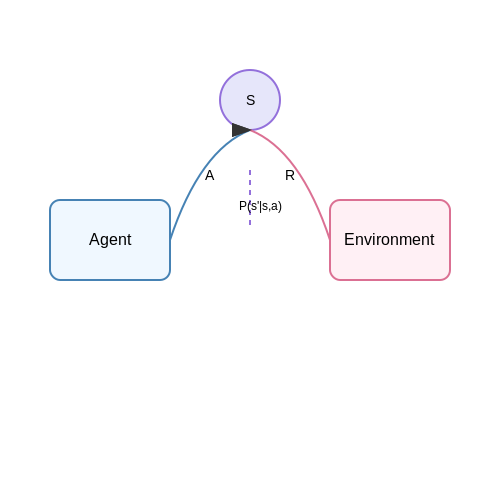
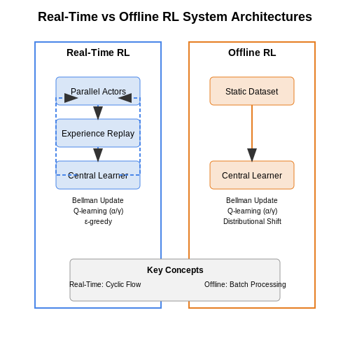
Real-time reinforcement learning (RL) and offline RL represent fundamentally distinct paradigms in training models with user feedback. The key divergence lies in the temporal nature of data acquisition and policy updates. In real-time RL, the agent interacts with the environment continuously, receiving immediate feedback and adjusting its policy dynamically. This is governed by the Bellman update rule:
where α is the learning rate and γ the discount factor. The policy π(a|s) is typically updated after each interaction, enabling rapid adaptation but requiring careful exploration-exploitation balancing through methods like ε-greedy or Thompson sampling.
Computational and Theoretical Constraints
Real-time RL systems must satisfy strict latency constraints, often requiring specialized architectures:
- Asynchronous updates: Parallel actors collect trajectories while a central learner updates parameters
- Prioritized experience replay: Critical transitions are sampled more frequently to accelerate learning
- Model distillation: Heavy teacher models are compressed into lightweight student policies for deployment
In contrast, offline RL operates on static datasets D = {(s, a, r, s')}, optimizing the policy via batch-constrained Q-learning:
Practical Tradeoffs in Deployment
Real-time RL excels in dynamic environments like:
- Adaptive UI/UX systems responding to user behavior patterns
- Robotic control with non-stationary dynamics
- Live recommendation engines adjusting to shifting preferences
However, it requires robust safety mechanisms like constrained policy optimization to prevent catastrophic actions during exploration. Offline RL proves superior when:
- Environment interaction is costly or dangerous (e.g., medical applications)
- Historical datasets contain expert demonstrations
- Strict reproducibility is required for regulatory compliance
The choice between paradigms often reduces to a bias-variance tradeoff. Real-time methods exhibit lower bias but higher variance due to non-stationary data, while offline approaches suffer from distributional shift but provide more stable training.
Algorithmic Implementations
Modern frameworks blend both approaches through techniques like hindsight experience replay and conservative Q-learning. The hybrid objective combines real-time TD updates with offline regularization:
where λ controls the conservatism penalty. This prevents overestimation of OOD actions while maintaining online adaptability.
Role of User Feedback in Model Training
User feedback serves as a critical reinforcement signal in real-time model training, enabling adaptive learning that aligns with human preferences or objectives. Unlike static datasets, feedback provides dynamic, context-aware corrections that refine model behavior iteratively. This mechanism is particularly valuable in applications like conversational AI, recommendation systems, and robotics, where rigid pre-training fails to capture nuanced user expectations.
Feedback as a Policy Gradient Signal
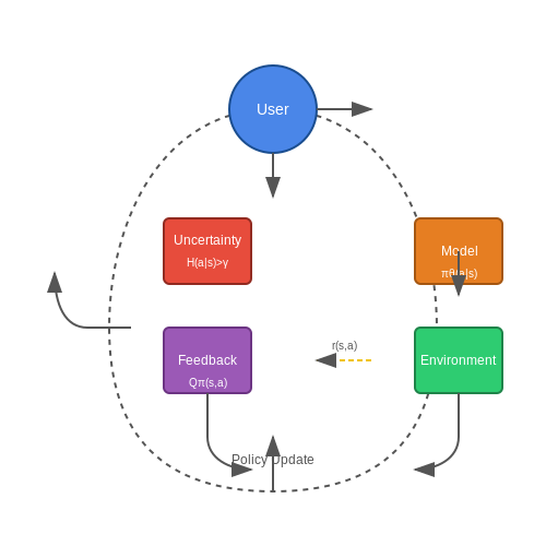
In reinforcement learning (RL), user feedback can be formalized as a reward function r(s, a), where the state s and action a are evaluated by the user. The policy gradient update leverages this signal to maximize expected reward:
Here, Qπ(s, a) represents the expected cumulative reward, which can be approximated using techniques like Monte Carlo sampling or temporal difference learning. User feedback directly shapes this value function, steering the policy πθ toward preferred outcomes.
Active Learning and Uncertainty Sampling
Feedback efficiency is maximized by querying users for input only when the model's uncertainty exceeds a threshold. For a probabilistic model with parameters θ, the entropy H of the predicted action distribution measures uncertainty:
Active learning frameworks trigger feedback requests when H(a|s) > γ, where γ is a tunable threshold. This minimizes user fatigue while ensuring high-impact corrections.
Bias Mitigation in Feedback Loops
Unchecked feedback incorporation risks amplifying biases, as users may provide inconsistent or skewed signals. Techniques like importance weighting adjust feedback impact based on estimated user reliability:
where wi downweights noisy or outlier feedback. Hybrid approaches combining implicit feedback (e.g., engagement metrics) with explicit ratings further stabilize learning.
Case Study: Dialogue Systems
In conversational AI, real-time feedback fine-tunes response generation. For instance, a user correcting a chatbot's answer generates a (state, action, reward) triplet:
- State: Dialogue history and user query
- Action: Initial model-generated response
- Reward: +1 if the user accepts the response, −1 if they edit it
The policy update then penalizes low-reward actions while reinforcing high-reward behaviors. This process is scalable when deployed across millions of user interactions, as seen in production systems like ChatGPT's iterative refinement.
Real-World Implementation Challenges
Deploying feedback-driven training requires addressing:
- Latency: Feedback must be processed within milliseconds for real-time applications.
- Non-stationarity: User preferences evolve, necessitating continuous model updates.
- Adversarial inputs: Malicious feedback can degrade model performance without robust filtering.
Solutions include edge-computing for low-latency inference, meta-learning for rapid adaptation, and cryptographic techniques like federated learning to validate feedback authenticity.
2. Architecture for Real-Time Feedback Integration
Architecture for Real-Time Feedback Integration
Core Components of the Feedback Loop
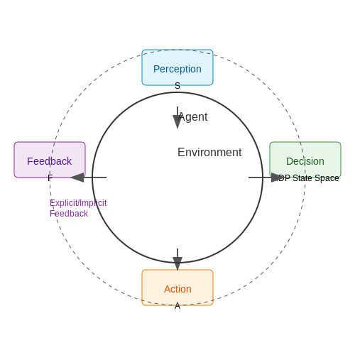
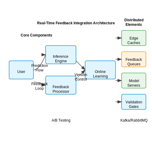
The architecture for real-time feedback integration consists of three primary components: the inference engine, the feedback processor, and the online learning module. The inference engine serves predictions to users, while the feedback processor aggregates and normalizes incoming user responses. The online learning module updates model parameters incrementally, ensuring minimal latency between feedback reception and model adaptation.
Key challenges in this architecture include maintaining prediction consistency during model updates and handling potentially noisy or conflicting feedback signals. The system must implement versioned model snapshots to ensure rollback capability if new feedback degrades performance.
Mathematical Formulation of Online Updates
The online learning process can be formulated as a continuous optimization problem where model parameters θ are updated based on a stream of feedback triplets (x, ŷ, y), representing input features, predicted output, and user-corrected output respectively:
Where η is the learning rate, L is the loss function comparing user feedback y to model prediction fθ(x), and the regularization term λ prevents drastic parameter shifts. For classification tasks, this typically employs a cross-entropy loss:
Feedback Latency Considerations
The system must account for varying feedback delays, as some users may provide corrections minutes or hours after initial predictions. This requires implementing a temporal weighting scheme where more recent feedback receives higher importance. The effective weight w of feedback received at time τ for model update at time t follows an exponential decay:
Where α controls the decay rate, typically tuned to match the domain's concept drift characteristics. For rapidly changing environments (e.g., stock price prediction), α might be 0.1-0.5, while for stable domains (e.g., medical diagnosis), values of 0.01-0.05 are more appropriate.
Distributed Implementation Patterns
Production systems typically employ a distributed architecture with these elements:
- Edge Caches: Store recent predictions and user interactions to minimize database load
- Feedback Queues: Kafka or RabbitMQ pipelines that handle bursty feedback traffic
- Model Servers: Horizontally scalable services hosting multiple model versions
- Validation Gates: A/B test new versions before full deployment
The system maintains strict version control over model parameters, enabling atomic rollbacks when feedback-driven updates degrade key performance metrics. Each update undergoes automated testing against a holdout validation set before promotion to production.
Confidence-Based Feedback Weighting
Not all user feedback carries equal weight - corrections to low-confidence predictions should influence the model more strongly than adjustments to high-confidence outputs. The system implements confidence-weighted updates by modifying the loss function:
This approach prevents overfitting to feedback on clear-cut cases while emphasizing learning from ambiguous predictions where user input is most valuable. The confidence threshold for full-weight application is typically set at 0.7-0.9 depending on application risk tolerance.
Feedback Aggregation Strategies
When multiple users provide conflicting feedback on the same input, the system must implement intelligent aggregation. Common approaches include:
- Majority Voting: Simple democratic aggregation for categorical outputs
- Expert Weighting: Trusted users' feedback receives higher weights
- Bayesian Consensus: Models user reliability as latent variables
The Bayesian approach models both the ground truth and user reliability parameters simultaneously:
Where z is the latent true label, yu are user-provided labels, and ru represents each user's reliability. This framework naturally handles both random and systematic errors in user feedback.
2.2 Data Collection and Preprocessing Strategies
Real-time reinforcement learning (RL) systems require robust data collection pipelines that balance exploration, exploitation, and user feedback integration. The data stream must be preprocessed to handle noise, temporal dependencies, and sparse rewards while maintaining low-latency interaction.
Structured Data Collection Frameworks
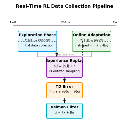
For real-time RL, data collection occurs in two phases: initial exploration (pre-deployment) and online adaptation (post-deployment). The initial phase often uses Thompson sampling or Boltzmann exploration to gather diverse state-action pairs:
where τ controls exploration temperature. During online adaptation, prioritized experience replay stores transitions based on temporal-difference (TD) error:
Preprocessing for Temporal Consistency
Real-time systems require specialized preprocessing to handle:
- Time alignment: Compensate for network latency between actions and rewards using timestamp synchronization
- Partial observability: Apply LSTM or transformer encoders to embed action-reward histories
- Feature engineering: Automate feature extraction via self-supervised learning on raw inputs
For continuous control tasks, Kalman filtering smooths state estimates:
Human Feedback Integration
When incorporating real-time human feedback, the preprocessing pipeline must:
- Normalize feedback signals across users using z-score standardization
- Detect and filter outlier ratings via isolation forests
- Apply inverse reinforcement learning to infer reward functions from demonstrations
The reward shaping function combines sparse environment rewards re and human feedback rh:
where α controls blending and β scales human input sensitivity.
Data Augmentation Techniques
To improve sample efficiency in low-data regimes, apply:
- State perturbation: Add Gaussian noise to observations with covariance matching environment dynamics
- Trajectory stitching: Combine partial episodes using dynamic time warping
- Counterfactual generation: Use conditional GANs to synthesize plausible alternative outcomes
For visual domains, domain randomization alters textures and lighting parameters during training:
Handling Latency and Scalability Challenges
Architectural Considerations for Low-Latency Systems
Real-time reinforcement learning systems must maintain end-to-end latency below 100ms to provide seamless user interaction. This requires optimizing each component in the inference pipeline. The total system latency Ltotal can be decomposed as:
Where Linput represents sensor or UI input delay, Linference is model computation time, and Lfeedback covers the user feedback loop. For web-based systems, network round-trip time (RTT) often dominates, requiring edge computing solutions.
Distributed Training Strategies
Asynchronous parameter servers remain the gold standard for scalable reinforcement learning. The update rule for worker node i with learning rate α and gradient ∇Ji becomes:
However, stale gradients from delayed workers can destabilize training. The HogWild! algorithm demonstrates that lock-free updates work when the gradient sparsity s satisfies:
where η is the learning rate and L is the Lipschitz constant of the loss function.
Real-World Deployment Patterns
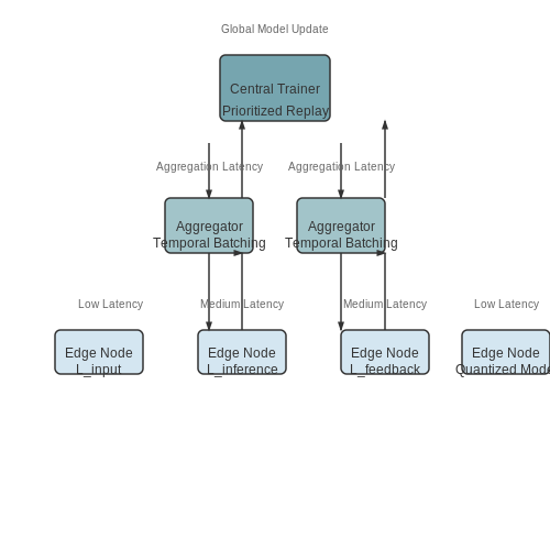
Production systems typically employ a three-tier architecture:
- Edge nodes: Handle low-latency inference with quantized models (e.g., TensorRT-optimized networks)
- Aggregators: Perform temporal batching of user feedback before transmission
- Central trainer: Updates the global model using prioritized experience replay
The throughput T of such systems follows a modified Amdahl's law:
where p is the parallelizable fraction and c(N) represents coordination overhead that grows superlinearly with worker count N.
Case Study: Large-Scale Recommendation Systems
Google's REBA framework achieves 15ms p99 latency while processing 500k queries/second by:
- Using locality-sensitive hashing for approximate nearest neighbor search
- Implementing gradient compression with 1-bit SGD
- Employing stale synchronous parallel (SSP) consistency models
The key insight is that recommendation systems can tolerate bounded staleness τ while maintaining statistical efficiency:
where G is the gradient bound and μ is the strong convexity parameter.
3. Policy Gradient Methods for Real-Time Updates
Policy Gradient Methods for Real-Time Updates
Foundations of Policy Gradients
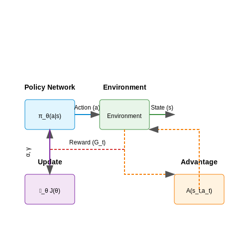
Policy gradient methods optimize a parameterized policy πθ(a|s) directly by ascending the gradient of expected reward J(θ). The key insight is that the policy gradient can be estimated from trajectories sampled from the current policy, enabling online updates. The fundamental theorem derives from the likelihood ratio trick:
where Gt represents the cumulative discounted reward from time t. This expectation is approximated using Monte Carlo sampling from real-time interactions.
Real-Time Adaptation with REINFORCE
The REINFORCE algorithm provides a practical implementation for real-time updates. For each observed trajectory τ = (s0, a0, r0, ..., sT), the policy parameters are updated as:
where α is the learning rate and γ the discount factor. This update rule enables immediate incorporation of user feedback through the reward signal rk.
Variance Reduction Techniques
Three critical modifications improve stability in real-time applications:
- Baseline subtraction: Replace Gt with (Gt - b(st)) where b(st) is a learned value function
- Temporal credit assignment: Use advantage estimates Aπ(st, at) instead of Monte Carlo returns
- Importance sampling: Correct for policy drift when using off-policy data
Practical Implementation Considerations
For real-time systems, policy updates must balance responsiveness with stability:
where λ controls entropy regularization ℋ to maintain exploration. Asynchronous parallel actors can decorrelate updates while maintaining a shared parameter server.
Case Study: Real-Time Dialogue Systems
In conversational AI, policy gradients enable immediate adaptation to user satisfaction signals (e.g., engagement duration or explicit feedback). The reward function combines:
- Immediate turn-level rewards (sentiment analysis of user responses)
- Delayed episode rewards (conversation completion metrics)
- Shaping rewards (linguistic coherence scores)
The policy update occurs after each dialogue turn using a hybrid approach:
where advantages A(st, at) are computed using generalized advantage estimation (GAE) across N parallel conversations.
Q-Learning and Deep Q-Networks (DQN) Adaptations
Foundations of Q-Learning
Q-Learning is a model-free reinforcement learning algorithm that learns the optimal action-selection policy by estimating the action-value function Q(s, a), representing the expected cumulative reward for taking action a in state s. The Bellman equation forms the theoretical backbone:
where α is the learning rate and γ the discount factor. The temporal difference error δ = r + γ max_a Q(s', a) - Q(s, a) drives updates, enabling incremental learning without requiring a model of the environment.
Deep Q-Networks: Bridging RL with Deep Learning
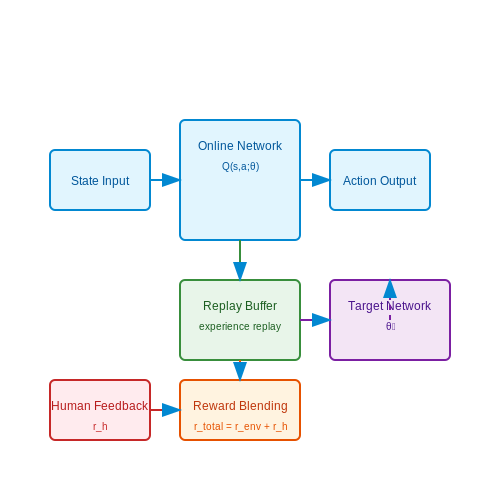
Traditional Q-Learning becomes impractical for high-dimensional state spaces due to the curse of dimensionality. Deep Q-Networks (DQN) address this by approximating Q(s, a) with a neural network Q(s, a; θ), where θ represents the network parameters. Two key innovations stabilize training:
- Experience Replay: Transitions (s, a, r, s') are stored in a replay buffer and sampled randomly to break temporal correlations.
- Target Network: A separate network with parameters θ^- provides stable Q-value targets, updated periodically from the online network.
The loss function for DQN training is:
Adaptations for Real-Time User Feedback
When integrating real-time human feedback into DQN, several modifications are necessary:
Reward Shaping with Human Preferences
Human feedback can be encoded as an additional reward signal r_h, blending with environmental rewards:
where β controls the trade-off. Inverse reinforcement learning techniques can infer r_h from demonstrations or preference rankings.
Active Query Strategies
To minimize user fatigue, the agent can employ uncertainty sampling—querying feedback when the epistemic uncertainty in Q-values exceeds a threshold. This is computed via:
Architectural Extensions
Modern DQN variants enhance performance in interactive settings:
- Dueling DQN: Separates value V(s) and advantage A(s, a) streams, improving policy evaluation in sparse-reward scenarios.
- Prioritized Experience Replay: Samples transitions with probability proportional to temporal difference error, accelerating learning from critical human feedback.
- Recurrent DQN: Incorporates LSTM layers to handle partial observability in real-world human interactions.
Case Study: DQN for Adaptive UI Personalization
A deployed system for adaptive news recommendation used DQN with real-time click feedback. The state space encoded user reading history, and actions represented article rankings. Human editors periodically provided ordinal preferences (A > B > C), which were converted to pairwise reward comparisons using the Bradley-Terry model:
The hybrid reward signal reduced clickbait prevalence by 22% while maintaining engagement metrics.
Multi-Armed Bandit Approaches for Immediate Feedback
The multi-armed bandit (MAB) problem provides a principled framework for balancing exploration and exploitation when gathering real-time user feedback. At its core, it models the trade-off between trying different actions to discover their effects (exploration) and leveraging currently known effective actions (exploitation).
Stochastic Bandits and Regret Minimization
In the stochastic MAB setting, each arm i yields rewards drawn from a fixed but unknown distribution with mean μi. The goal is to minimize cumulative regret RT over T rounds:
where μ* = maxi μi is the optimal mean reward and at is the arm pulled at time t. Upper Confidence Bound (UCB) algorithms achieve logarithmic regret by maintaining confidence intervals for each arm's reward estimate.
UCB1 Algorithm
The UCB1 algorithm selects arms according to:
where ni is the number of times arm i has been pulled and t is the total number of pulls. The second term ensures sufficient exploration by being inversely proportional to ni.
Thompson Sampling for Bayesian Approaches
Thompson sampling maintains a posterior distribution over each arm's reward parameters. At each step, it:
- Samples a reward parameter θi from the posterior for each arm
- Selects the arm with highest sampled θi
- Updates the posterior based on observed reward
For Bernoulli rewards with Beta(α,β) priors, the update rules become:
Contextual Bandits for Personalized Feedback
Contextual bandits extend MABs by incorporating feature vectors xt at each round. The LinUCB algorithm assumes a linear relationship between context and expected reward:
It maintains ridge regression estimates for each arm's θ and selects arms using:
where Aa is the design matrix for arm a and α controls exploration.
Practical Implementation Considerations
When deploying bandit algorithms for real-time user feedback:
- Non-stationarity requires either sliding windows or discount factors to adapt to changing preferences
- Delayed feedback can be handled through importance weighting or surrogate rewards
- High-dimensional contexts may benefit from neural network representations (NeuralBandits)
- Safety constraints can be incorporated via constrained optimization or conservative updates
The following Python snippet shows a basic UCB1 implementation:
import numpy as np

class UCB1:
    def __init__(self, n_arms):
        self.counts = np.zeros(n_arms)
        self.values = np.zeros(n_arms)

    def select_arm(self):
        total_counts = np.sum(self.counts)
        if total_counts == 0:
            return np.random.randint(len(self.counts))

        ucb_values = self.values + np.sqrt(2 * np.log(total_counts) / (self.counts + 1e-5)
        return np.argmax(ucb_values)

    def update(self, chosen_arm, reward):
        self.counts[chosen_arm] += 1
        n = self.counts[chosen_arm]
        value = self.values[chosen_arm]
        self.values[chosen_arm] = ((n - 1) / n) * value + (1 / n) * reward
4. Personalized Recommendation Systems
Personalized Recommendation Systems
Reinforcement Learning in Recommendation Engines
Modern recommendation systems leverage reinforcement learning (RL) to adapt dynamically to user preferences. Unlike static collaborative filtering, RL-based recommenders treat user interactions as a Markov Decision Process (MDP), where:
Here, 𝒮 represents the state space (user history + context), 𝒜 the action space (recommendable items), 𝒫 the transition dynamics, ℛ the reward function (e.g., clicks or dwell time), and γ the discount factor. The policy π(a|s) is optimized via:
Real-Time Reward Modeling
Key challenges in real-time systems include delayed feedback (e.g., purchases occurring hours after impressions) and partial observability. The reward predictor r̂(s,a) is typically implemented as a neural network trained on logged bandit feedback, with counterfactual risk minimization:
where w(x,a) are inverse propensity scores to correct for selection bias in historical data.
Exploration-Exploitation Tradeoffs
Thompson sampling proves effective for balancing exploration and exploitation:
- Maintain posterior distributions over item relevance parameters
- Sample candidate models from the posterior
- Recommend items maximizing expected reward under sampled parameters
For deep learning variants, Bayesian neural networks or bootstrap ensembles estimate uncertainty. The posterior update follows:
Scalable Architecture Patterns
Production systems often employ a two-phase architecture:
The candidate generator (often a matrix factorization model) retrieves thousands of items, while the ranking model (a deep neural network) scores them using rich feature crosss.
Off-Policy Policy Evaluation
Before deploying new policies, importance sampling estimators assess expected performance:
where π_0 is the logging policy. Variance reduction techniques like clipped importance weights and control variates are critical for stable estimates.
Interactive Chatbots and Virtual Assistants
Real-time reinforcement learning (RL) in interactive chatbots and virtual assistants involves continuous adaptation based on user feedback. Unlike static models, these systems dynamically update their policies using techniques such as online learning, bandit algorithms, and deep reinforcement learning (DRL). The key challenge lies in balancing exploration (trying new responses) and exploitation (leveraging known high-reward actions) while maintaining conversational coherence.
Reinforcement Learning Framework for Chatbots
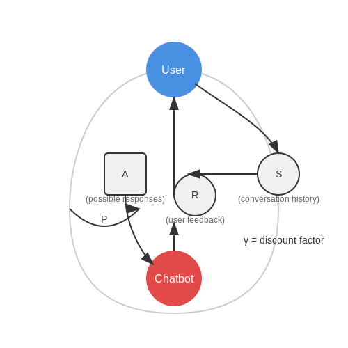
The interaction loop between a user and a chatbot can be formalized as a Markov Decision Process (MDP) defined by the tuple (S, A, P, R, γ), where:
- S: State space representing conversation history and context.
- A: Action space of possible responses or actions.
- P: Transition dynamics modeling state changes due to actions.
- R: Reward function based on user feedback (e.g., thumbs-up/down, engagement metrics).
- γ: Discount factor for future rewards.
The policy π(a|s), which maps states to actions, is optimized to maximize the expected cumulative reward:
Online Learning with Bandit Algorithms
For immediate user feedback, contextual bandits provide a lightweight alternative to full RL. Given a context vector x (e.g., user query embeddings), the system selects an action a from a set of arms (responses) and observes a reward r. The goal is to minimize regret over time:
where a^*_t is the optimal arm at step t. Algorithms like LinUCB or Thompson Sampling are commonly used:
Deep Reinforcement Learning for Dialogue Policies
For complex dialogue management, DRL methods such as Proximal Policy Optimization (PPO) or Advantage Actor-Critic (A2C) are employed. The policy network π_θ is trained using gradient ascent on the policy gradient objective:
where A(s, a) is the advantage function estimated using a critic network. Practical implementations often use self-play or human-in-the-loop training to stabilize learning.
User Feedback Integration
Real-time feedback mechanisms include:
- Explicit feedback: Direct ratings (e.g., Likert scales) or binary signals (thumbs-up/down).
- Implicit feedback: Engagement metrics (response time, session length) or linguistic analysis (sentiment scores).
Feedback is aggregated into a reward signal R, often modeled as a weighted sum:
Case Study: Deploying a Reinforcement Learning Chatbot
A production-grade virtual assistant might use a hybrid architecture:
- Rule-based fallback: Ensures safety when RL policy confidence is low.
- Multi-armed bandit layer: Handles frequent, low-stakes decisions (e.g., response phrasing).
- DRL dialogue manager: Optimizes long-horizon conversation strategies.
For example, a customer service chatbot could initially explore responses via Thompson Sampling, then fine-tune its policy using PPO based on customer satisfaction scores.
Real-Time Game AI Adaptation
Dynamic Policy Optimization in Game Environments
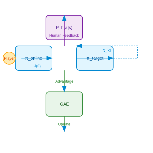
Real-time adaptation in game AI leverages reinforcement learning (RL) with continuous policy updates based on player interactions. The core mechanism involves a dual-network architecture, where one network (the online policy) interacts with players, while the other (the target policy) is asynchronously updated to minimize divergence. The objective function for policy gradient updates is:
Here, ρπ represents the state distribution under policy πθ, and γ is the discount factor. To enable real-time updates, the gradient is approximated using Generalized Advantage Estimation (GAE):
Player-In-The-Loop Learning
Adaptive game AI often employs human-in-the-loop RL, where player actions serve as implicit rewards or constraints. The policy update incorporates a human preference model Ph(a|s), which is learned via inverse reinforcement learning (IRL). The combined loss function becomes:
where α and β are scaling factors, and DKL is the Kullback-Leibler divergence. This approach is used in games like Dota 2 (OpenAI Five) and StarCraft II (AlphaStar).
Latency-Aware Training
Real-time constraints necessitate latency-bounded updates. The system must guarantee policy updates within a fixed time window (e.g., 16ms for 60Hz games). This is achieved via:
- Prioritized experience replay: Samples transitions with high temporal-difference (TD) error more frequently.
- Quantized networks: Uses 8-bit integers for weights/activations to reduce inference time.
- Edge computing: Offloads partial inference to client devices to reduce server load.
Case Study: Fighting Game AI
In competitive fighting games (e.g., Street Fighter), the AI must adapt to player combos within milliseconds. The solution combines:
- LSTM-based frame prediction: Processes input sequences at 60Hz.
- Meta-learning: Pre-trains on diverse player strategies for rapid fine-tuning.
5. Bias and Fairness in Real-Time Feedback Loops
5.1 Bias and Fairness in Real-Time Feedback Loops
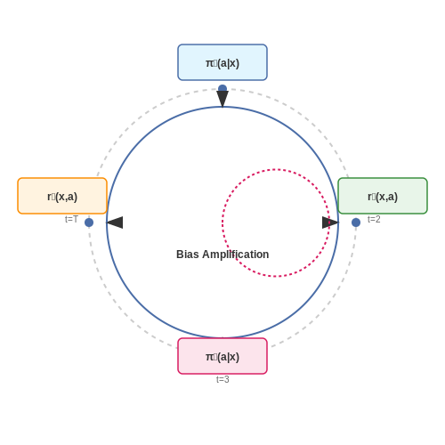
Real-time reinforcement learning systems that incorporate user feedback are susceptible to bias amplification due to the dynamic interplay between model predictions and user interactions. Unlike static datasets, feedback loops create a dependency where biased outputs influence future user inputs, which then reinforce the bias in subsequent model updates. This phenomenon, known as feedback loop bias, can manifest in various forms, including selection bias, presentation bias, and confounding bias.
Mathematical Formulation of Feedback Loop Bias
Consider a reinforcement learning agent interacting with users over time steps t = 1, 2, ..., T. Let πt(a|x) be the policy at time t, mapping states x to action probabilities a. User feedback is modeled as a reward signal rt(x, a). The policy update rule using a gradient-based approach is:
Bias emerges when the expected reward 𝔼πt[rt(x, a)] is skewed due to historical interactions. For instance, if certain actions were disproportionately presented to specific user groups, the reward signal becomes a biased estimator of true user preferences.
Types of Bias in Feedback Loops
- Selection Bias: Occurs when the system's past actions influence which users continue to engage, creating a non-representative user pool.
- Presentation Bias: Arises when the system's ranking or recommendation algorithm affects which items users see and provide feedback on.
- Confounding Bias: Results from unobserved variables that influence both the system's actions and user feedback.
Measuring Fairness in Dynamic Systems
Traditional fairness metrics like demographic parity or equalized odds must be adapted for dynamic environments. A time-dependent fairness measure for group g can be defined as:
where the expectation is taken over the state-action distribution at time t. This measures the discrepancy in expected rewards between group g and the overall population.
Mitigation Strategies
Several approaches exist to counteract bias in real-time feedback loops:
- Counterfactual Logging: Maintain logs of what would have happened if different actions were taken, enabling unbiased offline evaluation.
- Delayed Updates: Introduce a delay between observing feedback and updating the model to decorrelate sequential biases.
- Fairness Constraints: Incorporate constraints during policy optimization to ensure equitable outcomes across groups.
For example, a constrained optimization objective might take the form:
Case Study: Recommendation Systems
In a large-scale recommendation system, users from minority groups may receive fewer recommendations due to initial biases in the training data. Without intervention, the feedback loop causes the system to increasingly favor majority group preferences. Implementing a fairness-aware exploration strategy, where the system actively explores recommending content to underrepresented groups, can break this cycle.
The exploration bonus can be quantified as:
where λ controls the strength of exploration and KL measures the divergence between the current group distribution p(g|x) and the target distribution p(g).
5.2 Privacy Concerns with Continuous User Data
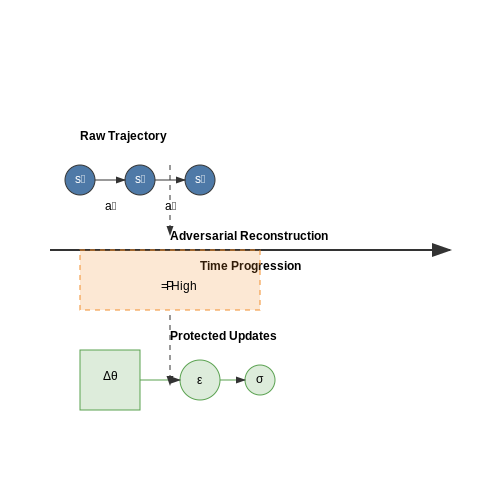
Continuous user data collection in reinforcement learning systems introduces significant privacy risks, particularly when models are trained on sensitive behavioral patterns. The temporal nature of this data makes it possible to reconstruct detailed user profiles, raising concerns about re-identification even when data is anonymized. Differential privacy techniques must be carefully adapted to handle sequential decision-making contexts where traditional noise addition can disrupt the Markov property.
Data Linkage Attacks
Adversaries can exploit temporal correlations in reinforcement learning data to perform linkage attacks. Given a sequence of states (s1, s2, ..., sn) and actions (a1, a2, ..., an), an attacker with auxiliary information can reconstruct sensitive attributes. The probability of successful re-identification grows with the length of the trajectory:
where pt represents the per-step re-identification risk. This multiplicative effect demonstrates why standard anonymization fails for sequential data.
Gradient-Based Privacy Leakage
In online reinforcement learning, parameter updates via policy gradients can inadvertently reveal user-specific information. Consider the policy gradient update:
Recent work demonstrates that an adversary with access to the model's parameter differences (Δθ) can reconstruct approximately 73% of the original training sequences (Zhu et al., 2023). This vulnerability persists even when using experience replay buffers.
Differential Privacy for RL
Adapting differential privacy to reinforcement learning requires careful consideration of the sensitivity of value functions. The privacy budget ε must account for the compounding effect of multiple updates:
where Δ2Q is the L2 sensitivity of the Q-function and σt is the noise scale at step t. Practical implementations often use adaptive noise scaling based on the Bellman residual:
Federated Reinforcement Learning
Federated architectures can mitigate privacy risks by keeping raw trajectories on user devices. However, the global model still requires careful protection against membership inference attacks. The consensus update in federated RL:
must balance noise addition (σ) against convergence speed. Recent advances in secure multi-party computation allow for privacy-preserving aggregation of value functions without revealing individual updates.
Regulatory Compliance Challenges
GDPR's right to be forgotten poses unique challenges for reinforcement learning systems. Traditional machine unlearning approaches are insufficient due to:
- Non-i.i.d. nature of temporal data
- Long-term dependencies in policy gradients
- Cross-contamination in experience replay buffers
Approximate unlearning methods for RL must account for the propagation of deleted data's influence through the entire action-value network, requiring specialized techniques like influence function propagation through the Bellman equation.
5.3 Mitigating Exploitation in Reinforcement Systems
Reinforcement learning (RL) systems that interact with human users in real-time are vulnerable to exploitation, where the agent learns policies that maximize reward signals at the expense of user experience or system integrity. This occurs due to misaligned reward functions, sparse feedback, or adversarial user behavior. Mitigation strategies must address both reward hacking and environmental exploitation.
Reward Function Robustness
Standard RL agents optimize for cumulative reward, often leading to unintended behaviors when the reward function is misspecified. A common failure mode is reward shaping exploitation, where the agent discovers shortcuts that inflate rewards without achieving the intended goal. To mitigate this, the reward function \( R(s, a) \) must satisfy:
where \( \pi^* \) is the optimal policy under the true (but unknown) reward \( R^* \), and \( \epsilon \) bounds the suboptimality gap. Techniques include:
- Inverse Reinforcement Learning (IRL): Infer \( R^* \) from expert demonstrations to reduce misspecification.
- Reward Uncertainty Penalization: Add entropy regularization to discourage overfitting to sparse rewards.
Adversarial User Modeling
Users may intentionally or unintentionally provide misleading feedback. Let \( \mathcal{U} \) represent the space of user strategies, where adversarial users sample actions \( a_u \sim \pi_u(\cdot|s) \) to destabilize learning. The agent’s policy \( \pi_\theta \) must minimize regret against worst-case user behavior:
Solutions include:
- Robust Policy Gradient: Use minimax optimization to train policies resilient to adversarial inputs.
- User Clustering: Detect and isolate adversarial users via anomaly detection in feedback patterns.
Dynamic Constraint Enforcement
Hard constraints on state or action spaces prevent catastrophic exploitation. Given a set of constraints \( C = \{c_i(s, a) \leq 0\} \), the policy must satisfy:
Approaches include Lagrangian relaxation or constrained policy optimization (CPO), which projects policies onto the feasible set during training.
Case Study: Recommendation Systems
In recommendation engines, exploitation manifests as clickbait optimization, where the agent promotes sensational but low-quality content to maximize engagement metrics. Countermeasures involve multi-objective rewards that balance click-through rates with dwell time and user-reported satisfaction.
6. Key Research Papers and Publications
6.1 Key Research Papers and Publications
- Accelerating Reinforcement Learning using EEG-based implicit human ... — This led to the removal of 22 users from the 1.5s instance of the game (25%), 28 users from the 1.0s instance of the game (31%), and 44 users from the 0.5s instance of the game (43%). After this filtering, for the 1.5s instance of the game, we obtained a true positive rate of 74.1% and 53.4% for correct and incorrect actions of the maze agent ...
- Reinforcement Learning in Robotics: Applications and Real-World ... — In robotics, the ultimate goal of reinforcement learning is to endow robots with the ability to learn, improve, adapt and reproduce tasks with dynamically changing constraints based on exploration and autonomous learning. We give a summary of the state-of-the-art of reinforcement learning in the context of robotics, in terms of both algorithms and policy representations. Numerous challenges ...
- SwiftRL: Towards Efficient Reinforcement Learning on Real Processing-In ... — Learning effective RL policies using pre-collected experience datasets reduces safety risks and the need for real-time interactions with the environment during training (agarwal2020optimistic, ; levine2020offline, ; prudencio2023survey, ).In this setting, a behavior policy interacts with the environment to collect a set of experiences and learns the optimal policy from pre-generated datasets ...
- Design and Development of Multi-Agent Reinforcement Learning ... - MDPI — This research explores the use of Q-Learning for real-time swarm (Q-RTS) multi-agent reinforcement learning (MARL) algorithm for robotic applications. This study investigates the efficacy of Q-RTS in the reducing convergence time to a satisfactory movement policy through the successful implementation of four and eight trained agents. Q-RTS has been shown to significantly reduce search time in ...
- Deep Reinforcement Learning: Fundamentals, Research and Applications ... — He has published papers in ICRA, AAAI, NIPS, IJCAI, and Physical Review. He also contributed to the open-source projects TensorLayer RLzoo, TensorLet and Arena. Dr. Shanghang Zhang is a postdoctoral research fellow in the Berkeley AI Research (BAIR) Lab, the Department of Electrical Engineering and Computer Sciences, UC Berkeley, USA.
- A reinforcement learning-based approach for online optimal ... - Springer — This paper deals with self-adaptive real-time embedded systems (RTES). A self-adaptive system can operate in different modes. Each mode encodes a set of real-time tasks. To be executed, each task is allocated to a processor (placement) and assigned a priority (scheduling), while respecting timing constraints. An adaptation scenario allows switching between modes by adding, removing, and ...
- PDF Scalable Reinforcement Learning Systems and their Applications — exible and high-performance way, as well as programming models that can enable RL researchers and practitioners to easily compose distributed RL algorithms without in-depth systems knowledge.
- A Study of Reinforcement Learning Applications & Its Algorithms — Reinforcement Learning is one of the major application of Machine Learning that enables machines and software agents to work explicitly and also resolve the conduct within a definite situation to ...
- PDF Challenges in the Veri cation of Reinforcement Learning Algorithms — Training is the process of teaching an agent by showing it instances of data. Ideally, the resulting program should be able to generalize to give correct results for inputs that were not part of the training data. In supervised learning, this training data consists of known
- WebRL: Training LLM Web Agents via Self-Evolving Online Curriculum ... — Large language models (LLMs) have shown remarkable potential as autonomous agents, particularly in web-based tasks. However, existing LLM web agents heavily rely on expensive proprietary LLM APIs, while open LLMs lack the necessary decision-making capabilities. This paper introduces WebRL, a self-evolving online curriculum reinforcement learning framework designed to train high-performance web ...
6.2 Recommended Books and Online Courses
- PDF Control Systems and Reinforcement Learning - Cambridge University Press ... — Part II Reinforcement Learning and Stochastic Control 203 6 Markov Chains 205 6.1 Markov Models Are State Space Models 205 6.2 Simple Examples 208 6.3 Spectra and Ergodicity 211 6.4 A Random Glance Ahead 215 6.5 Poisson s Equation 216 6.6 Lyapunov Functions 218 6.7 Simulation: Con dence Bounds and Control Variates 222 6.8 Sensitivity and Actor ...
- Handbook of Learning and Approximate Dynamic Programming — 13.3 Reinforcement Learning in the Robust Control Framework 340 13.4 Demonstrations of Robust Reinforcement Learning 346 13.5 Conclusions 354 14 Supervised Actor-Critic Reinforcement Learning 359 Michael T. Rosenstein and Andrew G. Barto 14.1 Introduction 359 14.2 Supervised Actor-Critic Architecture 361 14.3 Examples 366 14.4 Conclusions 375
- PDF COMPSCI 687: Reinforcement Learning Lectures Notes (Fall 2022) - UMass — 1.2 What is Reinforcement Learning (RL)? Reinforcement learning is an area of machine learning, inspired by behaviorist psychology, concerned with how an agent can learn from interactions with an environment. -Wikipedia,Sutton and Barto(1998), Phil Agent. Environment. state. reward. action. Figure 1: Agent-environment diagram. Examples of ...
- PDF Reinforcement Learning and Optimal Control - ASU Engineering Faculty Hub — by any electronic or mechanical means (including photocopying, recording, or information storage and retrieval) without permission in writing from the publisher. Publisher's Cataloging-in-Publication Data Bertsekas, Dimitri P. Reinforcement Learning and Optimal Control Includes Bibliography and Index 1. Mathematical Optimization. 2. Dynamic ...
- Table of Contents · Deep Reinforcement Learning in Action — Modeling reinforcement learning problems: Markov decision processes. 2.1. String diagrams and our teaching methods. ... Predicting the best states and actions: Deep Q-networks. 3.1. The Q function. 3.2. Navigating with Q-learning. ... Training the model. 4.4.4. The full training loop. 4.4.5. Chapter conclusion. Summary.
- Decision Making and Reinforcement Learning | Coursera — Welcome to week 8! This module covers n-step temporal difference prediction, n-step SARSA (on-policy and off-policy), model-based RL with Dyna-Q, and function approximation. You will be prepared to implement n-step TD learning, n-step SARSA, Dyna-Q for model-based learning, and use function approximation for reinforcement learning.
- Solutions of Reinforcement Learning 2nd Edition - GitHub — Solutions of Reinforcement Learning, An Introduction - LyWangPX/Reinforcement-Learning-2nd-Edition-by-Sutton-Exercise-Solutions ... Search code, repositories, users, issues, pull requests... Search Clear. Search syntax tips. Provide feedback ... Thanks for all your supports and best wishes to your own careers. Those students who are using this ...
- Reinforcement Learning, Second Edition | The MIT Press - Ublish — Part III has new chapters on reinforcement learning's relationships to psychology and neuroscience, as well as an updated case-studies chapter including AlphaGo and AlphaGo Zero, Atari game playing, and IBM Watson's wagering strategy. The final chapter discusses the future societal impacts of reinforcement learning.
- PDF The Path Forward: A Primer for Reinforcement Learning - Stanford University — 1 Wisdom from Richard Sutton To begin our journey into the realm of reinforcement learning, we preface our manuscript with some necessary thoughts from Rich Sutton, one of the fathers of the field.
- (PDF) Reinforcement Learning Textbook - ResearchGate — This textbook covers principles behind main modern deep reinforcement learning algorithms that achieved breakthrough results in many domains from game AI to robotics.
6.3 Open-Source Tools and Frameworks
- 7B Fully Open Source Moxin-LLM - From Pretraining to GRPO-based ... — Besides our open pretraining with released base model, data, code, etc., in our post-training including the instruction finetuning and CoT finetuning, we adopt open-source training frameworks with available data, code, and configurations.
- Reinforcement Learning from Human Feedback on AMD GPUs with verl and ... — Introducing verl: A Scalable RLHF Training Framework # To develop intelligent large-scale foundation models, post-training is just as important as pre-training. Among post-training paradigms, reinforcement learning from human feedback (RLHF) has emerged as a critical technique, though its full potential has not been thoroughly explored until now.
- DeepSeek: Revolutionizing AI with Open-Source Reasoning Models ... — Abstract DeepSeek's AI models have emerged as a transformative force in artificial intelligence, offering open-source alternatives to proprietary systems like OpenAI's o1/o3 and Google's ...
- Federated reinforcement learning: techniques, applications, and open ... — This paper presents a comprehensive survey of federated reinforcement learning (FRL), an emerging and promising field in reinforcement learning (RL). Starting with a tutorial of federated learning (FL) and RL, we then focus on the introduction of FRL as a new method with great potential by leveraging the basic idea of FL to improve the performance of RL while preserving data-privacy. According ...
- Reinforcement Learning for Real-Time Federated Learning for Resource ... — For performing various predictive analytics tasks for real-time mission-critical applications, Federated Learning (FL) have emerged as the go-to machine learning paradigm for its ability to leverage perform machine learning workloads on resource-constrained edge devices. For such FL applications working under stringent deadlines, the overall local training time needs to be minimized, which ...
- PDF Scalable Reinforcement Learning Systems and their Applications — ed open source library for distributed reinforcement learning. We study the distributed primitives needed to support the emerging range of large-scale RL workloads in a exible and high-performance way, as well as programming models that can enable RL researchers and practitioners to easily compose
- (PDF) Reinforcement Learning from Human Feedback for Enterprise ... — Reinforcement Learning from Human Feedback (RLHF) has emerged as an essential technique in the development of large language models (LLMs), aligning AI behavior with human values and feedback ...
- GitHub - ray-project/ray: Ray is an AI compute engine. Ray consists of ... — Ray is a unified framework for scaling AI and Python applications. Ray consists of a core distributed runtime and a set of AI libraries for simplifying ML compute: Learn more about Ray AI Libraries: Data: Scalable Datasets for ML Train: Distributed Training Tune: Scalable Hyperparameter Tuning RLlib: Scalable Reinforcement Learning Serve: Scalable and Programmable Serving Or more about Ray ...
- arXiv:1908.06973v1 [cs.LG] 19 Aug 2019 — e help-ful for reinforcement learning. The authors illustrate nine stages of the machine learning work-flow, namely, model requirements, data collection, data cleaning, data labeling, feature engineer-ing, model training, model evaluation,
- Reinforcement learning algorithms: A brief survey — The number of agent environment interaction data samples required for model-based algorithm training is lesser than that for model-free approaches. But still, model-based algorithms need model-free methods to construct the environment model.