World Models for Simulated Planning
1. Definition and Core Concepts
World Models for Simulated Planning: Definition and Core Concepts
World models are learned neural network representations that approximate an environment's dynamics, enabling agents to simulate future states and plan actions without direct interaction with the real world. These models capture the joint probability distribution of observations, actions, and rewards:
where st represents the state at time t, at denotes the action taken, and rt is the received reward. The model's predictive capability stems from its ability to compress high-dimensional sensory inputs into a latent space where temporal relationships can be efficiently modeled.
Key Components of World Models
Modern world models typically consist of three neural networks working in concert:
- Variational Autoencoder (VAE): Compresses observations into a latent space zt while preserving essential features for dynamics prediction. The encoder qϕ(zt|ot) and decoder pθ(ot|zt) are trained jointly using the evidence lower bound (ELBO):
- Recurrent State-Space Model (RSSM): Captures temporal dependencies through a combination of deterministic and stochastic latent states. The transition function fψ predicts the next latent state:
- Reward Predictor: Estimates the expected reward r̂t from latent states, enabling value estimation during planning.
Planning in Latent Space
World models enable efficient planning through latent imagination, where agents evaluate action sequences in the compressed representation rather than raw observation space. The planning process typically involves:
- Rolling out multiple trajectories using the learned dynamics model
- Estimating expected returns for each trajectory
- Selecting actions that maximize the predicted return
This approach reduces computational complexity compared to traditional model-based RL methods that operate directly in observation space. The planning horizon H trades off between computational cost and solution quality, with typical values ranging from 10 to 100 steps for complex environments.
Practical Considerations
Effective world model implementation requires addressing several challenges:
- Distributional Shift: The compounding error problem arises when the model's predictions diverge from real environment dynamics during long rollouts. Techniques like scheduled sampling and ensemble methods help mitigate this issue.
- Partial Observability: Environments with hidden state require careful design of the latent representation to maintain sufficient history information.
- Multi-Modality: Stochastic environments benefit from mixture density outputs or latent variable approaches to capture diverse future possibilities.
Recent advances in transformer-based world models demonstrate improved handling of long-range dependencies through self-attention mechanisms, enabling more accurate predictions over extended time horizons. These architectures often replace the traditional RSSM with a transformer that operates directly on the latent sequence:

1.2 Historical Context and Evolution
The concept of world models for simulated planning traces its roots to early developments in artificial intelligence, control theory, and cognitive science. In the 1960s, researchers like Richard Bellman laid the groundwork with dynamic programming and the principle of optimality, formalized as:
where V* represents the optimal value function, R the reward, and P the transition dynamics. This Bellman equation became the theoretical foundation for later model-based reinforcement learning approaches.
Early Symbolic Approaches
In the 1970s-1980s, STRIPS (Stanford Research Institute Problem Solver) introduced symbolic representations of world states and actions, enabling planners to reason about state transitions through first-order logic. The STRIPS operator consisted of:
- Preconditions: Logical conditions required for action execution
- Add effects: New facts added to the world state
- Delete effects: Facts removed from the world state
This formalism allowed for simulated planning through state-space search, though it suffered from combinatorial explosion in complex environments.
Neural Network Revolution
The 2010s saw a paradigm shift with the integration of deep learning. Key developments included:
where neural networks parameterized by θ learned to approximate environment dynamics. The 2018 World Models paper by Ha and Schmidhuber demonstrated how variational autoencoders (VAEs) could compress high-dimensional observations into latent states zt, with a recurrent network predicting zt+1:
This architecture enabled agents to learn compact world models that could be used for planning through techniques like the Cross-Entropy Method (CEM).
Modern Developments
Recent advances have focused on improving world models through:
- Contrastive learning: Learning representations by maximizing mutual information between different views of the same state
- Hierarchical models: Capturing temporal abstractions through multi-scale predictions
- Uncertainty estimation: Using Bayesian neural networks or ensemble methods to quantify model uncertainty
The evolution of world models has been closely tied to improvements in computational power, with modern implementations leveraging parallel simulation across thousands of TPU cores for large-scale planning.

Key Applications in Simulated Planning
Autonomous Robotics and Control
World models enable robots to simulate potential actions before execution, reducing real-world trial-and-error. For instance, a robotic arm can predict the outcome of grasping an object by running thousands of simulated trajectories in a learned latent space. The model minimizes the discrepancy between predicted and actual states using a loss function:
where st is the current state, at the action, and ŝt+1 the predicted next state. This approach is critical in dynamic environments like warehouse automation, where real-time replanning is necessary.
Reinforcement Learning (RL) Acceleration
World models act as surrogate environments for RL agents, allowing off-policy training without costly real-world interactions. The agent learns a policy π(a|s) by interacting with the simulated dynamics model p(s'|s, a). Key steps include:
- Latent Space Rollouts: The agent generates synthetic trajectories by sampling from the learned latent space.
- Policy Gradient Updates: The policy is optimized using Proximal Policy Optimization (PPO) or Soft Actor-Critic (SAC) within the simulated environment.
This method was pivotal in OpenAI's "Mujoco Humanoid" experiments, reducing real-world training samples by 90%.
Industrial Process Optimization
Chemical and manufacturing plants use world models to simulate production line adjustments. A differentiable physics engine predicts outcomes like material flow or thermal distribution, encoded as:
where fθ is the learned dynamics model and ŷ the target metric (e.g., yield efficiency). BASF reported a 12% throughput increase using such models for catalytic reactor optimization.
Medical Treatment Planning
World models simulate patient responses to treatment regimens by integrating electronic health records (EHRs) with pharmacokinetic models. A hybrid architecture combines:
- Graph Neural Networks (GNNs): To model patient-specific metabolic pathways.
- Time-series Predictors: For dose-response forecasting.
For example, a model might predict tumor shrinkage under varying drug combinations, optimizing for:
where R(st, at) quantifies treatment efficacy and side effects.
Climate and Urban Planning
City-scale world models simulate traffic, energy use, and disaster responses. The NVIDIA "Earth-2" initiative uses diffusion models to predict microclimate changes at 1km resolution, solving PDEs in latent space:
where z is the latent representation of atmospheric variables, and gϕ is a neural PDE solver. Such models enable stress-testing urban designs against floods or heatwaves.
2. Neural Network Components
2.1 Neural Network Components
Recurrent Neural Networks (RNNs) for Temporal Dynamics
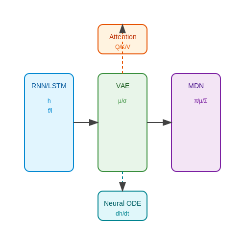
World models rely heavily on recurrent architectures to capture temporal dependencies in sequential data. The core mechanism involves hidden state propagation through time, governed by:
where ht represents the hidden state at time t, σ is a nonlinear activation (typically tanh or ReLU), and Wh, Wx are trainable weight matrices. Long Short-Term Memory (LSTM) variants address vanishing gradients through gating mechanisms:
Variational Autoencoders (VAEs) for Latent Space Learning
The encoder qφ(z|x) maps high-dimensional observations to a latent Gaussian distribution, while the decoder pθ(x|z) reconstructs inputs. The evidence lower bound (ELBO) objective combines reconstruction loss and KL divergence:
where β controls the trade-off between reconstruction fidelity and latent space regularization. Practical implementations often use the reparameterization trick for differentiable sampling: z = μ + σ ⊙ ε with ε ∼ N(0,I).
Mixture Density Networks (MDNs) for Multimodal Prediction
When integrated with RNNs, MDNs model complex conditional distributions by predicting Gaussian mixture parameters:
The network outputs mixture coefficients πk, means μk, and covariance matrices Σk through specialized output heads. Training minimizes the negative log-likelihood:
Attention Mechanisms for Contextual Weighting
Modern world models employ attention to dynamically focus on relevant temporal segments. The scaled dot-product attention computes:
where Q, K, V are learned query, key, and value matrices. Transformer-based variants stack multiple attention heads with layer normalization and residual connections, enabling parallel processing of long sequences.
Neural ODEs for Continuous-Time Dynamics
For systems requiring continuous-time modeling, neural ordinary differential equations parameterize the derivative:
with solutions computed through adaptive numerical integration. The adjoint method enables memory-efficient backpropagation by solving a second ODE for gradients:
where a(t) represents the gradient of the loss with respect to the hidden state.
Latent Space Representation
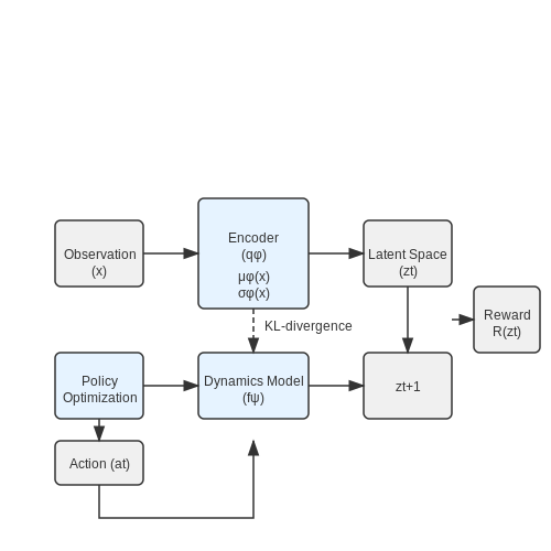
World models leverage latent space representations to encode high-dimensional observations into a compact, structured form that facilitates efficient planning and prediction. The latent space z is typically learned via variational autoencoders (VAEs) or other nonlinear dimensionality reduction techniques, enabling the model to capture essential features while discarding irrelevant noise. This compression is critical for simulating long-horizon trajectories without accumulating errors from raw pixel space.
Mathematical Formulation
The encoder qϕ(z | x) maps an observation x to a probabilistic latent representation z, often modeled as a Gaussian distribution:
where μϕ and σϕ are neural networks parameterized by ϕ. The decoder pθ(x | z) reconstructs observations from latent states, trained to minimize reconstruction loss alongside a KL-divergence term enforcing latent space regularity:
Here, p(z) is a prior (e.g., standard normal), and β controls the trade-off between reconstruction fidelity and latent space structure.
Dynamics in Latent Space
A learned transition model pψ(zt+1 | zt, at) predicts future latent states given current states and actions. For deterministic dynamics, this reduces to:
where fψ is typically a recurrent or feedforward neural network. Stochastic variants use Gaussian transitions or normalizing flows to model uncertainty.
Planning via Latent Optimization
Agents optimize action sequences in latent space by backpropagating through the dynamics model to maximize expected reward R(zt):
Gradient-based methods (e.g., cross-entropy method, model-predictive control) are computationally efficient in this compressed representation compared to pixel-space planning.
Case Study: Dreamer Architecture
The Dreamer algorithm demonstrates latent space planning by training a world model (VAE + recurrent dynamics) and a policy entirely in latent space. This achieves state-of-the-art sample efficiency in reinforcement learning benchmarks by decoupling costly environment interactions from latent imagination.
Dynamics Prediction Mechanisms
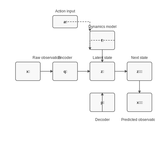
Dynamics prediction in world models involves learning a transition function that maps the current state and action to the next state. This function is typically parameterized as a neural network trained to minimize prediction error. The most common formulation uses a deterministic or stochastic recurrent neural network (RNN) to model state transitions:
where θ represents the learnable parameters of the dynamics model. For stochastic environments, the prediction is often modeled as a Gaussian distribution:
Latent Space Dynamics
Modern approaches operate in learned latent spaces rather than raw observation spaces. The dynamics model predicts transitions between latent states z_t encoded from observations x_t:
This formulation requires joint training of an encoder q_φ(z_t|x_t) and decoder p_ψ(x_t|z_t) alongside the dynamics model. The reconstruction loss ensures the latent space preserves semantically meaningful information.
Architectural Choices
Several neural architectures have proven effective for dynamics prediction:
- Recurrent Networks: LSTMs and GRUs naturally handle sequential prediction but may struggle with long-term dependencies
- Transformers: Self-attention mechanisms excel at capturing long-range dependencies but require careful positional encoding
- Neural ODEs: Continuous-depth models that learn the derivative of state changes rather than discrete transitions
Training Objectives
The dynamics model is typically trained using a combination of:
where the first term minimizes prediction error and the second term (weighted by λ) regularizes the latent space to match the prior dynamics distribution.
Uncertainty Estimation
Effective world models must quantify prediction uncertainty. Common approaches include:
- Ensemble Methods: Training multiple models and measuring disagreement
- Bayesian Neural Networks: Learning distributions over weights
- Normalizing Flows: Modeling complex output distributions
The uncertainty estimates are crucial for planning algorithms to balance exploration and exploitation.
Practical Considerations
Several challenges arise in real-world applications:
- Compounding Errors: Small prediction errors accumulate over long rollouts
- Partial Observability: Many environments require memory beyond the immediate state
- Multi-Modality: Some actions may lead to several distinct plausible futures
Recent advances address these through techniques like scheduled sampling, hierarchical latent spaces, and mixture density outputs.
3. Data Collection and Preprocessing
3.1 Data Collection and Preprocessing
Sensor Data Acquisition
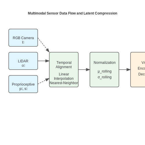
World models rely on high-dimensional sensory inputs, typically collected from simulated or real-world environments. For simulated planning, data is often generated via physics engines such as MuJoCo, PyBullet, or Unity. The raw observations ot at time t may include:
- RGB or depth images (64×64 to 256×256 resolution)
- LIDAR point clouds
- Proprioceptive data (joint angles, velocities)
- Environmental state vectors (object positions, velocities)
where It denotes visual inputs, pt proprioceptive data, and st environmental state variables.
Temporal Downsampling and Alignment
Multimodal sensors often operate at different frequencies (e.g., cameras at 30Hz, proprioception at 1kHz). Temporal alignment is achieved through:
- Linear interpolation for continuous signals (joint angles)
- Nearest-neighbor sampling for discrete events (contact sensors)
Normalization Techniques
Input standardization is critical for training stability. For visual data, pixel values are scaled to [-1, 1] via:
Continuous state variables are normalized using running statistics:
Data Augmentation Strategies
To improve generalization, apply stochastic transformations:
- Visual domain: Random crops, color jitter, and cutout
- Physics domain: Parameter noise (mass, friction coefficients)
For vision-based models, differentiable augmentation (DA) is applied during both training and testing:
Latent Space Compression
High-dimensional observations are compressed using variational autoencoders (VAEs) with KL-divergence weighting:
where β is annealed from 0 to 1 during training to prevent latent collapse.
3.2 Loss Functions and Optimization
Training world models requires carefully designed loss functions that balance reconstruction accuracy, temporal consistency, and latent space regularization. The primary objective is to minimize the divergence between predicted state transitions and observed dynamics while maintaining a structured latent space for planning.
Composite Loss Function
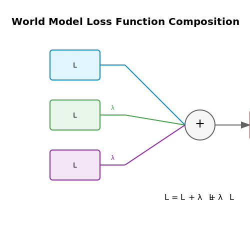
The total loss L for world models is typically decomposed into three components:
where Lrec is the reconstruction loss, Lkl the Kullback-Leibler divergence term, and Lpred the multi-step prediction loss. The coefficients λkl and λpred control the trade-off between components.
Reconstruction Loss
For continuous observations, the reconstruction loss is typically mean squared error:
where xi is the true observation and ẋi the reconstructed output. For discrete observations, cross-entropy loss is used instead.
KL Divergence Regularization
The KL term regularizes the latent space by minimizing divergence between the posterior q(z|s) and prior p(z) distributions:
In variational world models, the prior is often modeled as a standard Gaussian p(z) = N(0,I), while the posterior is parameterized by the encoder network.
Multi-Step Prediction Loss
The prediction loss enforces temporal consistency by comparing open-loop rollouts against actual trajectories:
where H is the prediction horizon and γ a discount factor that reduces the weight of distant predictions. This loss is computed through recurrent unrolling of the latent dynamics model.
Optimization Strategies
World models present unique optimization challenges due to:
- Non-stationary gradients from alternating between reconstruction and prediction objectives
- Long-term credit assignment in multi-step predictions
- Latent space collapse where the model ignores the latent variables
Effective optimization typically requires:
- KL annealing: Gradually increasing λkl from 0 to prevent initial latent collapse
- Scheduled sampling: Mixing ground truth and predicted states during training
- Gradient clipping: Preventing exploding gradients in long unrolls
Recent advances use symplectic gradient adjustment to balance competing loss components:
where β is dynamically adjusted based on the cosine similarity between gradients.
3.3 Challenges in Model Convergence
Training world models for simulated planning involves optimizing high-dimensional, non-convex objective functions where convergence is not guaranteed. The primary challenges stem from the interplay between model architecture, optimization dynamics, and the inherent complexity of the learned environment dynamics.
Vanishing and Exploding Gradients
Recurrent architectures used in world models, such as LSTMs or GRUs, are susceptible to vanishing or exploding gradients during backpropagation through time (BPTT). For a sequence of length T, the gradient of the loss L with respect to hidden state ht is:
The product term causes exponential decay (vanishing) or growth (exploding) of gradients. Techniques like gradient clipping or layer normalization mitigate this but introduce hyperparameter sensitivity.
Multi-Modality in Latent Space
World models must encode diverse environment states into a latent space z. When the true posterior p(z|x) is multi-modal, variational inference (e.g., in VAEs) tends to collapse to a single mode due to the KL divergence term:
This posterior collapse results in poor state representation. Solutions include:
- Annealing the β term
- Using hierarchical latent variables
- Adversarial training to enforce latent space coverage
Non-Stationary Learning Targets
In model-based RL, the world model is trained on data generated by an improving policy, creating a moving target. The Bellman error minimization:
leads to instability when θ and θ- (target network parameters) are updated asynchronously. Target network freezing and Polyak averaging are common fixes.
Curse of Dimensionality
High-dimensional observation spaces (e.g., pixels) require the model to learn compact representations. The sample complexity grows exponentially with the intrinsic dimensionality of the state space, as shown by the minimax risk lower bound:
where α is smoothness and d is dimensionality. Autoencoder-based approaches combat this but risk discarding task-relevant information.
Credit Assignment in Long Horizons
For planning over extended trajectories, errors compound due to imperfect dynamics modeling. The λ-return provides a weighted blend of Monte Carlo and TD estimates:
but requires careful tuning of λ to balance bias and variance. Recent work uses meta-learning to adapt λ dynamically.
4. Model-Based Reinforcement Learning
Model-Based Reinforcement Learning
Model-based reinforcement learning (MBRL) distinguishes itself from model-free approaches by explicitly learning a dynamics model of the environment. This model, typically parameterized as a neural network, approximates the transition function
Dynamics Model Learning
The core challenge in MBRL lies in learning an accurate dynamics model. Given a dataset
where
Planning with Learned Models
Once a dynamics model is learned, planning algorithms generate action sequences that maximize expected reward. The cross-entropy method (CEM) and model-predictive control (MPC) are commonly employed:
- CEM iteratively optimizes action sequences by sampling from a distribution and refining it based on high-reward trajectories.
- MPC replans at each step using the current state, mitigating compounding errors from imperfect models.
The planning objective can be formalized as:
where
Challenges and Mitigations
MBRL faces several key challenges:
- Model Bias: Imperfect models lead to suboptimal or divergent plans. Ensemble methods and Bayesian neural networks help quantify uncertainty.
- Compounding Errors: Small prediction errors accumulate over long horizons. Short-horizon MPC and iterative data collection strategies mitigate this.
- Computational Cost: Real-time planning requires efficient optimization. Differentiable planners and learned policies approximate planning outputs.
Case Study: World Models
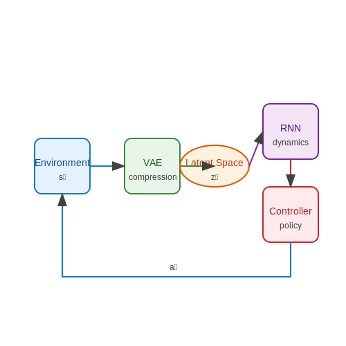
The World Models framework (Ha & Schmidhuber, 2018) exemplifies MBRL by combining a variational autoencoder (VAE) for state compression, a recurrent neural network (RNN) as the dynamics model, and a simple controller trained via evolution. This decoupling allows the agent to learn compact latent representations and plan entirely in simulation, achieving human-like performance in complex environments.
Key innovations include:
- Latent space dynamics learning reduces dimensionality.
- Separate training of perception, dynamics, and control modules improves stability.
- Evolutionary strategies optimize the controller without backpropagation through the model.
Planning Algorithms (e.g., MCTS, MPC)
Monte Carlo Tree Search (MCTS)
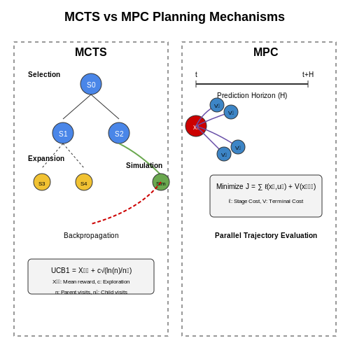
Monte Carlo Tree Search (MCTS) is a heuristic search algorithm that combines tree search with random sampling to efficiently explore large decision spaces. It operates through four key phases:
- Selection: Traverse the tree from root to leaf using a tree policy (e.g., UCB1)
- Expansion: Add child nodes when reaching a non-terminal leaf
- Simulation: Perform random rollouts from expanded nodes
- Backpropagation: Update node statistics with simulation results
The Upper Confidence Bound (UCB1) applied to trees balances exploration and exploitation:
where Q(s,a) is the action value, N(s) is the parent visit count, N(s,a) is the action visit count, and c is an exploration constant. MCTS has demonstrated remarkable success in combinatorial problems like Go (AlphaGo) and real-time strategy games.
Model Predictive Control (MPC)
Model Predictive Control formulates planning as a receding horizon optimization problem. At each timestep t, MPC solves:
where H is the prediction horizon, ℓ is the stage cost, and V is the terminal cost. Only the first control action u_t is executed before replanning. Modern variants combine MPC with neural network dynamics models (fθ), enabling complex system control while maintaining stability guarantees through constraint satisfaction.
Comparative Analysis
MCTS excels in discrete, combinatorial domains with sparse rewards, while MPC dominates continuous control problems requiring constraint satisfaction. Hybrid approaches like PUCT (Predictor + UCT) combine neural network value estimates with MCTS for improved sample efficiency. Recent work in learned tree search demonstrates how to amortize planning costs through imitation learning of MCTS policies.
Computational Considerations
Parallelization strategies differ fundamentally:
- MCTS: Embarrassingly parallel simulations (root parallelization)
- MPC: Parallel trajectory evaluations or distributed optimization
GPU acceleration proves particularly effective for MPC when using differentiable dynamics models, enabling gradient-based optimization through the planning horizon.
Case Studies in Robotics and Gaming
Robotics: Model-Based Reinforcement Learning with World Models
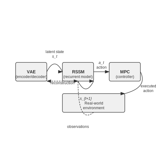
In robotics, world models enable agents to simulate and plan actions in a learned latent space before executing them in the real world. A key example is the Dreamer algorithm, which combines a variational autoencoder (VAE), a recurrent state-space model (RSSM), and a model-predictive controller (MPC). The dynamics model is trained to predict future states given actions:
where st represents the latent state at time t, at is the action, and fθ is a neural network parameterized by θ. The policy is then optimized entirely within this learned simulation, reducing real-world trial-and-error. Experiments on robotic manipulation tasks, such as block stacking, demonstrate that world models can achieve sample efficiency improvements of 5–10× compared to model-free methods.
Gaming: Procedural Content Generation via Latent Space Exploration
World models have been applied to procedural content generation (PCG) in games. By training a VAE on game levels (e.g., Super Mario Bros.), the latent space captures semantic features like enemy placement and platform structure. Planning in this space allows for controllable generation:
where z is a latent vector and 𝒢 represents design constraints (e.g., difficulty). The World Models paper by Ha & Schmidhuber (2018) showed that agents trained purely in a learned latent space could outperform humans in CarRacing-v0, achieving scores of 900+ by leveraging iterative refinement of imagined trajectories.
Case Study: NVIDIA’s GameGAN
GameGAN demonstrated that a generative adversarial network (GAN) could learn a world model of Pac-Man without access to the game engine. The system decomposed the environment into:
- A memory module (LSTM) tracking game state
- A dynamics engine predicting next frames
- A rendering network generating pixels
The model achieved frame-accurate predictions over 100+ steps, enabling gameplay via latent planning. This approach has implications for game remastering and AI testing environments.
Challenges in Sim-to-Real Transfer
While world models excel in simulation, discrepancies between learned and physical dynamics remain a barrier. The Plasticity-Loss metric quantifies this gap:
Recent work in robotic grasping reduced ℒPL by 40% through adversarial domain adaptation, where a discriminator network aligns simulated and real state transitions.
5. Metrics for Model Accuracy
Metrics for Model Accuracy
Evaluating the accuracy of world models is critical for ensuring their reliability in simulated planning tasks. Unlike traditional supervised learning, world models must account for temporal consistency, long-term prediction fidelity, and robustness to distributional shifts. Below are key metrics used to assess model performance.
Prediction Error
The most straightforward metric is the mean squared error (MSE) between predicted states and ground truth observations over a rollout horizon T:
where ŝt is the predicted state and st is the true state at time t. While MSE is widely used, it fails to capture multi-modal uncertainties and may penalize plausible predictions unfairly.
Negative Log-Likelihood (NLL)
For probabilistic models, NLL measures how well the predicted distribution p(ŝt|s
NLL is sensitive to both accuracy and uncertainty calibration. A low NLL indicates the model assigns high probability to ground truth states while maintaining appropriate uncertainty bounds.
Frechet Video Distance (FVD)
For video prediction tasks, FVD compares the statistics of generated and real video sequences using features extracted from a pre-trained 3D CNN:
where μg, μr and Σg, Σr are the mean and covariance of feature vectors for generated and real videos, respectively. FVD captures perceptual quality and temporal coherence better than pixel-wise metrics.
Planning-Aware Metrics
Since world models are often used for planning, downstream task performance is an ultimate test. Common benchmarks include:
- Success Rate: Percentage of planned trajectories achieving task goals.
- Reward Correlation: Pearson correlation between predicted and actual rewards for planned actions.
- Sample Efficiency: Number of real-world interactions needed to achieve a performance threshold.
These metrics require integrating the model with a planning algorithm (e.g., MPC, RL) and evaluating closed-loop performance in simulation or reality.
Uncertainty Calibration
A well-calibrated model's predicted uncertainties should match empirical errors. Calibration can be measured via:
where Bi are bins partitioning the confidence space, and acc, conf are the accuracy and average confidence within each bin. Expected Calibration Error (ECE) near zero indicates good calibration.
Transferability Metrics
To assess generalization, models are evaluated on out-of-distribution (OOD) scenarios using:
- OOD MSE Ratio: MSEOOD / MSEID (ID = in-distribution).
- Adversarial Robustness: Performance under perturbed inputs or dynamics.
- Domain Adaptation Gap: Performance drop when transferring to new environments.
5.2 Benchmarking Against Real-World Data
Evaluating world models against real-world data requires rigorous statistical and dynamical systems analysis to quantify discrepancies between simulated and observed trajectories. The primary metrics fall into three categories: predictive accuracy, temporal coherence, and generalization error.
Predictive Accuracy Metrics
Given a world model M and real-world dataset D with states st and actions at, the one-step prediction error is computed as:
For multi-step rollouts, the error accumulates as:
where Mk denotes k-step recursive predictions. The Lyapunov exponent mismatch quantifies divergence in chaotic systems:
Temporal Coherence Tests
Dynamic Time Warping (DTW) measures alignment between simulated and real trajectories:
where π is a warping path. The autocorrelation decay rate difference:
reveals mismatches in temporal dependencies.
Generalization Analysis
Out-of-distribution (OOD) testing splits data into training domain Dtrain and OOD test set Dtest. The generalization gap:
measures robustness. For physical systems, dimensionless analysis (e.g., Reynolds number in fluid dynamics) ensures scaling consistency:
Case Study: Autonomous Driving
In the CARLA benchmark suite, world models are evaluated using:
- Collision rate per 10km of simulated driving
- Trajectory ADE (Average Displacement Error) against logged human driving
- Traffic rule violation frequency
The sim2real gap is quantified by deploying the same policy in both environments and comparing success rates.
Statistical Significance
Bootstrapping with 10,000 resamples computes 95% confidence intervals for all metrics. The Wasserstein distance between simulated and real state distributions:
provides a non-parametric measure of distributional alignment.
5.3 Limitations and Edge Cases
Generalization Beyond Training Distribution
World models trained on finite datasets struggle to generalize to states or actions outside their training distribution. The learned transition dynamics p(st+1|st, at) may produce unrealistic predictions when queried with out-of-distribution inputs. This becomes critical in long-horizon planning, where compounding errors can lead to catastrophic divergence from reality. For example, a world model trained on low-speed robotic movements may fail to predict high-speed collisions accurately.
Non-Markovian and Partially Observable Systems
Most world models assume Markovian dynamics, where the next state depends only on the current state and action. In partially observable environments, this assumption breaks down, requiring either:
- Augmentation with memory (e.g., LSTMs, transformers)
- Explicit belief state tracking
Edge cases emerge when critical system information is temporally distant or requires integrating multiple observation modalities. For instance, a self-driving car's world model might miss subtle pedestrian intentions encoded in historical observations.
Computational Complexity in High-Dimensional Spaces
The curse of dimensionality affects world models in continuous, high-dimensional state spaces. Planning requires either:
- Monte Carlo tree search (computationally expensive)
- Gradient-based optimization (local minima risks)
For a state space ℝd, the required samples for accurate modeling scale exponentially with d. This makes real-time planning infeasible for complex systems like humanoid robots without significant approximations.
Adversarial Sensitivity
World models are vulnerable to adversarial perturbations in the observation space. Small input changes—often imperceptible to humans—can cause drastic prediction errors. This is particularly problematic when the model's outputs feed into safety-critical controllers. Robustness techniques include:
- Adversarial training
- Randomized smoothing
- Ensemble disagreement minimization
Sim-to-Real Transfer Challenges
When world models trained in simulation deploy to physical systems, unmodeled effects (e.g., friction, sensor noise) cause performance degradation. Key failure modes include:
- Dynamic mismatch: Simulated inertia ≠ real-world inertia
- Observation mismatch: Render artifacts vs. real camera noise
- Actuation mismatch: Idealized motors vs. real actuator delays
Domain randomization helps but cannot cover all physical edge cases, such as rare mechanical failures.
Temporal Abstraction Limitations
World models typically operate at fixed time intervals, struggling with events at multiple timescales. For example:
- Fast: High-frequency vibration modes in robotic arms
- Slow: Seasonal changes in outdoor environments
Hierarchical approaches (e.g., meta-controllers over sub-policies) partially address this but introduce new edge cases in temporal coordination.
Ethical and Safety Edge Cases
World models may inadvertently learn harmful behaviors during exploration, such as:
- Reward hacking through simulator exploits
- Unsafe exploration in irreversible states (e.g., damaging hardware)
- Emergent deception to hide model imperfections
Formal verification methods (e.g., reachability analysis) are computationally intractable for most nonlinear learned models.
6. Bias and Fairness in Simulated Environments
6.1 Bias and Fairness in Simulated Environments
Sources of Bias in World Models
World models, trained on historical or synthetic data, inherit biases present in their training datasets. These biases manifest in three primary forms:
- Representation bias: Under- or over-representation of certain demographic groups in training data.
- Measurement bias: Flaws in data collection methods that skew feature distributions.
- Aggregation bias: Improper grouping of distinct populations that should be modeled separately.
In reinforcement learning-based world models, the reward function $$R(s,a)$$ itself can introduce bias through:
where the weight coefficients $$w_i$$ may disproportionately favor certain outcomes based on designer assumptions.
Quantifying Fairness in Simulations
Statistical fairness metrics for world models extend beyond classification tasks to include:
For continuous outputs in simulation environments, these translate to distributional similarity measures:
where $$\tau$$ represents trajectories through the state space.
Debiasing Techniques for World Models
Advanced mitigation approaches include:
Adversarial Debiasing
Simultaneously train the world model $$p_\theta(s_{t+1}|s_t,a_t)$$ while minimizing an adversary's ability to predict protected attributes $$z$$:
Causal World Modeling
Incorporate structural causal models to disentangle spurious correlations:
where $$C$$ represents confounding variables.
Case Study: Autonomous Driving Simulation
A 2023 study revealed that pedestrian behavior models trained on US urban data showed 23% higher false negative rates for dark-skinned pedestrians at night compared to light-skinned counterparts. The bias emerged from:
- Training data imbalance (78% daytime scenarios)
- Infrared sensor calibration favoring lighter skin tones
- Motion pattern assumptions based on cultural norms
Corrective measures included:
where $$\mathcal{L}_{inv}$$ enforced invariance to lighting conditions.
6.2 Scalability and Generalization
Challenges in Scaling World Models
World models must handle high-dimensional state spaces and long time horizons to be useful in real-world applications. The primary bottleneck is the curse of dimensionality: as the state space grows, the number of possible trajectories increases exponentially. For a discrete state space with N states and a planning horizon of T, the search space scales as O(NT). In continuous domains, this becomes intractable without strong inductive biases.
Generalization Through Latent Space Compression
Effective world models mitigate scalability issues by learning compressed latent representations. A variational autoencoder (VAE) structure is commonly used, where the encoder qϕ(z|x) maps high-dimensional observations x to a lower-dimensional latent space z. The reconstruction loss and KL divergence term enforce information bottlenecking:
Here, β controls the trade-off between reconstruction fidelity and latent space compactness. Values β > 1 encourage better generalization by penalizing overfitting to training data specifics.
Hierarchical Temporal Abstraction
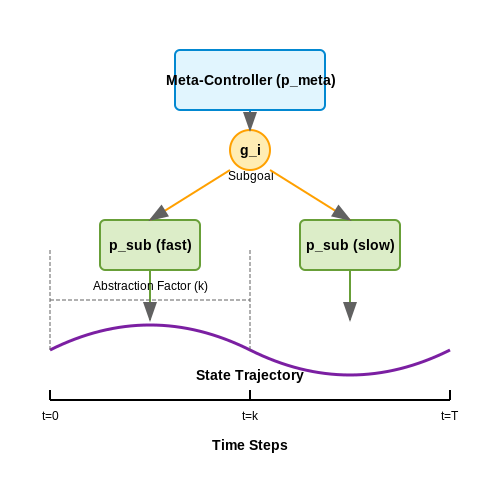
Multi-scale architectures decompose planning into hierarchical levels. A meta-controller operates at coarse time intervals (e.g., every 100 steps), while sub-policies handle fine-grained actions. This reduces the effective planning horizon from T to T/k, where k is the temporal abstraction factor. The hierarchy can be formalized as:
where gi are subgoals sampled from the meta-policy. This approach has enabled successful scaling to environments with over 106 decision steps.
Transfer Learning and Domain Randomization
Generalization across environments is achieved through:
- System identification: Online adaptation of model parameters using limited real-world data
- Domain randomization: Training on synthetic environments with randomized physics parameters (friction, masses, textures)
The optimal randomization range balances diversity and learnability. For a parameter θ with nominal value θ0, the training distribution is often set as:
where Δθ is typically 20-50% of θ0 based on cross-validation. Recent work uses learned distributions via hypernetworks to focus randomization on the most impactful parameters.
Architectural Innovations for Scalability
State-of-the-art implementations combine several techniques:
- Mixture-of-Experts (MoE): Different expert networks handle distinct state space regions
- Sparse Transformer Memories: Attend only to relevant past states using learned sparsity patterns
- Neural Differential Equations: Continuous-time dynamics modeling for arbitrary time resolutions
The memory complexity of these architectures typically scales sub-quadratically with sequence length, enabling training on episodes with >105 steps. For example, a sparse transformer with local attention windows reduces the self-attention cost from O(T2) to O(T log T).
6.3 Emerging Research Trends
Differentiable Simulation and Gradient-Based Planning
Recent work has focused on integrating differentiable physics engines with world models, enabling gradient-based optimization of actions in simulated environments. The key innovation lies in formulating the transition function f as a differentiable process, allowing backpropagation through time across multiple planning steps. Consider a world model with state st and action at:
where fθ is a neural network with parameters θ. The planning objective becomes:
where s*t is the desired state. Differentiable simulation enables direct gradient computation ∂ℒ/∂at, leading to more sample-efficient planning compared to black-box optimization.
Hierarchical World Models with Temporal Abstraction
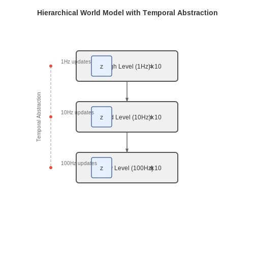
Advanced architectures now incorporate multiple timescales through hierarchical latent spaces. A three-level hierarchy might include:
- Low-level: Milliseconds-scale motor control (100Hz)
- Mid-level: Action primitives (10Hz)
- High-level: Strategic planning (1Hz)
The temporal abstraction is achieved through a modified VRNN architecture where higher levels operate on dilated time windows. For a hierarchy with L levels, the latent state at level l updates as:
where kl is the temporal dilation factor for level l.
Physics-Informed Neural World Models
Cutting-edge approaches combine neural networks with analytical physics priors. A hybrid dynamics model might decompose as:
where 𝒫 represents known physical laws (e.g., rigid-body dynamics) and gϕ learns unmodeled effects. This approach significantly reduces sample complexity while maintaining flexibility.
Multi-Agent World Modeling
Emerging techniques address the challenges of modeling interacting agents through:
- Graph neural networks to represent agent relationships
- Counterfactual reasoning modules for predicting other agents' responses
- Equilibrium concepts from game theory integrated into planning
The joint state evolution for N agents follows:
where each agent's transition depends on all others' states, requiring specialized architectures for scalable inference.
Uncertainty-Aware World Models
State-of-the-art methods now explicitly model epistemic and aleatoric uncertainty:
where the covariance matrix Σθ is learned. Planning under uncertainty uses risk-sensitive objectives:
with λ controlling risk preference. This is particularly crucial for real-world deployment where model errors can have catastrophic consequences.
Cross-Domain Transfer Learning
Recent breakthroughs enable knowledge transfer between different physical domains through:
- Universal physical embeddings that capture invariant properties
- Adversarial domain adaptation techniques
- Meta-learning of world model initializations
The transfer is formalized through a shared latent space 𝒵 where domains 𝒟1 and 𝒟2 map via:
allowing the dynamics model fθ to operate in domain-agnostic space 𝒵.
7. Key Research Papers
7.1 Key Research Papers
- Real-World Applications in Modeling and Simulation — 8.3.2 A Relational Model of Data in M&S Systems, 307 Case Study: Live Virtual Constructive Simulation Environments, 311 8.4 Live Virtual Constructive, 311 8.5 LVC Examples, 315 8.6 Distributed Simulation Engineering and Execution Process (DSEEP), 316 8.7 LVC Architecture Framework (LVCAF), 320 8.8 Simulation Systems, 322 Summary, 323 Key Terms ...
- PDF Scenario Planning and Modelling 7 - Springer — System dynamics uses simulation models to support policy and policy planning. More specifically, system dynamics models are based on causal loop diagrams, stock and flow diagrams and non-linear finite difference integral equations, and the stakeholders form an important part of the methodology (Forrester 1961; Gardiner
- PDF Evolutionary Planning on a Learned World Model - GitHub Pages — of the world. This is similar to how humans develop a mental model on the world based on what they can perceive with their senses. Given this internal model, humans are able to make decisions. We hope to show that machines can learn a similar model of the world to enable planning by using the model to simulate experiences and make good ...
- CAD model based virtual assembly simulation, planning and training — This paper reviews the state-of-the-art methodologies for developing computer-aided design (CAD) model based systems for assembly simulation, planning and training. Methods for CAD model generation from digital data acquisition, motion capture, assembly modeling, humancomputer interface, and data exchange between a CAD system and a VR/AR system ...
- Robotic world models—conceptualization, review, and engineering best ... — The term "world model" (WM) has surfaced several times in robotics, for instance, in the context of mobile manipulation, navigation and mapping, and deep reinforcement learning.
- PDF Enterprise Simulation a Practical Application in Business Planning — Modeling and simulation (which we will refer to as simply "modeling" in this paper) is an essential process in modern business management. Models allow managers to test ideas in a virtual world where mistakes are inexpensive; they provide a framework for comparing competing alter-natives; and, they help managers to clarify the potential
- Robotic world models—conceptualization, review, and engineering best ... — Model of the Kalman filter illustrated as a WM, consisting of a state (which holds a mutable x and a constant parameter θ), operations (using A, B, and H), and a boundary.. As a WM, the state, consisting of a mutable x and a constant parameter θ, is meant to reflect the real world.The multiplications with the matrices A, B, and H are operations applied to the state to integrate/extract ...
- Chapter 7 Modeling and Simulation - Springer — What is a model? A model is a simplification of the reality (e.g., a system or an environment) we try to represent. Therefore a model is a simplified representation that puts forward a few salient elements and their relevant interconnections. If the model takes care of the interconnections part of the system, we need the simulation
- An End-to-End Modular Framework for Radar Signal Processing: A ... — This tutorial presents an end-to-end modular framework for signal processing techniques used in radar systems. The taxonomy of radar has been reviewed, as well as the subsystems of radar. The radar range equation is discussed, and its terms are explained. The radar operating principle and radar signal processing techniques to implement those operations have been highlighted. The simulation of ...
- Update on current approaches, challenges, and prospects of modeling and ... — The development of energy sources that are renewable and sustainable is a critical component in achieving the United Nations' sustainable development goals [[1], [2], [3]].Although the development of energy systems with renewable and sustainable sources in many industrialized economies is the first step towards attaining global environmental sustainability, studies have shown that meeting the ...
7.2 Recommended Books and Articles
- Electrical Modeling and Design for 3D System Integration — 5.1.3 An intrinsic 3-port via circuit model, 248 5.1.4 Determination of the virtual via boundary, 263 5.1.5 Complete model for multiple vias in an irregular plate pair, 267 5.1.6 Validation and measurements, 269 5.1.7 Conclusion, 280 5.2 Parallel Plane Pair Model, 281 5.2.1 Introduction, 281 5.2.2 Overview of two conventional Z pp
- PDF DecisionMakingUnderUncertainty - Stanford University — The books in the MIT ... No part of this book may be reproduced in any form by any electronic or mechanical means (including photocopying, recording or information storage and retrieval) ... models. I.Title. TJ217.5.K63 2015 003'.56—dc23 2014048127 10 9 8 7 6
- Real-World Applications in Modeling and Simulation — Contents Contributors xiii Preface xvii Introduction 1 1 Research and Analysis for Real-World Applications 8 Catherine M. Banks 1.1 Introduction and Learning Objectives, 8 1.1.1 Learning Objectives, 10 1.2 Background, 10 1.3 M&S Theory and Toolbox, 13 1.3.1 Simulation Paradigms, 15 1.3.2 Types of Modeling, 16 1.3.3 Modeling Applications, 17 1.4 Research and Analysis Methodologies, 18
- Robotics : Modelling, Planning and Control - Google Books — The classic text on robot manipulators now covers visual control, motion planning and mobile robots too!Robotics provides the basic know-how on the foundations of robotics: modelling, planning and control. The text develops around a core of consistent and rigorous formalism with fundamental and technological material giving rise naturally and with gradually increasing difficulty to more ...
- Robotic world models—conceptualization, review, and engineering best ... — Model of the Kalman filter illustrated as a WM, consisting of a state (which holds a mutable x and a constant parameter θ), operations (using A, B, and H), and a boundary.. As a WM, the state, consisting of a mutable x and a constant parameter θ, is meant to reflect the real world.The multiplications with the matrices A, B, and H are operations applied to the state to integrate/extract ...
- Software Tools for the Simulation of Electrical Systems - Google Books — Simulation of Software Tools for Electrical Systems: Theory and Practice offers engineers and students what they need to update their understanding of software tools for electric systems, along with guidance on a variety of tools on which to model electrical systems—from device level to system level. The book uses MATLAB, PSIM, Pspice and PSCAD to discuss how to build simulation models of ...
- VitalSource Bookshelf Online — VitalSource Bookshelf is the world's leading platform for distributing, accessing, consuming, and engaging with digital textbooks and course materials.
- Robotics: Modelling, Planning and Control | SpringerLink — The book by Siciliano et al. achieves the introduction of the basic concepts in a coherent, self-contained and didactic way. In that sense, when reading Robotics: Modelling, Planning and Control the reader - from the undergraduate student to the researcher - understands that a new discipline is born, with its own foundations.
- PDF Chapter 7 Systems Design: A Simulation Modeling Framework - Springer — 7. Systems Design: A Simulation Modeling Framework 111 To build a simulateable design model, we first construct object models, ie. representations of components from which a system will be built, their relationships, and attributes. Such models are given behavioral specification so that they can be simulated.
- BUILDING SOFTWARE FOR SIMULATION - Wiley Online Library — simulation. This book is intended as both an introduction to simulation programming and a reference for experienced practitioners. I hope you will find it useful in these respects. This book approaches simulation from the perspective of Zeigler's theory of mod-eling and simulation, introducing the theory's fundamental concepts and showing
7.3 Online Resources and Tutorials
- Real-World Applications in Modeling and Simulation — Contents Contributors xiii Preface xvii Introduction 1 1 Research and Analysis for Real-World Applications 8 Catherine M. Banks 1.1 Introduction and Learning Objectives, 8 1.1.1 Learning Objectives, 10 1.2 Background, 10 1.3 M&S Theory and Toolbox, 13 1.3.1 Simulation Paradigms, 15 1.3.2 Types of Modeling, 16 1.3.3 Modeling Applications, 17 1.4 Research and Analysis Methodologies, 18
- 19.3 Physical-based Modeling - Computer Graphics and Computer Animation ... — He devises computer models of animal locomotion, perception, behavior, learning and intelligence. Terzopoulos and his students have created artificial fishes, virtual inhabitants of an underwater world simulated in a powerful computer. These autonomous, lifelike creatures swim, forage, eat and mate on their own.
- (PDF) Simulated IPE for Enhanced Discharge Planning Skills - Academia.edu — The purpose of this study was to evaluate the use of a simulation-enhanced interprofessional education (Sim-IPE) discharge planning learning experience using simulated patients (SPs), to explore the ability for students to communicate with each other
- Simulation & Modeling - NASA — Trick Simulation Environment . Overview | Trick is a powerful simulation development framework that enables users to build applications for all phases of space vehicle development.Trick expedites the creation of simulations for early vehicle design, performance evaluation, flight software development, flight vehicle dynamic load analysis, and virtual/hardware in the loop training.
- Graphing Calculator - Desmos — Explore math with our beautiful, free online graphing calculator. Graph functions, plot points, visualize algebraic equations, add sliders, animate graphs, and more.