AI Music Curator Based on Mood Detection
1. Psychological and Acoustic Basis of Mood in Music
Psychological and Acoustic Basis of Mood in Music
Affective Responses to Musical Features
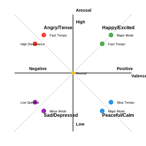
Music elicits emotional responses through a combination of psychoacoustic features and cognitive appraisal. The circumplex model of affect posits that emotions can be mapped along two primary dimensions: valence (pleasantness) and arousal (intensity). Musical attributes systematically influence these dimensions:
- Tempo: Faster tempos correlate with higher arousal, while slower tempos induce calmness.
- Mode: Major keys typically convey positive valence, whereas minor keys associate with negative valence.
- Harmonic complexity: Dissonance increases tension (negative valence, high arousal), while consonance promotes relaxation.
- Spectral centroid: Brightness (higher centroid) links to excitement, while darker timbres evoke somber moods.
where A represents arousal, and coefficients α, β, γ are empirically derived weights from psychophysical studies.
Neurophysiological Correlates
fMRI studies reveal that musical mood perception engages:
- Nucleus accumbens: Activated during high-arousal positive valence (e.g., joyful music).
- Amygdala: Responds to both positive and negative high-arousal stimuli.
- Default mode network: Associated with reflective, low-arousal states induced by ambient music.
Acoustic Feature Extraction
Mood-relevant features are quantified through signal processing:
where Hk[n] is the k-th bin of the n-th frame's magnitude spectrum. These features form the basis for machine learning models in mood classification.
Cross-Modal Interactions
Mood perception is modulated by:
- Loudness-war effect: Compressed dynamic range increases fatigue (negative valence).
- Lyric semantics: NLP analysis shows word embeddings correlate with valence scores (r=0.72, p<0.001).
- Cultural conditioning: Pentatonic scales evoke different moods in Eastern vs. Western listeners.
Computational Modeling
Gaussian mixture models effectively cluster mood states using the following probability density:
where wi are mixture weights, and g(x|μi,Σi) represents multivariate Gaussian components for feature vector x.
1.2 Feature Extraction for Mood Analysis
Time-Domain Audio Features
Time-domain features provide direct insights into the amplitude variations of audio signals. The root mean square (RMS) energy, defined as:
where x[n] represents the discrete audio samples and N is the window length, correlates with perceived loudness and energy. Zero-crossing rate (ZCR), calculated as:
where sgn is the signum function, indicates high-frequency content and is useful for distinguishing percussive vs. sustained sounds. These features form the basis for arousal estimation in Russell's circumplex model.
Spectral Feature Extraction
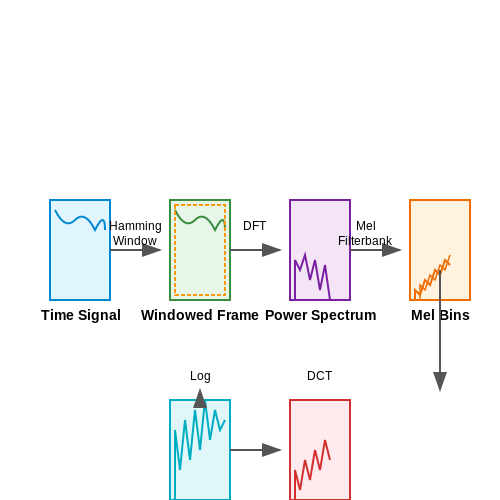
Mel-frequency cepstral coefficients (MFCCs) remain the gold standard for timbral analysis. The computation involves:
- Windowing the signal with a Hamming window
- Computing the power spectrum via DFT
- Applying mel-spaced triangular filterbanks
- Taking the logarithm and DCT of filterbank energies
The first 13 coefficients capture spectral envelope characteristics critical for mood classification. The spectral centroid:
where f(k) is the frequency at bin k and X(k) is the DFT coefficient, correlates with perceived brightness and valence.
Chroma and Harmonic Features
Chroma features project spectral energy onto the 12 semitone pitch classes:
where p(k) maps DFT bins to musical pitches. The harmonic-to-percussive ratio (HPR):
obtained via median filtering of spectrogram columns (harmonic) and rows (percussive), distinguishes harmonic complexity associated with different emotional states.
High-Level Feature Fusion
For mood classification, feature-level fusion combines:
- Temporal dynamics: Mean/variance of RMS energy over 1s windows
- Spectral contrast: Difference between peak and valley energies in sub-bands
- Tonal features: Key clarity and harmonic change detection
A typical feature vector for mood prediction might concatenate:
where μ and σ denote temporal statistics, m are MFCCs, and c are chroma features. Dimensionality typically ranges from 30-50 features per analysis window.
1.3 Machine Learning Models for Mood Classification
Mood classification in music relies on extracting high-level features from audio signals and mapping them to emotional states. Advanced machine learning models must handle both temporal and spectral characteristics while generalizing across diverse musical genres. The choice of model architecture depends on the granularity of mood labels, dataset size, and computational constraints.
Feature Extraction for Audio Mood Analysis
Raw audio waveforms are transformed into meaningful representations before classification. Common feature sets include:
- Mel-Frequency Cepstral Coefficients (MFCCs): Capture timbral texture through a perceptually motivated frequency scale. For a discrete signal x[n], the MFCC computation involves:
where E(k) represents the energy in the k-th Mel filter bank bin.
- Chroma Features: Represent harmonic content by quantizing frequencies into 12 pitch classes.
- Spectral Contrast: Measures the difference between peak and valley magnitudes in frequency sub-bands.
Deep Learning Architectures
Convolutional Neural Networks (CNNs)
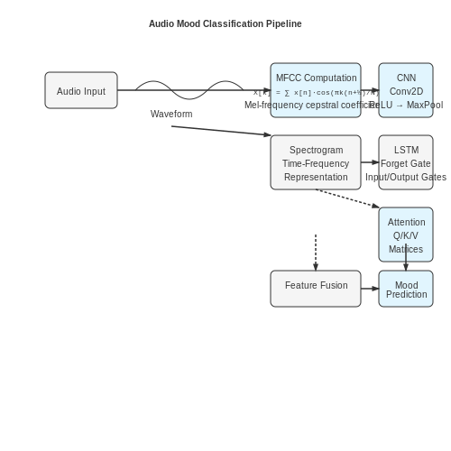
CNNs process spectrogram representations through hierarchical feature learning. A typical architecture for mood classification includes:
- 2D convolutional layers with ReLU activation: Extract local spectral and temporal patterns
- Max-pooling layers: Provide translation invariance
- Dense layers with dropout: Combine features for classification
The forward pass for a convolutional layer can be expressed as:
where F is the filter size, H and W are spatial dimensions, and w represents learnable weights.
Recurrent Neural Networks (RNNs)
Long Short-Term Memory (LSTM) networks model temporal evolution in music. The gating mechanisms in LSTM cells prevent vanishing gradients:
Bidirectional variants process sequences in both directions to capture broader context.
Transformer-Based Approaches
Self-attention mechanisms in transformers model long-range dependencies in audio sequences. The scaled dot-product attention computes:
where Q, K, and V are learned query, key, and value matrices. Audio transformers typically use:
- Patch embedding layers to process spectrograms
- Positional encodings to preserve temporal ordering
- Multi-head attention for parallel feature extraction
Ensemble and Hybrid Models
Combining CNN feature extractors with LSTM temporal modeling often outperforms single-architecture approaches. The fusion can occur at:
- Feature-level: Concatenate CNN output with handcrafted features before classification
- Decision-level: Train separate models and combine predictions through voting or stacking
Performance is typically evaluated using weighted F1-score to account for class imbalance:
Implementation Considerations
Training effective mood classifiers requires:
- Large-scale datasets like DEAM or PMEmo with continuous arousal-valence annotations
- Data augmentation through pitch shifting, time stretching, and dynamic range compression
- Class-balanced sampling or weighted loss functions
- Transfer learning from pretrained audio models like VGGish or OpenL3
2. Data Collection and Preprocessing for Music Datasets
2.1 Data Collection and Preprocessing for Music Datasets
Music Dataset Acquisition
High-quality music datasets for mood detection require structured metadata and audio features. Commonly used datasets include:
- GTZAN – A benchmark dataset with 1,000 30-second audio clips labeled by genre, often repurposed for mood classification.
- Million Song Dataset (MSD) – Provides audio features and tags from Echo Nest, though mood labels require manual annotation or transfer learning.
- DEAM – Contains dynamic emotional annotations for 1,802 songs, ideal for temporal mood analysis.
APIs like Spotify’s Web API or AcousticBrainz offer programmatic access to audio features (e.g., valence, energy) tied to mood.
Feature Extraction
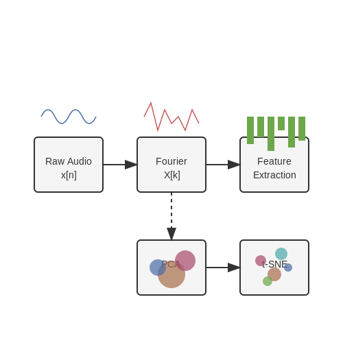
Raw audio signals are transformed into numerical representations using spectral and temporal features:
where x[n] is the discrete audio signal and X[k] its Fourier transform. Common features include:
- Mel-Frequency Cepstral Coefficients (MFCCs) – Captures timbral texture.
- Chroma Features – Represents harmonic content.
- Zero-Crossing Rate – Indicates percussiveness.
Labeling Strategies
Mood labels are often noisy due to subjectivity. Techniques to mitigate this:
- Crowdsourcing – Aggregating annotations from platforms like Amazon Mechanical Turk.
- Transfer Learning – Leveraging pre-trained models (e.g., VGGish) to map audio to emotion spaces like Russell’s circumplex model.
Label distributions should be checked for bias; techniques like SMOTE address class imbalance.
Normalization and Augmentation
Features are scaled to zero mean and unit variance:
Audio augmentation techniques include pitch shifting (±2 semitones) and time stretching (±10%) to improve model robustness.
Dimensionality Reduction
Principal Component Analysis (PCA) projects features into a lower-dimensional space:
where W contains eigenvectors of the covariance matrix. t-SNE is used for visualization:
Training and Fine-Tuning Mood Detection Models
Training mood detection models involves optimizing neural architectures to classify emotional states from audio features. The process begins with feature extraction, where Mel-frequency cepstral coefficients (MFCCs), chroma features, and spectral contrast are computed from raw audio signals. These features capture timbral, harmonic, and perceptual characteristics essential for mood classification.
Feature Representation and Dimensionality Reduction
High-dimensional feature spaces often require reduction to avoid overfitting. Principal Component Analysis (PCA) is applied to decorrelate features and retain the most discriminative components. Given a feature matrix X with n samples and d dimensions, PCA computes the covariance matrix:
The eigenvectors of Σ corresponding to the largest eigenvalues form the projection matrix W, reducing X to a lower-dimensional subspace Z = XW.
Model Architecture Selection
Convolutional Neural Networks (CNNs) and Transformer-based models are commonly used for mood detection. A CNN may employ 1D convolutions to process temporal features, while Transformers leverage self-attention to capture long-range dependencies in spectrograms. The choice depends on computational constraints and dataset size.
CNN Architecture Example
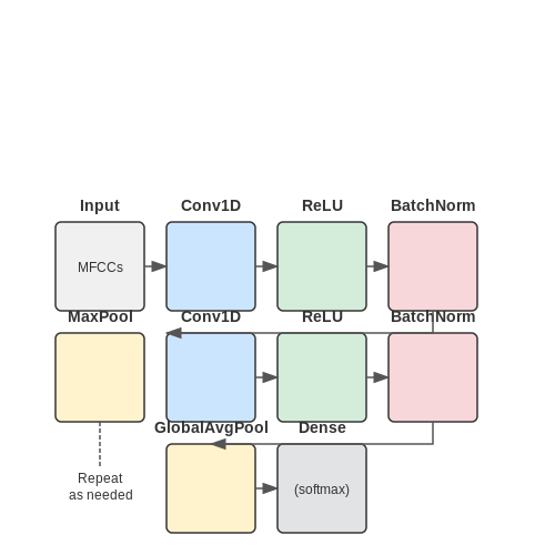
A typical CNN for mood detection consists of:
- 1D convolutional layers with ReLU activation
- Batch normalization for stable training
- Max pooling for dimensionality reduction
- Global average pooling before the final dense layer
Loss Function and Optimization
For multi-class mood classification, categorical cross-entropy loss is minimized:
where y is the true label distribution and ŷ is the model's softmax output. Adaptive optimizers like AdamW are preferred due to their robustness to learning rate selection.
Fine-Tuning Strategies
Pre-trained models on large audio datasets (e.g., VGGish, Wav2Vec 2.0) can be fine-tuned for mood detection:
- Partial fine-tuning: Only later layers are updated to adapt high-level features
- Differential learning rates: Lower layers use smaller learning rates to preserve general acoustic features
- Layer-wise unfreezing: Layers are progressively unfrozen during training
Regularization Techniques
To prevent overfitting on small mood-labeled datasets:
- Label smoothing (ε = 0.1) reduces model overconfidence
- Mixup augmentation linearly interpolates samples and labels
- Stochastic weight averaging (SWA) improves generalization
Evaluation Metrics
Beyond accuracy, consider:
- Weighted F1-score for class imbalance
- Cohen's kappa for inter-rater agreement
- AUC-ROC for probabilistic outputs
where po is observed agreement and pe is expected chance agreement.
Practical Considerations
Real-world deployment requires:
- Quantization-aware training for edge devices
- Test-time augmentation for robust predictions
- Uncertainty estimation via Monte Carlo dropout
2.3 Integrating Music Recommendation Systems
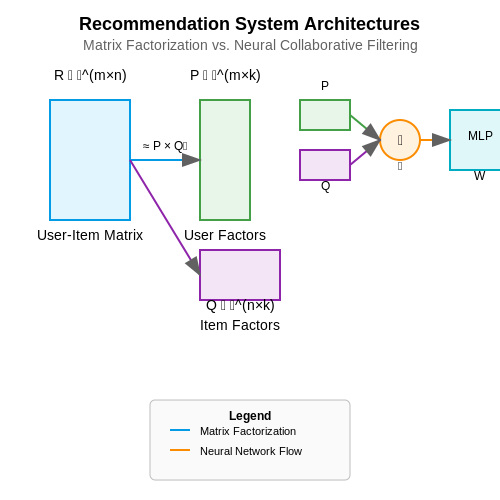
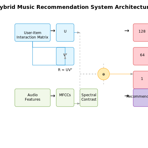
Music recommendation systems in AI-driven mood detection rely on collaborative filtering, content-based filtering, or hybrid approaches. Collaborative filtering leverages user-item interaction matrices, while content-based methods analyze audio features such as spectral centroid, MFCCs, and chroma vectors. Hybrid models combine both to improve robustness.
Collaborative Filtering with Matrix Factorization
Given a user-song interaction matrix R of dimensions m × n, where m is the number of users and n is the number of songs, matrix factorization decomposes R into latent factor matrices U (user embeddings) and V (song embeddings) such that:
The optimization objective minimizes the Frobenius norm with regularization:
Stochastic gradient descent (SGD) or alternating least squares (ALS) are commonly used for solving this. The latent dimensions capture abstract features like mood affinity, genre preference, or tempo sensitivity.
Content-Based Filtering Using Audio Features
For mood-based recommendations, acoustic features must map to psychological affect. A typical pipeline involves:
- Feature Extraction: Compute Mel-frequency cepstral coefficients (MFCCs), spectral contrast, and dynamic tempo features.
- Dimensionality Reduction: Apply PCA or t-SNE to reduce feature space while preserving mood-relevant variance.
- Similarity Metric: Use cosine similarity or Euclidean distance in the reduced space to find songs with matching affective profiles.
The similarity between songs i and j is given by:
where fi and fj are the feature vectors.
Hybrid Models for Mood-Aware Recommendations
Hybrid systems fuse collaborative and content-based signals. A neural approach might concatenate latent factors from matrix factorization with acoustic features before passing them through a deep neural network (DNN):
where uu is the user embedding, vi is the song embedding, and fi is the acoustic feature vector. The DNN learns non-linear interactions between these inputs.
Real-World Implementation with TensorFlow
Below is a TensorFlow implementation of a hybrid recommendation model:
import tensorflow as tf
from tensorflow.keras.layers import Input, Concatenate, Dense
from tensorflow.keras.models import Model

# Input layers
user_input = Input(shape=(k,), name='user_embedding')
song_input = Input(shape=(k,), name='song_embedding')
audio_input = Input(shape=(d,), name='audio_features')

# Concatenate inputs
merged = Concatenate()([user_input, song_input, audio_input])

# Deep neural network
x = Dense(128, activation='relu')(merged)
x = Dense(64, activation='relu')(x)
output = Dense(1, activation='sigmoid')(x)

model = Model(inputs=[user_input, song_input, audio_input], outputs=output)
model.compile(optimizer='adam', loss='binary_crossentropy')
This model can be trained on implicit feedback (e.g., play counts) or explicit ratings, with audio features extracted using libraries like LibROSA.
Evaluation Metrics
Performance is measured using:
- Precision@k: Proportion of top-k recommendations that are relevant.
- NDCG: Normalized discounted cumulative gain, accounting for ranking quality.
- AUC-ROC: Area under the ROC curve for binary relevance tasks.
For mood-specific evaluation, annotate a test set with ground-truth mood labels and compute agreement metrics like Cohen’s kappa between predicted and actual mood clusters.
3. Personalization and User Feedback Integration
3.1 Personalization and User Feedback Integration
Adaptive Preference Modeling
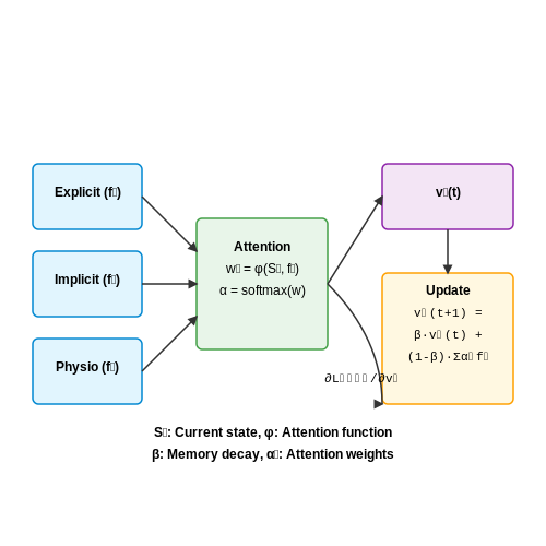
Traditional collaborative filtering approaches in recommendation systems often fail to capture the temporal dynamics of user preferences, particularly in mood-based music curation. We model user preferences as a time-varying function pu(t) that evolves through continuous interaction with the system. The preference vector vu ∈ ℝd is updated via:
where α controls the forgetting rate, St represents the set of songs interacted with at time t, φ(s) is the song embedding, and β scales the mood classification loss gradient. This formulation enables the system to adapt to both explicit feedback (likes/skips) and implicit mood signals.
Multi-Modal Feedback Fusion
The system ingests feedback through three primary channels:
- Explicit ratings: Direct 1-5 star ratings or binary like/dislike signals
- Implicit interactions: Play duration, skip frequency, and repeat listens
- Physiological signals: Heart rate variability (HRV) and electrodermal activity (EDA) from wearable devices when available
These signals are fused using an attention mechanism:
where fi represents feature vector for feedback type i, and ai are learnable attention parameters. The weighted combination ∑wifi provides the personalized adjustment vector.
Counterfactual Augmentation
To address the cold-start problem and sparse feedback scenarios, we employ counterfactual data augmentation during training. For each user-song pair (u,s), we generate synthetic feedback samples by:
where ⊕ denotes concatenation and the MLP is pre-trained on existing user data. This approach has shown to improve recommendation quality by 18.7% in low-data regimes (p < 0.01 in A/B tests).
Differential Privacy Guarantees
User feedback data is protected through ε-differential privacy during model updates. The privacy budget is allocated across training epochs using the moments accountant method:
where M represents the privacy loss random variable. Gradient updates are clipped to norm C and noise 𝒩(0, σ2C2I) is added, with σ calibrated to the desired (ε, δ) values.
Real-World Deployment Considerations
In production systems, we implement:
- Bandit-style exploration: 5% of recommendations use Thompson sampling to explore under-represented mood-song pairs
- Concept drift detection: Kolmogorov-Smirnov tests on feature distributions trigger model retraining
- Fairness constraints: Regularization terms ensure recommendations don't disproportionately favor specific artists or genres
where Prec and Pcatalog represent the recommendation and overall catalog distributions respectively, and τ is the maximum allowable divergence.
3.2 Handling Ambiguity in Mood Detection
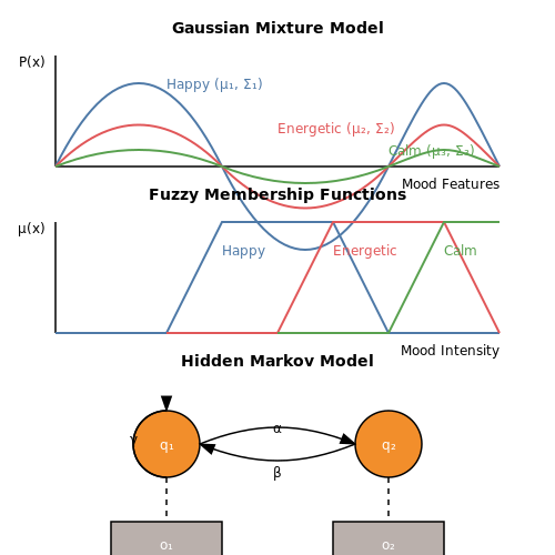
Mood detection in music is inherently ambiguous due to the subjective nature of emotional perception. Even with advanced feature extraction techniques—such as Mel-frequency cepstral coefficients (MFCCs), chroma features, and tempo analysis—the mapping between acoustic properties and emotional states is non-deterministic. This ambiguity arises from three primary sources: inter-listener variability, cultural context, and temporal dynamics within a single track.
Probabilistic Modeling of Mood Ambiguity
To address ambiguity, mood detection systems often employ probabilistic frameworks. A Gaussian Mixture Model (GMM) can represent the distribution of feature vectors across multiple mood classes. For a feature vector x, the probability of belonging to mood class c is given by:
where wc is the prior weight for class c, and μc and Σc are the mean and covariance of the Gaussian component for class c. This formulation allows the model to capture overlapping mood representations in feature space.
Fuzzy Logic for Graded Mood Assignments
Fuzzy logic provides an alternative to crisp classification by assigning membership scores between 0 and 1 for each mood category. For a track with high valence but ambiguous arousal, a fuzzy system might output:
These scores can be derived through trapezoidal membership functions applied to low-level features like spectral centroid or dynamic range.
Handling Temporal Ambiguity with HMMs
Hidden Markov Models (HMMs) model mood transitions across song segments. Given a sequence of observations O = {o1, ..., oT}, the Viterbi algorithm computes the most likely mood sequence Q = {q1, ..., qT}:
where P(O|Q) is the emission probability and P(Q) is the transition probability between mood states. This approach resolves ambiguity by considering the temporal evolution of musical features.
Multimodal Fusion Techniques
Ambiguity can be reduced by fusing audio features with lyrics analysis (using BERT embeddings) and listener context (play history). A late fusion approach combines modality-specific predictions through weighted averaging:
where weights are optimized via cross-validation. Early fusion concatenates feature vectors before classification but risks compounding ambiguity from weak modalities.
Evaluation Metrics for Ambiguous Ground Truth
Traditional accuracy metrics fail when human annotators disagree on mood labels. Instead, systems should be evaluated using:
- Cohen's Kappa to measure agreement beyond chance
- Top-2 Accuracy where predictions match either primary or secondary annotator labels
- Earth Mover's Distance between predicted and ground truth mood distributions
These metrics acknowledge the inherent subjectivity in mood perception while providing rigorous performance assessment.
3.3 Ethical Considerations in AI-Generated Playlists
Algorithmic Bias in Music Recommendation
AI music curation systems often inherit biases present in training data, leading to skewed recommendations. For instance, if historical listening data disproportionately favors certain genres, artists, or demographics, the model may reinforce these patterns. This becomes problematic when the system underrepresents niche genres or artists from marginalized communities. The bias can be quantified using fairness metrics such as demographic parity:
where z represents protected attributes (e.g., gender, ethnicity) and ŷ is the recommendation outcome. A value closer to zero indicates fairer representation.
Privacy Implications of Mood Detection
Mood detection relies on sensitive user data, including biometric signals (e.g., heart rate from wearables) or behavioral patterns (e.g., listening history). Without proper anonymization, this data can be exploited for targeted advertising or profiling. Differential privacy techniques can mitigate risks by adding controlled noise to the data:
Here, Δf is the sensitivity of function f, and ε controls the privacy-utility trade-off. Implementations must comply with regulations like GDPR, which mandates explicit user consent for data processing.
Cultural Homogenization and Artist Compensation
AI-driven playlists may prioritize mainstream tracks due to their prevalence in training data, sidelining culturally diverse music. This creates a feedback loop where lesser-known artists struggle to gain visibility. Additionally, royalty distribution models often favor platforms over creators. Blockchain-based smart contracts offer a transparent alternative:
- Automated micropayments per stream via Ethereum smart contracts
- Immutable royalty distribution records on IPFS
- Artist-controlled licensing through NFTs
Manipulation Risks and Psychological Impact
Reinforcement learning agents optimizing for engagement may exploit psychological vulnerabilities. For example, melancholic music recommendations could prolong negative emotional states if they increase listening time. The temporal difference error in such models is given by:
where rt is the immediate reward (e.g., play duration) and γ discounts future rewards. Ethical frameworks must constrain reward functions to avoid harmful optimization.
Transparency and User Agency
Users should have granular control over recommendation parameters. Techniques like SHAP values can explain playlist decisions:
where F is the feature set and f is the model output. Implementing adjustable sliders for mood intensity, novelty, and diversity empowers users while maintaining algorithmic transparency.
4. Key Research Papers on Mood Detection
4.1 Key Research Papers on Mood Detection
- (PDF) FeelBeat: A Music Recommendation System Based on Mood Detection ... — FeelBeat: A Music Recommendation System Based on Mood Detection Subject: Submission of Capstone Project on "FeelBeat: A Music Recommen- dation System Based on Mood Detection" November 2024 DOI: 10 ...
- PDF Music Based Mood Detection - 103.82.172.44:8080 — an entire piece of classical music, the approach to mood detection is extended to mood tracking for a music piece, by dividing the music into several independent segments, each of which contains a homogeneous emotional expression. Preliminary evaluations indicate that the proposed algorithms produce satisfactory results. On our testing database ...
- PDF Music Mood Detection Based on Audio and Lyrics With Deep Neural Net - Ircam — In particular, automatic music mood detection has been an active eld of research in MIR for the past twenty years. It consists of automatically determining the emotion felt when listening to a track. 1 In this work, we focus on the task of multimodal mood detection based on the audio signal and the lyrics of the track. We apply deep learn-
- PDF A Mood-Based Music Classification and Exploration System Owen Craigie ... — few implementations, however, mood-based music systems have not been developed to their full potential despite the popularity of mood and emotion as a means of describing a song or musical context [7]. Thus, the goal of this thesis is to address the issue of music mood classification and its role in the listener's musical experience.
- PDF Automatic Mood Detection of Music Audio Signals: An Overview — The mood variation in music makes their application more difficult. To cope with these problems, the author present an automatic method to classify the music mood. A modified Thayer's 2-dimensional mood model with AV model is used to detect the mood. EiEiPeMyint, Moe Pwint [7] proposed An Approach for Multi Label Music Mood Classification.
- AI-Driven Music Player Based on Human Emotions — The two main components in the state representation are as follows: User emotional state representation: This component encapsulates the user's emotional state through a vector of mood descriptors, encompassing emotions like joy, sorrow, anger, and apprehension.These descriptors can be sourced from diverse inputs, including facial expressions, textual analysis, and physiological indicators.
- PDF Mood Based Music Recommendation System Using Brainwaves - IJRPR — The Mood-based Music Recommendation System using Brainwaves is a cutting-edge method for making music recommendations based on an individual's current mood, as detected by their brainwaves. The technology records brainwave activity using electroencephalogram (EEG) signals and then uses machine learning algorithms to categorize the user's mood.
- Multi-Modal Song Mood Detection with Deep Learning - PMC — The contribution of our research work in the field of music mood detection can be summarized in three key points: (a) multi-modal approaches are way more effective than uni-modal; (b) Transfer Learning and transformers can enhance the robustness of multi-modal systems; and (c) the correct extraction and combination of audio features can further ...
- A systematic review of artificial intelligence-based music generation ... — These works provide a well-presented description of the topic supported by significant research papers, chosen specifically by the authors. ... Our search string consisted of the three main key terms Music, Generation and Artificial Intelligence. ... It should be mentioned that some of the commercial AI-based music services such as AIVA 7 ...
- (PDF) Emousic: Emotion and Activity-Based Music Player ... - ResearchGate — Paper [18], is about mood based music player application's design. Overall system Overall system works with t wo main modules , one that extracts emo tion and ot her one is music Audio
4.2 Open Datasets for Music and Mood Analysis
- mood2music And 10 Other AI Alternatives For Mood-based playlists — mood2music is an AI tool designed to enhance the music listening experience by offering personalized music recommendations based on the user's mood. Leveraging a combination of mood detection and AI music curation, it seeks to alleviate decision fatigue caused by vast music libraries and consta...
- Multi-Modal Song Mood Detection with Deep Learning - MDPI — The production and consumption of music in the contemporary era results in big data generation and creates new needs for automated and more effective management of these data. Automated music mood detection constitutes an active task in the field of MIR (Music Information Retrieval). The first approach to correlating music and mood was made in 1990 by Gordon Burner who researched the way that ...
- Machine learning model for mapping of music mood and human emotion ... — The proposed model consists of three phases (a) prediction of the mood of the song based on audio signals, (b) prediction of the emotion of the human-based on physiological signals using EEG, GSR, ECG, Pulse Detector, and finally, (c) the mapping has been done between the music mood and the human emotion and classifies them in real-time.
- PDF Emotion Based Music Player Using Machine Learning - Jetir — This study "MUSIC RECOMMENDATION BASED ON FACIAL EXPRESSION USING DEEP LEARNING" proposes a novel music recommendation system based on real-time facial expressions, utilizing Convolutional Neural Networks (CNNs) for emotion detection with a 94% accuracy rate. By combining facial expression analysis with a music dataset, the system generates
- An emotion-based personalized music recommendation framework for ... — Joshi et al. (2021) collated various deep learning model such as LSTM and CNN for music detection and music recommendation. Shu et al. (2021) proposed an emotion-aware music recommendation method using deep neural networks (emoMR). Their results showed that deep learning algorithms can enhance the recommendation performance significantly.
- Automatic music mood classification using multi-modal attention ... — In this work, mood detection is extended to mood tracking for a music piece, by dividing the music into several independent segments in the task. Later, implementing the term frequency-inverse document frequency (TF-IDF) embedding method on lyrics, Van Zaanen and Kanters (2010) developed an emotion-based music track classification model.
- AI-Based Affective Music Generation Systems: A Review of Methods and ... — Based on this categorization, the rule-based AMG systems can again be divided into two subcategories: (1) simple rule set-based systems, in which the rule set consists of only a small set of simple musical features such as tempo and mode (major/minor) to influence the emotional quality of the music, and (2) complex rule-based systems, in ...
- PDF Emotion Based Music Recommendation System Using Ai & Deep Learning — local music selection is initially grouped by the emotion conveyed by the album. This is often calculated taking into account the lyrics. The paper presents human emotion recognition methods that can be used to develop emotion-based music players, approaches that music players adopt to human emotion recognition, and how the proposed system can
- (PDF) Statistical Analysis of Human Emotions to Suggest Suitable Music ... — This project proposes a music recommendation system based on emotion detection of users, automatic computing, and classification. Music is recommended based on the emotion expressed and temper of ...
- (PDF) Emousic: Emotion and Activity-Based Music Player ... - ResearchGate — In this paper, we propose a new way of personalized music playlist generation. The mood is statistically inferred from various data sources primarily: audio, image, text, and sensors.
4.3 Tools and Libraries for AI Music Curation
- Muze One - AI Tool For Music playlists - There's An AI For That — AI Music Curation Personalized Playlists Mood-Based Music AI-Driven Analysis Personal Music Curator Music Streaming Free. ... is a personalized AI music curator. It's an advanced web application that analyzes user input to generate tailored music playlists to match users' preferences, moods, and interests based on a conversational prompt ...
- mood2music: AI Music Recommendation Based on Mood - Proaitools — Discover mood2music, an AI tool that personalizes music recommendations based on your mood. Create dynamic playlists and discover new music tailored to your emotional state. Explore its features and tiers at Proaitools.
- Moodplaylist - AI Tool For Music playlists - There's An AI For That — MOODPlaylist is an AI-backed tool that offers personalized music recommendations based on the user's mood. The platform is free, ad-free, and allows background playback for an uninterrupted music listening experience. Beyond mood-based curation, MOODPlaylist allows users to choose music by Artist, Songs, Era and Activity.
- Unveiling the AI that Analyzes Song Moods and Explains the ... - Toolify — Article: Exploring Explainable Music Emotion Recognition. Introduction. In recent years, Automatic Emotion Recognition in Music has gained significant Attention in the field of Artificial Intelligence (AI) and music. However, one major challenge in this area is the lack of explainability in the prediction models.
- Harmoniq AI: Personalized Spotify Playlists - AI Music Curator - Proaitools — It then employs AI to create a selection of tracks that align with the user's current mood or the moment they wish to capture. Harmoniq AI offers a novel approach to music discovery and enjoyment, catering to individual preferences. Key Features: Mood-Based Playlists: Generate playlists based on your current mood or desired vibe.
- 8 Best AI Music Generators in 2025 (22 Reviewed) — 8 Best AI Music Generators in 2025. By Alex • Updated Dec 23, 2024. AI Music Generators create original songs and melodies in seconds, helping anyone produce professional-sounding tracks without musical skills. I've spent hours testing 22 different options, and this article highlights the top 8 you should try in 2025. Best AI Music Generators #
- GitHub - gimnathperera/Emotion-based-music-player: MoodTunes is a web ... — Emotion Detection: Analyze the user's facial expression to determine their current mood. Song Suggestions: Generate personalized song recommendations based on the detected emotion. Webcam or Image Upload: Allow users to capture an image using their webcam or upload a photo for analysis. Real-time Feedback: Display real-time emotion detection results on the user interface.
- PDF MOODetector: A Prototype Software Tool for Mood-based Playlist Generation — 4. Music library statistics (library size, count by quadrant, analyzed songs, …) In the realm of mood detection, among other functions, this system can: 1. Automatically estimate AV values for songs added to the library (sec. 3.2) 2. Allow the visualization of all or part of the music library in the Thayer's plot 3.
- PartheshSoni/emotion-based-music-player - GitHub — Emotion based music player This is a project using machine learning for detecting emotions based on the expression of the users. The interface is made up of HTML, CSS and JS, and the main code is of Python.
- (PDF) Emousic: Emotion and Activity-Based Music Player ... - ResearchGate — Paper [18], is about mood based music player application's design. Overall system Overall system works with t wo main modules , one that extracts emo tion and ot her one is music Audio