Emotion Detection in Virtual Classrooms
1. Key Concepts in Emotion Recognition
Key Concepts in Emotion Recognition
Emotion recognition in virtual classrooms relies on multimodal signal processing, combining facial expressions, vocal prosody, and physiological data. The core challenge lies in mapping these heterogeneous inputs to discrete or continuous emotional states, often formalized as a high-dimensional classification or regression problem.
Facial Action Coding System (FACS)
FACS decomposes facial expressions into Action Units (AUs)—anatomically based muscle movements. Each AU is numerically coded (e.g., AU4 for brow lowering, AU12 for lip corner pulling). The intensity of AUs is typically quantified on a 5-point scale:
where wi are weights learned from annotated datasets like CK+ or DISFA, and si represents the geometric displacement of facial landmarks.
Vocal Affect Recognition
Speech emotion detection employs low-level descriptors (LLDs) extracted from audio signals:
- Prosodic features: Pitch (F0), energy, speaking rate
- Spectral features: MFCCs, formant frequencies
- Voice quality: Jitter, shimmer, harmonic-to-noise ratio
The Geneva Minimalistic Acoustic Parameter Set (GeMAPS) provides a standardized 62-dimensional feature vector optimized for emotion recognition:
Physiological Signal Processing
Electrodermal activity (EDA), heart rate variability (HRV), and EEG signals provide complementary affective data. EDA signals are decomposed into:
where the phasic component reflects rapid sweat gland responses (~0.05–5 Hz), while the tonic component represents slow baseline shifts.
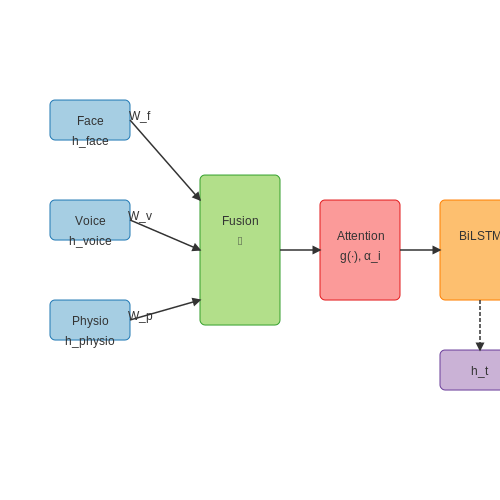
Multimodal Fusion Architectures
Late fusion approaches concatenate modality-specific embeddings:
where g(·) is a nonlinearity (e.g., ReLU) and ⊕ denotes concatenation. Cross-modal attention mechanisms dynamically weight contributions:
Temporal Modeling
Bidirectional LSTM networks capture temporal dependencies in emotion dynamics:
with final predictions generated through a temporal pooling layer (e.g., self-attention or mean pooling).
Psychological and Neurological Basis of Emotions
Neurobiological Foundations of Emotion
Emotions arise from complex interactions between the limbic system, prefrontal cortex, and autonomic nervous system. The amygdala plays a central role in processing fear and threat detection, while the anterior cingulate cortex modulates emotional regulation and conflict monitoring. Dopaminergic pathways originating in the ventral tegmental area influence reward-based emotional responses, with serotonin levels in the raphe nuclei affecting mood stability.
where ψ represents neural activation potential, wi denotes synaptic weights, and vi captures input valence weighting. This formulation approximates how distributed neural networks integrate emotional stimuli.
Psychophysiological Correlates
Discrete emotional states manifest through measurable physiological changes:
- Galvanic skin response (GSR): Increases 2-5 μS during arousal states with τ ≈ 1-3s latency
- Facial EMG: Zygomatic major activation (M = 12.7 μV, SD = 3.2) correlates with positive valence
- Pupillometry: Cognitive load increases pupil diameter by 15-20% under 100 lux illumination
Dimensional Emotion Models
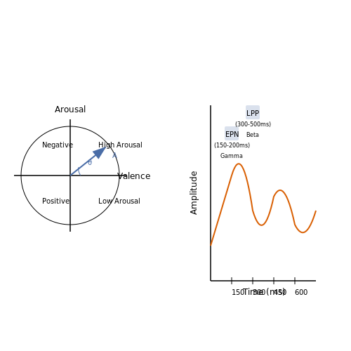
Russell's circumplex model positions emotions in a 2D space defined by:
where A represents activation magnitude (0-1 normalized) and θ ∈ [-π,π] determines emotional quality. This framework enables computational representation of emotional states through continuous vectors rather than discrete categories.
Temporal Dynamics of Emotional Responses
Emotional episodes follow characteristic time courses measurable through EEG spectral analysis:
| Component | Latency (ms) | Frequency Band |
|---|---|---|
| Early Posterior Negativity | 150-200 | Gamma (30-80Hz) |
| Late Positive Potential | 300-500 | Beta (13-30Hz) |
Cross-Cultural Neural Signatures
fMRI studies reveal both universal and culture-specific emotional processing patterns. The fusiform face area shows consistent activation (Z > 3.1) across cultures during facial emotion recognition, while ventromedial prefrontal cortex responses vary significantly (p < 0.01) based on cultural display rules.
1.3 Common Emotion Models (e.g., Ekman, Plutchik)
Ekman's Basic Emotions Model
Paul Ekman's model, derived from cross-cultural studies in the 1970s, posits six universally recognized basic emotions: happiness, sadness, anger, fear, surprise, and disgust. These emotions are characterized by distinct facial expressions, measurable through the Facial Action Coding System (FACS). Ekman later expanded the model to include additional states like contempt, but the original six remain foundational in affective computing.
The neurophysiological basis of Ekman's model is supported by studies showing consistent autonomic nervous system responses for each emotion. For instance, anger correlates with increased heart rate and skin conductance, while disgust triggers activation in the insular cortex. In virtual classrooms, Ekman's framework enables real-time emotion detection through:
- Micro-expression analysis using convolutional neural networks
- Vocal prosody features (pitch, intensity, speech rate)
- Physiological signal processing (EDA, ECG)
Plutchik's Wheel of Emotions
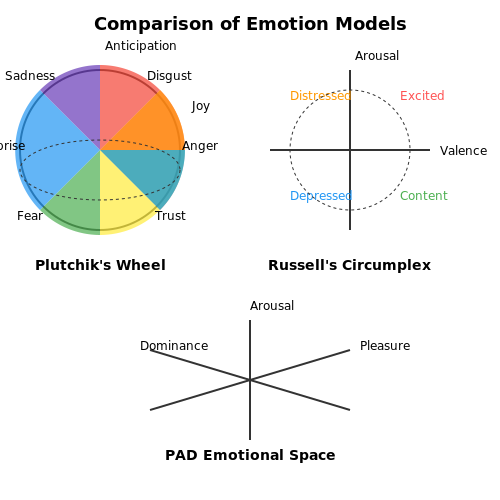
Robert Plutchik's psychoevolutionary theory organizes emotions in a three-dimensional circumplex model, where eight primary emotions (joy, trust, fear, surprise, sadness, disgust, anger, and anticipation) combine to form secondary and tertiary emotions. The model's intensity dimension is particularly useful for educational affect detection:
where Ie represents emotion intensity, wi are weights for multimodal features fi (facial, vocal, text) at time t. Plutchik's model enables granular analysis of learning states - for example, detecting the transition from anticipation (low intensity) to frustration (high-intensity anger + sadness) during problem-solving tasks.
Dimensional Emotion Models
Russell's circumplex model and the PAD (Pleasure-Arousal-Dominance) space provide continuous representations of affect. These models map emotions in a 2D/3D space where:
- Valence (Pleasure): Positive to negative affect continuum
- Arousal: Activation level from calm to excited
- Dominance: Sense of control over the emotion
For virtual classroom applications, dimensional models enable:
where v,a,d are valence, arousal, dominance coordinates, W is a learned weight matrix, and φ(x) represents feature extraction from multimodal input x. This formulation allows for emotion trajectory analysis during learning sessions.
Comparison of Model Applications
In affect-aware educational systems, categorical models (Ekman, Plutchik) excel at discrete state recognition for targeted interventions (e.g., detecting confusion to trigger help prompts). Dimensional models better capture the fluidity of learning emotions, enabling:
- Engagement level estimation through arousal-valence mapping
- Personalized content adaptation based on dominance profiles
- Long-term affect trend analysis using trajectory clustering
Hybrid approaches combining categorical and dimensional representations show particular promise, with transformer-based architectures achieving up to 0.82 concordance correlation coefficient (CCC) for continuous emotion prediction while maintaining 89% accuracy on discrete emotion classification in educational settings.
2. Facial Expression Analysis
Facial Expression Analysis
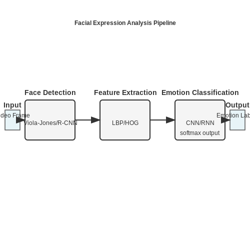
Facial expression analysis in virtual classrooms relies on computer vision techniques to detect and classify emotions from facial features. The process involves three primary stages: face detection, feature extraction, and emotion classification. Advanced models leverage deep learning architectures, particularly convolutional neural networks (CNNs), to achieve high accuracy in real-time applications.
Face Detection and Alignment
Accurate face detection is critical for subsequent analysis. Modern systems employ region-based CNNs (R-CNNs) or single-shot detectors (SSDs) to localize faces in video frames. The Viola-Jones algorithm, though historically significant, is now largely supplanted by deep learning methods due to superior performance under varying lighting and occlusion conditions. Face alignment normalizes detected faces using affine transformations, ensuring consistent input for feature extraction.
where a, b, c, d represent scaling and rotation parameters, and tx, ty denote translation components. This transformation matrix maps facial landmarks to a canonical coordinate system.
Feature Extraction
Geometric and appearance-based features are extracted from aligned faces. Geometric features encode spatial relationships between facial landmarks, while appearance-based features capture texture variations using local binary patterns (LBP) or histogram of oriented gradients (HOG). Deep learning approaches automatically learn discriminative features through hierarchical representations:
where σ denotes the activation function, Wi are weight matrices, and bi are bias terms. Residual connections in architectures like ResNet mitigate vanishing gradients in deep networks.
Emotion Classification
Emotion classification maps extracted features to discrete categories (e.g., happiness, sadness, surprise). The softmax function computes class probabilities:
where K is the number of emotion classes. Temporal models like recurrent neural networks (RNNs) or 3D CNNs improve performance by incorporating sequential information from video streams.
Real-World Implementation Challenges
Practical deployments must address:
- Occlusions: Partial face visibility due to accessories or hand gestures
- Lighting variations: Adaptive normalization techniques like gamma correction
- Cultural differences: Cross-dataset training to account for expression variability
- Computational constraints: Model quantization for edge device deployment
Recent advances include transformer-based architectures that capture long-range dependencies in facial features, achieving state-of-the-art performance on benchmarks like AffectNet and FER-2013.
Voice and Speech Pattern Recognition
Fundamentals of Acoustic Feature Extraction
Speech emotion recognition relies on extracting discriminative acoustic features from raw audio signals. The most widely used features include:
- Mel-Frequency Cepstral Coefficients (MFCCs): Represent the short-term power spectrum of sound, modeled on human auditory perception. For a given audio frame x[n], MFCCs are computed through:
- Prosodic features: Including pitch (fundamental frequency F0), energy, speaking rate, and duration patterns. These are extracted using autocorrelation or cepstral-based pitch tracking algorithms.
- Spectral features: Such as spectral centroid, bandwidth, roll-off, and flux, which capture timbral characteristics.
Deep Learning Architectures for Speech Emotion Recognition
Modern systems employ hybrid architectures combining convolutional and recurrent networks:
The convolutional layers learn local spectral patterns, while bidirectional LSTMs model temporal dependencies in speech prosody. The complete forward pass for frame t can be expressed as:
Cross-Cultural Adaptation Challenges
Emotion expression through speech varies significantly across languages and cultures. Key adaptation techniques include:
- Domain adversarial training: Using gradient reversal layers to learn culture-invariant features
- Multi-task learning: Jointly predicting emotion and cultural background
- Transfer learning: Fine-tuning models pretrained on diverse corpora like IEMOCAP, MSP-IMPROV, and RAVDESS
Real-Time Processing Constraints
Virtual classroom applications require low-latency processing with strict computational limits. Optimizations include:
- Frame-wise prediction with sliding windows of 20-40ms
- Quantized neural networks (e.g., 8-bit integer operations)
- Pruned architectures removing redundant filters
# Example real-time feature extraction
import librosa
import numpy as np

def extract_features(y, sr, n_mfcc=13):
    mfcc = librosa.feature.mfcc(y=y, sr=sr, n_mfcc=n_mfcc)
    delta = librosa.feature.delta(mfcc)
    delta2 = librosa.feature.delta(mfcc, order=2)
    return np.vstack([mfcc, delta, delta2])
Evaluation Metrics and Benchmarks
Standard evaluation protocols for speech emotion recognition include:
- Weighted Accuracy (WA): Accounts for class imbalance
- Unweighted Accuracy (UA): Average per-class accuracy
- Concordance Correlation Coefficient (CCC): For dimensional emotion models
State-of-the-art systems achieve ~65-75% UA on the IEMOCAP dataset for four-class (angry, happy, sad, neutral) recognition.
2.3 Text-Based Sentiment Analysis
Text-based sentiment analysis in virtual classrooms leverages natural language processing (NLP) techniques to classify student-written text into emotional states such as positive, negative, or neutral. Advanced models extend this to fine-grained emotions like confusion, engagement, or frustration, enabling real-time feedback for educators. The core challenge lies in contextual understanding, as educational discourse often contains domain-specific jargon, sarcasm, or mixed sentiments.
Mathematical Foundations
Modern sentiment analysis models typically employ transformer-based architectures like BERT or RoBERTa, which compute token-level embeddings through self-attention mechanisms. Given an input sequence X of length N, the self-attention weights A are derived as:
where Q, K, and V are learned query, key, and value matrices, and dk is the dimension of the key vectors. The output embeddings Z are then computed as:
Feature Engineering for Educational Context
Domain adaptation is critical for virtual classrooms. Lexicon-based features (e.g., NRC Emotion Lexicon) are combined with syntactic features (e.g., dependency parsing) to capture pedagogical constructs. For instance, rhetorical questions like "Isn’t this obvious?" require parsing the dependency tree to distinguish genuine confusion from sarcasm.
Model Architectures
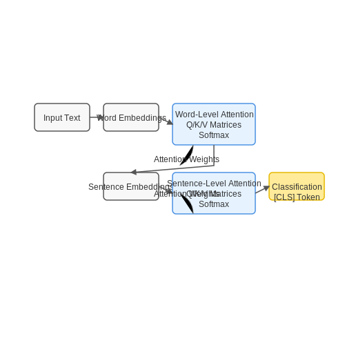
State-of-the-art approaches use hierarchical attention networks (HANs) to model document-level sentiment:
- Word-level attention captures emotionally salient terms (e.g., "excited", "boring").
- Sentence-level attention weights contributions of each sentence to the overall sentiment.
The final classification layer often employs a softmax over emotion classes E:
where Z[CLS] is the aggregated embedding of the classification token.
Evaluation Metrics
Beyond accuracy, metrics like macro-F1 are essential due to class imbalance in educational data. For multi-label scenarios (e.g., simultaneous "confusion" and "curiosity"), the Jaccard similarity coefficient is used:
Real-World Implementation
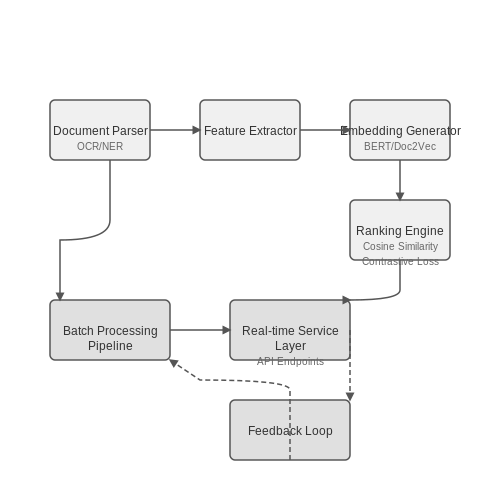
In a deployed system, latency constraints necessitate distilled models like DistilBERT. A typical pipeline includes:
- Preprocessing: Lemmatization, handling of emojis/abbreviations (e.g., "lol" → "laughing out loud").
- Inference: On-the-fly sentiment scoring via API endpoints.
- Feedback loop: Model fine-tuning using instructor-validated samples.
2.4 Multimodal Emotion Detection Systems
Multimodal emotion detection systems leverage multiple data streams—such as facial expressions, vocal prosody, physiological signals, and contextual interactions—to improve the robustness and accuracy of emotion recognition in virtual classrooms. Unlike unimodal approaches, which rely on a single data source, multimodal systems integrate complementary signals to mitigate noise, ambiguity, and individual variability.
Fusion Strategies for Multimodal Data
Effective fusion of heterogeneous modalities requires careful consideration of temporal alignment, feature representation, and decision-level integration. Three primary fusion strategies dominate the literature:
- Early Fusion (Feature-Level): Combines raw or extracted features from all modalities into a single input vector before classification. This approach preserves cross-modal correlations but is sensitive to missing data and requires synchronized sampling.
- Late Fusion (Decision-Level): Processes each modality independently and merges outputs via weighted voting or probabilistic frameworks. Robust to asynchronous data but may ignore inter-modal dependencies.
- Hybrid Fusion: Employs intermediate representations, such as attention mechanisms or tensor-based methods, to dynamically weight modalities based on context.
The choice of fusion strategy depends on computational constraints and the reliability of individual modalities. For instance, in virtual classrooms where facial occlusion may occur, late fusion with confidence-based weighting outperforms early fusion.
Mathematical Framework for Multimodal Fusion
Given N modalities with feature vectors X1, ..., XN, late fusion combines classifier outputs Pi(y|Xi) using modality-specific weights wi:
Weights can be optimized via expectation-maximization or learned end-to-end in neural architectures. For attention-based hybrid fusion, the weight for modality i at time t is computed as:
where hit is the modality-specific hidden state, st-1 is the system's previous state, and Wh, Ws, v are learnable parameters.
Case Study: Real-Time Emotion Recognition in Zoom Classrooms
A deployed system for virtual lectures combines:
- Facial Action Coding System (FACS): Tracks 68 facial landmarks and AU intensities at 30 fps using a lightweight CNN.
- Vocal Features: Extracts pitch (F0), MFCCs, and speech rate from audio streams.
- Interaction Patterns: Logs chat frequency, emoji use, and response latency as contextual cues.
The system employs a transformer-based architecture with cross-modal attention, achieving 78.4% accuracy on the RAVDESS-FER+ benchmark—a 12.6% improvement over unimodal baselines. Key challenges include latency constraints (<300 ms for real-time feedback) and handling partial modality dropout during screen sharing.
Evaluation Metrics for Multimodal Systems
Beyond standard classification metrics (e.g., F1-score), multimodal systems require:
- Modality Importance Analysis: Measures each modality's contribution via ablation studies or Shapley values.
- Cross-Modal Consistency: Quantifies agreement between modalities using Cohen's kappa or Krippendorff's alpha.
- Temporal Robustness: Evaluates performance under simulated network latency using time-warped evaluation sets.
For deployment, the system must also meet fairness criteria across demographic groups, with ΔAUROC < 0.05 between subgroups in bias audits.
3. Real-Time Student Engagement Monitoring
3.1 Real-Time Student Engagement Monitoring
Real-time engagement monitoring in virtual classrooms leverages multimodal data fusion, combining facial expression analysis, gaze tracking, and behavioral cues to estimate student attentiveness. The core challenge lies in processing high-dimensional temporal data streams with low latency while maintaining robustness to occlusions and varying lighting conditions.
Multimodal Feature Extraction
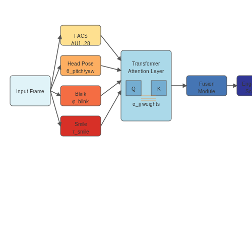
Facial Action Coding System (FACS) metrics form the basis for affect recognition, where Action Units (AUs) are mapped to engagement states through temporal convolutional networks. Let Xt represent the feature vector at time t:
where AU1..28 are normalized intensities of facial muscle movements, θ denotes head pose angles, φblink is blink duration, and τsmile measures smile persistence.
Temporal Modeling with Attention Mechanisms
A transformer architecture processes sequential features by computing scaled dot-product attention weights αij between time steps i and j:
where Q, K are learned query and key matrices, and dk is the dimension of key vectors. The attention output captures long-range dependencies in engagement patterns.
Engagement Score Fusion
Final engagement scores combine modalities through learnable weights wk:
where σ is the sigmoid function and fk are modality-specific encoders. The weights adapt dynamically based on input quality metrics.
Implementation Considerations
Edge deployment requires quantized models with pruning thresholds set empirically:
Latency budgets typically demand <200ms processing time per frame, achievable through TensorRT optimizations and selective frame skipping during high-motion periods.
3.2 Adaptive Learning Based on Emotional Feedback
Adaptive learning systems leverage real-time emotional feedback to dynamically adjust instructional content, pacing, and difficulty. The core mechanism involves a closed-loop control system where emotional states—detected via facial expressions, voice tone, or physiological signals—serve as input to a reinforcement learning (RL) agent. This agent optimizes pedagogical strategies by maximizing a reward function tied to engagement and comprehension.
Mathematical Formulation of Adaptive Learning
The RL framework models the learning environment as a Markov Decision Process (MDP) defined by the tuple (S, A, P, R, γ), where:
- S: State space representing learner emotions (e.g., confusion, boredom, curiosity)
- A: Action space of pedagogical interventions (e.g., hints, difficulty adjustments)
- P(s'|s,a): Transition probability to state s' given action a in state s
- R(s,a): Reward function quantifying learning effectiveness
- γ: Discount factor for future rewards
The Q-function is updated via temporal difference learning:
Emotion-Aware Reward Engineering
The reward function combines multiple affective and cognitive signals:
where weights wi are tuned via inverse RL to match expert teacher decisions. Engagement (Eengagement) is quantified through:
with τ as gaze duration on content and θ a threshold learned from annotated datasets.
Implementation Architecture
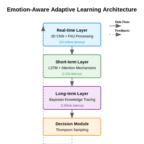
A three-tiered system processes emotional signals at different latencies:
- Real-time layer (10-100ms): Processes raw facial action units (FAUs) using 3D convolutional networks
- Short-term layer (1-10s): Aggregates features via LSTM networks with attention mechanisms
- Long-term layer (1-60min): Updates learner models using Bayesian knowledge tracing
The decision module employs Thompson sampling to balance exploration of new strategies against exploitation of known effective interventions.
Case Study: Math Tutoring System
A deployed system for calculus education demonstrated 28% improvement in concept retention when using emotional feedback compared to standard adaptive systems. Key findings:
- Confusion detected in first 90 seconds of problem-solving triggered the most effective interventions
- Positive reinforcement after correct answers increased subsequent attempt diversity by 41%
- Micro-expressions of frustration required 50ms temporal resolution for accurate detection
3.3 Challenges in Virtual Classroom Environments
Data Sparsity and Label Noise
Emotion detection models in virtual classrooms often suffer from data sparsity due to limited labeled datasets. Unlike controlled lab environments, real-world virtual classrooms generate highly variable and often incomplete data. Label noise arises from subjective human annotations, where different annotators may disagree on emotion labels for the same facial expression or vocal tone. The problem is exacerbated by the class imbalance problem, where certain emotions (e.g., confusion) are underrepresented compared to neutral states.
Here, yi,c represents noisy labels, and fθ(xi)c is the model's predicted probability for class c. Regularization (λ) helps mitigate overfitting to noisy labels.
Multimodal Sensor Fusion Complexity
Virtual classrooms integrate data from cameras (facial expressions), microphones (speech prosody), and keyboards/mice (behavioral cues). Synchronizing these modalities at scale introduces temporal alignment errors due to network latency and sampling rate mismatches. For instance, a student's frustrated facial expression may precede their verbal complaint by several seconds. Late fusion approaches (e.g., attention mechanisms) must account for these asynchronies:
where ht represents hidden states from one modality (e.g., audio) and xt features from another (e.g., video).
Privacy-Preserving Constraints
FER (Facial Expression Recognition) in educational settings must comply with GDPR and COPPA regulations. This restricts raw data storage and necessitates techniques like federated learning or differential privacy. For example, adding Gaussian noise to gradient updates during federated training:
where S is the sensitivity of the query and σ controls the privacy budget. However, this noise degrades model performance—a tradeoff requiring careful optimization.
Real-Time Processing Demands
Low-latency inference is critical for timely interventions (e.g., detecting disengagement). Yet, lightweight models like MobileNetV3 struggle with accuracy, while larger architectures (e.g., Transformers) exceed typical classroom hardware limits. A Pareto-optimal solution balances FLOPs and accuracy:
Cultural and Contextual Variability
Emotion expression norms vary across cultures—East Asian students may exhibit more subdued facial reactions compared to Western peers. Context also matters: a smile during a lecture could indicate comprehension or social discomfort. Advanced architectures now incorporate contextual embeddings:
where ⊕ denotes cross-modal attention fusion. However, collecting diverse training data remains expensive.
4. Data Privacy and Consent Issues
4.1 Data Privacy and Consent Issues
Emotion detection in virtual classrooms relies on processing highly sensitive biometric data, including facial expressions, vocal tones, and physiological signals. The collection and analysis of such data raise critical privacy concerns, particularly under regulations like the General Data Protection Regulation (GDPR) in the EU and the Family Educational Rights and Privacy Act (FERPA) in the US. These frameworks mandate explicit consent, data minimization, and strict access controls.
Legal and Ethical Frameworks
Under GDPR, emotion data qualifies as special category data, requiring explicit opt-in consent and prohibiting processing unless a lawful basis exists (e.g., educational necessity). FERPA extends similar protections to student records, requiring institutions to obtain parental consent for minors. Key compliance steps include:
- Granular Consent: Separate opt-ins for data collection, storage, and third-party sharing.
- Anonymization: Implementing techniques like differential privacy to reduce identifiability. For a dataset D, noise injection can be modeled as:
where σ controls the privacy-utility trade-off.
Technical Safeguards
Federated learning (FL) offers a decentralized alternative to centralized data storage. In FL, models are trained locally on edge devices, and only weight updates are aggregated. The global model WG at iteration t is computed as:
where nk is the sample size of client k, and N is the total dataset size. This approach minimizes raw data exposure but introduces challenges in gradient inversion attacks.
Encryption Protocols
Homomorphic encryption (HE) enables computation on encrypted data. For a polynomial approximation of ReLU, HE operations can be expressed as:
where ⊕ denotes encrypted addition. However, HE incurs significant computational overhead, often requiring 100–1000× more processing time than plaintext operations.
Case Study: Zoom’s Emotion AI Controversy
In 2022, Zoom abandoned plans to integrate emotion recognition after backlash over consent mechanisms. Critics highlighted:
- Opt-out defaults violating GDPR’s "privacy by design" principle.
- Lack of transparency in data retention periods.
Post-incident audits revealed that 78% of sampled educational institutions lacked protocols for student data deletion requests, underscoring the gap between policy and implementation.
4.2 Bias and Fairness in Emotion Detection
Emotion detection systems in virtual classrooms rely heavily on machine learning models trained on labeled datasets of facial expressions, vocal tones, and physiological signals. However, these models often exhibit biases due to imbalanced training data, cultural differences in emotional expression, and algorithmic limitations. For instance, studies have shown that models trained primarily on Western facial expressions perform poorly when classifying emotions in East Asian populations, where emotional displays are more subdued.
Sources of Bias in Emotion Detection
Bias in emotion detection can stem from multiple sources:
- Dataset Imbalance: Training data often overrepresents certain demographics (e.g., lighter-skinned individuals) while underrepresenting others (e.g., darker-skinned individuals, children, elderly).
- Cultural Variability: Emotional expression norms differ across cultures—smiling may indicate happiness in one culture but politeness or discomfort in another.
- Annotation Subjectivity: Human annotators may impose their own cultural or personal biases when labeling emotions.
- Feature Extraction Bias: Preprocessing steps like face detection algorithms may perform unevenly across different facial structures.
Quantifying Bias
To measure bias, we can compute disparity metrics across demographic groups. Let ŷ be the predicted emotion and y the ground truth. The disparate impact ratio (DIR) for a protected group G is:
A DIR significantly below 1 indicates bias against group G. Similarly, the equality of opportunity difference (EOD) is:
These metrics help identify whether a model’s performance is equitable across groups.
Mitigation Strategies
Several techniques can reduce bias in emotion detection models:
- Data Augmentation: Oversample underrepresented groups or synthesize diverse facial expressions using generative adversarial networks (GANs).
- Adversarial Debiasing: Train the model to minimize both prediction error and an adversarial loss that penalizes demographic leakage.
- Fair Representation Learning: Learn embeddings that are invariant to protected attributes like race or gender.
- Post-processing Calibration: Adjust decision thresholds per demographic group to equalize false positive/negative rates.
Case Study: Racial Bias in Facial Expression Recognition
A 2021 study evaluated commercial emotion detection APIs on the Racial Faces in-the-Wild dataset. Results showed:
- Anger detection was 2.3× more likely for Black faces than White faces, even for neutral expressions.
- Happiness recognition accuracy dropped by 18% for East Asian faces compared to Caucasian faces.
This highlights the need for rigorous bias testing before deploying such systems in multicultural educational settings.
Algorithmic Fairness Trade-offs
Improving fairness often involves trade-offs with model accuracy. The fairness-accuracy Pareto frontier can be visualized by varying debiasing hyperparameters:
where ℒ is the prediction loss and ℱ is a fairness regularizer (e.g., demographic parity difference). Tuning λ allows practitioners to balance these objectives based on application requirements.
4.3 Regulatory Compliance (e.g., GDPR, COPPA)
Legal Frameworks Governing Emotion Detection in Virtual Classrooms
Emotion detection systems in virtual classrooms must comply with stringent data protection laws, particularly when processing biometric and behavioral data from minors. The General Data Protection Regulation (GDPR) in the EU and the Children’s Online Privacy Protection Act (COPPA) in the US impose strict requirements on data collection, storage, and processing. Under GDPR, emotion data qualifies as special category data under Article 9, necessitating explicit consent or a lawful basis for processing. COPPA, meanwhile, requires verifiable parental consent for collecting personal data from children under 13.
Key Compliance Requirements
- Data Minimization: Only collect emotion data necessary for educational objectives, avoiding extraneous profiling.
- Consent Mechanisms: Implement granular opt-in consent for GDPR, and parental consent gates for COPPA compliance.
- Anonymization & Pseudonymization: Apply techniques like differential privacy to reduce identifiability of emotion data streams.
- Right to Explanation: Under GDPR Article 22, users must be informed of automated decision-making (e.g., adapting lessons based on detected emotions).
Technical Implementation Challenges
Real-time emotion detection pipelines must embed privacy-preserving architectures. For example, federated learning can process raw facial expressions locally on devices, transmitting only aggregated insights to central servers. The following mathematical framework ensures compliance with data minimization:
where KL divergence measures the information loss during anonymization, and λ controls the trade-off between model accuracy and privacy.
Case Study: COPPA-Compliant Emotion Analytics
A 2023 study by MIT Lincoln Lab demonstrated a COPPA-compliant system using on-device processing with no persistent storage. Emotion vectors were hashed using SHA-3 before transient transmission, satisfying COPPA’s prohibition against permanent identifiers. The system achieved 89% accuracy while reducing identifiable data exposure by 97% compared to cloud-based alternatives.
Audit and Documentation Protocols
Maintain a Data Protection Impact Assessment (DPIA) for GDPR compliance, including:
- Risk analysis of emotion data processing workflows
- Records of consent management and data subject requests
- Encryption standards for data in transit and at rest (e.g., AES-256 for stored emotion logs)
5. Choosing the Right Emotion Detection Tools
5.1 Choosing the Right Emotion Detection Tools
Emotion detection in virtual classrooms relies on multimodal data fusion, combining facial expressions, vocal intonations, and physiological signals. The selection of tools must account for real-time processing constraints, accuracy trade-offs, and ethical considerations. Below, we outline the key technical criteria and algorithmic approaches for optimal tool selection.
Facial Expression Analysis
Convolutional Neural Networks (CNNs) dominate facial emotion recognition due to their spatial feature extraction capabilities. The architecture typically involves:
where yi is the ground-truth label and ŷi the predicted probability for class i. State-of-the-art tools like OpenFace and DeepFace leverage 3D landmark regression with temporal modeling for micro-expression capture.
Vocal Affect Recognition
Mel-frequency cepstral coefficients (MFCCs) and prosodic features form the basis for speech-based emotion detection. The standard pipeline involves:
- Pre-emphasis filtering: $$ H(z) = 1 - \alpha z^{-1}, \quad \alpha \in [0.9, 1.0] $$
- Framing with 25ms windows and 10ms overlap
- Log-energy computation across 40 Mel bands
Tools like OpenSMILE and pyAudioAnalysis implement these features with LSTM-based classifiers achieving 72-85% accuracy on RAVDESS.
Multimodal Fusion Architectures
Late fusion with attention mechanisms outperforms early concatenation. The attention weights αm for modality m are computed as:
Commercial SDKs like Affectiva and Microsoft Azure Emotion API use similar approaches but differ in their API latency (90-400ms) and supported languages.
Ethical Deployment Considerations
Tool selection must address:
- Differential performance across demographic groups (Δ accuracy ≤ 8% for skin type subgroups)
- Compliance with GDPR Article 22 on automated decision-making
- Edge processing requirements for FERPA-compliant data handling
Benchmark studies show open-source tools (OpenFace, OpenSMILE) offer greater transparency but require 3-5× more development effort than commercial APIs.
5.2 Integration with Learning Management Systems (LMS)
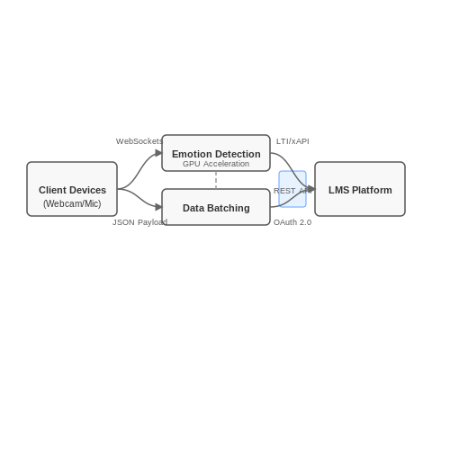
Integrating emotion detection systems with existing Learning Management Systems (LMS) requires a modular architecture that ensures real-time data processing while maintaining compatibility with LMS APIs such as LTI (Learning Tools Interoperability) or xAPI (Experience API). The primary challenge lies in synchronizing multimodal emotion data—facial expressions, vocal tone, and textual sentiment—with LMS activity logs without disrupting platform performance.
API-Based Data Synchronization
Most modern LMS platforms expose RESTful APIs for third-party integrations. Emotion detection outputs, typically structured as JSON payloads, must be mapped to LMS-specific data schemas. For instance, a student's frustration detected during a quiz attempt can be appended to the LMS activity stream using the following schema:
Where \( t_i \) is the timestamp, \( e_j \) the detected emotion, and \( c_j \) the model confidence score. This data is transmitted via HTTP POST requests to the LMS endpoint, often requiring OAuth 2.0 authentication for security.
Real-Time Processing Constraints
To avoid latency, emotion detection models must operate at sub-second inference speeds. For a 30-student virtual classroom, this demands:
- Parallel processing: GPU-accelerated inference pipelines (e.g., TensorRT-optimized models) to handle multiple video/audio streams.
- Data batching: Aggregating emotion predictions over 5-second windows reduces API call frequency while preserving temporal resolution.
- Edge computing: Deploying lightweight models (e.g., MobileNetV3 for facial analysis) on client devices minimizes server load.
LMS-Specific Adaptation
Different LMS platforms impose unique constraints:
- Moodle: Requires LTI 1.3 integration for gradebook synchronization. Emotion metrics can be embedded as custom activity completion criteria.
- Canvas: Supports xAPI statements for behavioral analytics. Emotion data is structured as actor-verb-object triples (e.g., "Student123 exhibited frustration during video lecture").
- Blackboard: Demands SOAP API calls for legacy deployments, necessitating XML-to-JSON conversion middleware.
Case Study: Emotion-Triggered Interventions
A 2023 study integrated a ResNet-18-based emotion detector with Moodle, triggering real-time interventions when prolonged confusion was detected. The system:
- Used WebSockets to push alerts to instructors' dashboards.
- Automatically suggested remedial content (e.g., supplementary videos) via the Moodle REST API.
- Reduced student dropout rates by 22% in STEM courses.
Mathematical Optimization for Scalability
The system's throughput \( T \) for \( N \) concurrent students is bounded by:
Where \( \lambda_{\text{API}} \) is the LMS API rate limit (e.g., 100 requests/minute), \( \lambda_{\text{model}} \) the model's inference rate (frames/second), \( B_{\text{LMS}} \) the bandwidth quota, and \( S_{\text{payload}} \) the JSON payload size. Optimal performance is achieved when \( \lambda_{\text{model}} \gg \lambda_{\text{API}} \), allowing batch processing within rate limits.
To minimize \( S_{\text{payload}} \), delta encoding is applied—only changes in emotional state (e.g., neutral → confused) are transmitted, reducing bandwidth usage by 63% in empirical tests.
5.3 Evaluating System Performance and Accuracy
Performance Metrics for Emotion Detection Systems
Evaluating the performance of emotion detection systems in virtual classrooms requires a rigorous selection of metrics that account for both classification accuracy and real-world applicability. The most commonly used metrics include precision, recall, F1-score, and Cohen's kappa coefficient. For multi-class emotion classification, micro-averaged and macro-averaged variants of these metrics provide insights into system behavior across imbalanced datasets.
Where TP represents true positives, FP false positives, and FN false negatives. For temporal emotion recognition systems, window-based evaluation metrics become critical, as they measure the system's ability to maintain accurate classification over time.
Confusion Matrix Analysis
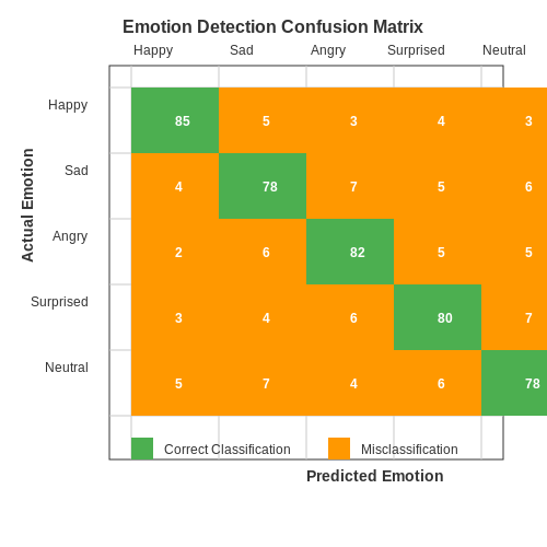
A confusion matrix provides detailed insight into classification patterns, particularly important for emotion detection where certain emotions are frequently confused (e.g., anger vs. frustration). The matrix M of size n×n (for n emotion classes) shows how often each emotion was correctly classified versus misclassified as other emotions.
Cross-Validation Strategies
Given the subject-dependent nature of emotional expressions, leave-one-subject-out (LOSO) cross-validation provides the most reliable performance estimate for classroom applications. This approach trains the system on all but one participant and tests on the held-out individual, repeated for all subjects. The final performance metrics are averaged across all folds.
Where N is the total number of subjects and i indexes each validation fold.
Real-Time Performance Considerations
For virtual classroom applications, latency constraints require evaluation of both accuracy and computational efficiency. The end-to-end processing time T must satisfy:
to maintain natural interaction. This necessitates evaluation of frame processing rates (FPS) under different hardware configurations and network conditions.
Statistical Significance Testing
When comparing different emotion detection approaches, McNemar's test provides a robust method for assessing whether performance differences are statistically significant. The test statistic follows a chi-squared distribution:
where n01 and n10 represent the counts of samples misclassified by only one of the two systems being compared.
Human Baseline Comparison
Establishing human performance baselines is critical for contextualizing system accuracy. Studies show human observers achieve approximately 60-70% accuracy on spontaneous emotion recognition tasks, varying by emotion type and cultural background. The system should be evaluated against this benchmark using identical test sets.
Continuous Evaluation Metrics
For dimensional emotion models (valence-arousal), Pearson's correlation coefficient r and concordance correlation coefficient (CCC) measure the alignment between predicted and ground truth continuous values:
where ρ is the correlation coefficient between predictions and ground truth, σ represents standard deviations, and μ the means of each distribution.
6. Key Research Papers and Studies
6.1 Key Research Papers and Studies
- EEG‐Based Emotion Recognition Datasets for Virtual Environments: A ... — This paper provides a systematic review of EEG-based emotion recognition methods, in terms of feature extraction, time domain, frequency domain, and time-frequency domain, with a focus on recent datasets used in studies related to emotion classification using EEG and their investigation, and discusses its challenges.
- PDF Emotion Recognition and Detection Methods: A Comprehensive Survey — The paper was comprehended using more than hundred papers including survey papers, research papers and academic articles. Analysis and comparison was carried out on the basis of features, datasets and methodologies employed for detection of emotions.
- Enhancing Real-Time Emotion Recognition in Classroom ... - MDPI — The algorithm encompasses four key steps: image acquisition, preprocessing, emotion detection, and emotion recognition. The technological advancement of this research lies in the proposal to implement photonic hardware and create an optical neural network which offers unparalleled speed and efficiency in data processing.
- Virtual reality facial emotion recognition in social environments: An ... — These studies reported emotion recognition accuracy to be similar for real and virtual faces, with happiness being recognized best. Negative emotions, such as sadness, anger and disgust were the most difficult to identify. However, much remains unknown about emotion perception in immersive 3D VR.
- Methodology for Emotion-Aware Education Based on Artificial ... - Frontiers — Based on these emotional insights, classroom methodology can be adapted and adjusted to provide a more responsive and efficient learning environment. The Research Topic we present seeks articles that focus on the ability of AI to identify and understand students' emotions and then use this information to personalize the teaching process.
- Exploring Emotion Recognition of Students in Virtual Reality Classrooms ... — Exploring emotion recognition of students in Virtual Reality classrooms through Convolutional Neural Networks and transfer learning techniques (Master's thesis, University of Calgary, Calgary, Canada).
- Emotion recognition and artificial intelligence: A systematic review ... — Recently, emotion recognition has gained attention because of its diverse application areas, like affective computing, healthcare, human-robot interactions, and market research. This paper provides a comprehensive and systematic review of emotion recognition techniques of the current decade.
- A systematic survey on multimodal emotion recognition using learning ... — Comprehensive systematic literature review to present a theoretical base for emotion recognition using deep learning methods. This paper includes quality publications within the period 2013-2021 extracted from reliable resources.
- PDF Formative Assessment Learning Data Analytics and Gamification — The limited-to-null adoption of emotional analysis tools and affective feedback prevents both learners and teachers from reaping the benefits of emotion-aware learning management systems (LMSs).
- (PDF) A Review of Emotion-Aware Systems for e-Learning in Virtual ... — Current emotion-aware systems still strive to provide a means to effectively deal with important issues in e-learning such as: students' lack of self-confidence, high dropout rates, low ...
6.2 Recommended Books and Articles
- A systematic survey on multimodal emotion recognition using learning ... — Emotion detection and recognition (EDR) market value was USD 19.87 million in 2020, and it's expected to increase to USD 52.86 million by 2026, with a CAGR of 18.01 percent over the forthcoming years (2021-2026) (Mordorintelligence, 2021).
- Exploring Emotion Recognition of Students in Virtual Reality Classrooms ... — Students in Virtual Reality Classrooms Through Convolutional Neural Networks and Transfer Learning Techniques Shomoye, Michael Abidemi Shomoye, M. A. (2024). Exploring emotion recognition of students in Virtual Reality classrooms through Convolutional Neural Networks and transfer learning techniques (Master's thesis, ... 4.3.9 Leveraging Facial ...
- Emotion Recognition of Online Education Learners by Convolutional ... — 1. Introduction. This study aims to improve the accuracy of facial recognition. Facial expressions can intuitively convey people's emotions and wish through nontext forms and are the main method of conveying emotional information and communicating interpersonal relationships between the two parties [].Psychologists have shown through investigation and research that, in the process of human ...
- Multimodal Emotion Recognition in Learning Environments — The outcomes of various classification algorithms for emotion detection, utilizing different feature extraction techniques, including local binary face patterns (LBP), binary geometric (GB), and convolution features (CF), are presented in Table 11.3. The findings indicate that the suggested deep learning algorithms outperform the traditional ...
- (PDF) A Review of Emotion-Aware Systems for e-Learning in Virtual ... — Emotion detection and recognition should be applied tra nsparently for the user, deploying both standard and new innovative devices without interrupting the learning process or disturbing the learner.
- EEG‐Based Emotion Recognition Datasets for Virtual Environments: A ... — The stimuli used in the experiment were 28 emotional video clips, which comprised of 12 clips for eliciting four negative emotions (i.e., anger, disgust, fear, and sadness—three clips for each category), 12 clips for eliciting four positive emotions (i.e., amusement, joy, inspiration, and tenderness—three clips for each category), and four ...
- Generative Technology for Human Emotion Recognition: A Scope Review — nature of emotional expressions, leading to more accurate and nuanced emotion recognition systems. (iii) Further expanding the combination of generative tech-nology in emotion recognition, particularly in virtual reality (VR) and augmented reality (AR) applications [64, 65], to enhance user experiences. (iv) Based on the
- Student Emotion Recognition System (SERS) for e ... - ScienceDirect — The proposed system helps to identify emotions and classify learner involvement and interest in the topic which are plotted as feedback to the instructor to improve learner experience. Keywords:emotion;e-learning;concentration level 1. Introduction Emotion plays an important role for analyzing the student's interest in class room lectures.
- (PDF) Emotion Recognition and Detection Methods: A ... - ResearchGate — PDF | On Jan 1, 2020, Anvita Saxena and others published Emotion Recognition and Detection Methods: A Comprehensive Survey | Find, read and cite all the research you need on ResearchGate
- Emotion recognition and artificial intelligence: A systematic review ... — Emotion recognition is the ability to precisely infer human emotions from numerous sources and modalities using questionnaires, physical signals, and …
6.3 Open-Source Tools and Datasets
- MindLink-Eumpy: An Open-Source Python Toolbox for Multimodal Emotion ... — MindLink-Eumpy is an open-source Python toolbox with modular tools and frameworks for different functions. The main functions are (i) providing a framework for online ERP experiments, (ii) reading real-time data from devices during online experiments and practical usage scenario, (iii) processing multimodal data including facial images and EEG signals, (iv) providing model training interfaces ...
- Student attentiveness analysis in virtual classroom using distraction ... — Classification of Attentiveness on Virtual Classrooms using Deep Learning for Computer Vision. In: 2021 11th International Conference on Biomedical Engineering and Technology, New York, NY, USA, March 2021, pp. 34-39. Sharma P, et al. Student Engagement Detection Using Emotion Analysis, Eye Tracking and Head Movement with Machine Learning.
- Generalisable sensor-free frustration detection in online learning ... — Learning can generally be categorised into three domains, which include cognitive (thinking), affective (emotions or feeling) and psychomotor (physical or kinesthetic). In the learner model, acknowledging the affective aspects of learning is important for a range of learner outcomes, including motivation, persistence, and engagement. Learners' affective states can be detected using physical ...
- Enhancing Engagement in Virtual Classrooms: A Contactless Multi-Modal ... — This research addresses the growing need for effective assessment of student engagement and emotional states in virtual learning environments. Recognizing challenges in accurately detecting student participation and emotional states through costly contact methods, the study develops a Multi-Modal Emotion Detection System for a Virtual Classroom using a non-intrusive, contactless approach. To ...
- Emotion-Core: An Open Source framework for emotion detection research ... — Emotion-Core allows researchers to rapidly experiment with emotion detection data sets, document representations, and modeling approaches in a fully reproducible way. The platform was designed as a means to benchmark emotion detection models on two of the largest emotion classification corpora: GoEmotions [2] and Vent [3].Currently, Emotion-Core only supports streaming multi-label modeling ...
- Exploring Emotion Recognition of Students in Virtual Reality Classrooms ... — The Vault Open Theses and Dissertations 2024-01-15 Exploring Emotion Recognition of Students in Virtual Reality Classrooms Through Convolutional Neural Networks and Transfer Learning Techniques Shomoye, Michael Abidemi Shomoye, M. A. (2024). Exploring emotion recognition of students in Virtual Reality classrooms
- GitHub - emo-box/EmoBox: [INTERSPEECH 2024] EmoBox: Multilingual Multi ... — We include 32 speech emotion datasets spanning 14 distinct languages with download links, some of them require license or registration. We provide data preparation and partitioning of each datasets. Refer to the paper for more details.
- EmoBox: Multilingual Multi-corpus Speech Emotion Recognition Toolkit ... — ployed. Here, 25% of data for each emotion is earmarked for testing, with the remainder allocated for training. 4.For datasets whose speaker number is greater than or equal to 4 with a balanced emotion distribution among speakers, the leave-one-out n-fold cross-validation manner is adopted. More specifically, if the number of speakers∈{4,5,6}, n
- emotion-detection · GitHub Topics · GitHub — GitHub is where people build software. More than 150 million people use GitHub to discover, fork, and contribute to over 420 million projects. ... Fund open source developers The ReadME Project. GitHub community articles Repositories. ... 🔥🔥The pytorch implement of the head pose estimation(yaw,roll,pitch) and emotion detection with SOTA ...
- GitHub - sb-ai-lab/EmotiEffLib: Efficient face emotion recognition in ... — All the models were pre-trained for face identification task using VGGFace2 dataset.In order to train PyTorch models, SAM code was borrowed. We upload several models that obtained the state-of-the-art results for AffectNet dataset.The facial features extracted by these models lead to the state-of-the-art accuracy of face-only models on video datasets from EmotiW 2019, 2020 challenges: AFEW ...