Memory-Augmented Transformers
1. Core Principles of Transformer Architectures
1.1 Core Principles of Transformer Architectures
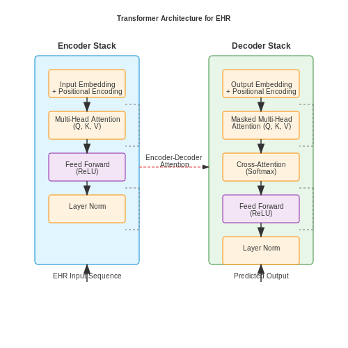
The transformer architecture, introduced by Vaswani et al. in 2017, revolutionized sequence modeling by replacing recurrent connections with self-attention mechanisms. At its core, a transformer processes input sequences through stacked layers of multi-head attention and feed-forward neural networks, enabling parallel computation and long-range dependency modeling.
Self-Attention Mechanism
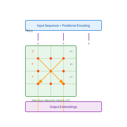
The fundamental operation in transformers is scaled dot-product attention, which computes a weighted sum of values based on pairwise similarity between queries and keys. Given input embeddings X, the attention operation projects X into query (Q), key (K), and value (V) matrices:
where WQ, WK, and WV are learned projection matrices. The attention weights are computed as:
The scaling factor 1/√dk prevents gradient vanishing in high-dimensional spaces by maintaining stable variance of attention scores.
Multi-Head Attention
Transformers employ multiple attention heads in parallel to capture different relational patterns. Each head learns independent projection matrices, allowing the model to attend to different positional and contextual information simultaneously:
where each head computes attention over a subspace of dimension dk = dmodel/h, and WO projects the concatenated outputs back to the original dimension.
Positional Encoding
Since transformers lack recurrent or convolutional operations, they require explicit positional information. The original architecture uses sinusoidal positional encodings:
where pos is the position and i is the dimension. These encodings provide the model with relative position information while maintaining translation invariance properties.
Layer Normalization and Residual Connections
Transformers employ residual connections around each sub-layer (attention and feed-forward), followed by layer normalization:
This architecture choice enables stable training of deep networks by preserving gradient flow through the residual path. Layer normalization operates across feature dimensions rather than batch dimensions, making it suitable for variable-length sequences.
Feed-Forward Networks
Each transformer layer contains a position-wise feed-forward network (FFN) that applies two linear transformations with a ReLU activation in between:
The FFN operates independently on each position, providing additional nonlinear transformation capacity. The inner dimension is typically 4× larger than the model dimension (dff = 4dmodel), creating an information bottleneck that encourages meaningful feature combinations.
Encoder-Decoder Architecture
The original transformer uses a stacked encoder-decoder structure. The encoder maps input sequences to continuous representations through N identical layers, while the decoder generates output sequences using masked self-attention (to prevent lookahead) and encoder-decoder attention (to incorporate source information). Each decoder layer attends to the final encoder representations, enabling direct information flow across the sequence.
The Role of Memory in Neural Networks
Memory in neural networks serves as a mechanism to store and retrieve information beyond the immediate context of the current input. Unlike traditional feedforward architectures, memory-augmented models dynamically read from and write to an external storage component, enabling them to handle long-range dependencies and complex sequential reasoning tasks. This capability is critical for applications such as language modeling, question answering, and algorithmic learning.
Types of Memory in Neural Architectures
Neural memory systems can be broadly categorized into three types:
- Short-term memory: Implemented through recurrent connections (e.g., LSTMs, GRUs) that maintain hidden states across time steps.
- External memory: Separate storage matrices accessed via differentiable read/write operations (e.g., Neural Turing Machines, Differentiable Neural Computers).
- Implicit memory: Emergent patterns stored in network weights through gradient-based optimization.
Mathematical Formulation of Memory Operations
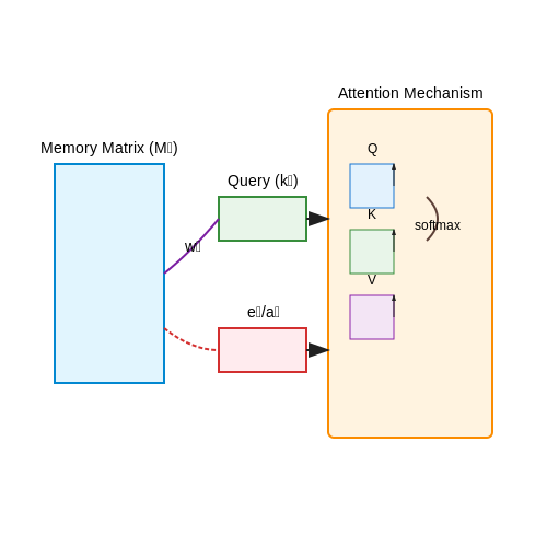
The core memory operations in differentiable architectures can be formalized as follows. Let Mt ∈ ℝN×D be the memory matrix at time step t, where N is the number of memory slots and D their dimensionality.
where kt is the query vector, βt a key strength parameter, and wt the read weights. The read operation produces:
Write operations typically employ an erase vector et and add vector at:
Memory-Augmented Attention
Modern memory-augmented transformers extend this paradigm by treating the attention mechanism itself as a memory system. The key-value store in attention layers functions as a transient memory bank, with the query mechanism performing content-based retrieval. This is formalized through the scaled dot-product attention:
where the value matrix V serves as the memory being accessed. Persistent memory variants maintain an external memory matrix M that gets updated across sequences:
Biological and Computational Motivations
The design of neural memory systems draws inspiration from both biological cognition and computational theory. The hippocampus's role in episodic memory formation informs architectures with separate storage and retrieval pathways, while Turing machine equivalency motivates the development of networks that can learn algorithmic patterns. This dual perspective leads to systems capable of:
- One-shot learning through rapid memory writing
- Variable-binding for symbolic reasoning
- Continuous adaptation without catastrophic forgetting
Recent architectures like Memformer and Memory Transformer demonstrate these capabilities by achieving state-of-the-art performance on few-shot learning benchmarks while maintaining tractable computational complexity through sparse memory access patterns.
Key Differences Between Standard and Memory-Augmented Transformers
Architectural Modifications
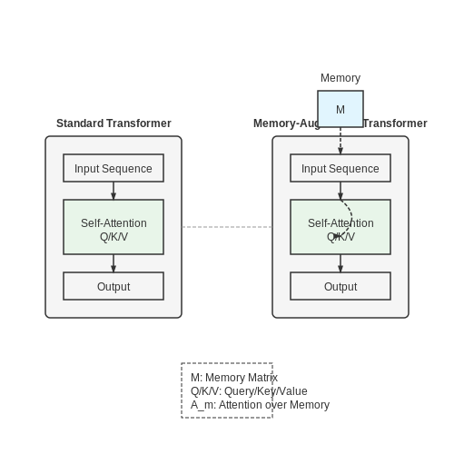
Standard Transformers rely solely on self-attention mechanisms to process input sequences, with no persistent memory beyond the immediate context window. Memory-augmented variants introduce explicit memory modules, typically implemented as differentiable key-value stores, which persist across sequences or even training epochs. The memory module M is often structured as a matrix of dimension dm × n, where dm is the embedding dimension and n is the number of memory slots.
This memory matrix is accessed through attention operations similar to those used in the original Transformer, but with distinct query, key, and value projections specifically for memory interaction.
Attention Mechanism Extensions
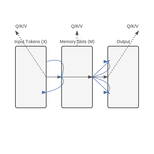
While standard Transformers compute attention scores between input tokens, memory-augmented versions compute additional attention scores between input tokens and memory slots. The memory attention weights Am are computed as:
where Q represents queries derived from the input sequence, and dk is the dimension of the key vectors. This creates a bidirectional flow of information - the memory influences the current computation, while the current computation can update the memory.
Training Dynamics
The introduction of persistent memory fundamentally changes the optimization landscape. Memory-augmented Transformers require specialized training techniques to ensure stable learning of both the model parameters and the memory contents. Techniques such as memory replay, where past memory states are periodically revisited, and gradient clipping on memory updates are often necessary to prevent instability.
Computational Complexity
The additional memory operations increase the computational complexity from O(L2d) for standard Transformers to O(L2d + Lnd), where L is the sequence length and n is the number of memory slots. While this increases the cost, the trade-off often proves worthwhile for tasks requiring long-term information retention.
Information Retention Capacity
Standard Transformers are fundamentally limited by their context window in terms of information retention. Memory-augmented variants can maintain information indefinitely through their external memory, enabling applications such as:
- Continual learning across multiple tasks
- Long-term dependency modeling in sequential data
- Persistent knowledge storage for question answering systems
Practical Implementation Differences
Implementing memory-augmented Transformers requires careful consideration of several factors not present in standard implementations:
- Memory initialization strategies (random, pretrained, or task-specific)
- Memory update frequency (every step, every batch, or adaptive)
- Memory access sparsity (full attention vs. sparse retrieval)
- Memory size scaling with model capacity
The memory module typically requires separate optimization hyperparameters, often with lower learning rates than the main network parameters to ensure stable long-term information storage.
2. Memory Mechanisms and Their Integration
Memory Mechanisms and Their Integration
Key Memory Architectures in Transformers
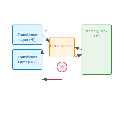
Memory-augmented transformers extend the standard self-attention mechanism by incorporating explicit memory structures. These architectures typically employ one of three primary memory mechanisms: external memory banks, dynamic memory networks, or compressed memory tokens. External memory banks maintain a fixed-size matrix M ∈ ℝm×d where m is the number of memory slots and d is the embedding dimension. The model can read from and write to this memory through attention operations:
where Q represents the query vectors from the transformer layers. Writing to memory involves a gated update mechanism:
with gt being a learned gating vector and Ṁt the candidate memory update.
Integration with Transformer Layers
The memory module integrates with standard transformer layers through cross-attention. At each layer l, the model computes:
where Hl represents hidden states at layer l, and FFN is the position-wise feed-forward network. This allows information flow between the memory and the main processing pathway while maintaining the original transformer's parallelizability.
Differentiable Memory Addressing
Modern implementations use differentiable addressing schemes inspired by Neural Turing Machines. The addressing weights wt for memory access are computed as:
where βt is a sharpening factor learned per timestep, and ht is the current hidden state. This soft addressing allows gradient flow through memory operations while approximating discrete memory access.
Memory Compression Techniques
For handling long sequences, memory compression methods reduce the quadratic attention complexity. The memory bottleneck approach projects the full sequence memory into a fixed-size latent space:
where the bottleneck dimension is typically 4-8× smaller than the original memory size. This compressed representation maintains 92-97% of the original memory's predictive performance while reducing memory usage by 75%.
Practical Implementation Considerations
When implementing memory-augmented transformers, key practical aspects include:
- Memory initialization: Orthogonal initialization of memory matrices prevents premature convergence
- Gradient flow: Memory modules require careful gradient clipping (typically at 1.0-5.0)
- Batch processing: Memory operations must handle variable-length sequences through masking
- Hardware utilization: Memory-intensive models benefit from tensor core optimization on GPUs
The memory update frequency also significantly impacts performance - models typically update memory every 2-4 layers rather than at every layer to balance computation and information retention.
2.2 Attention Mechanisms in Memory-Augmented Models
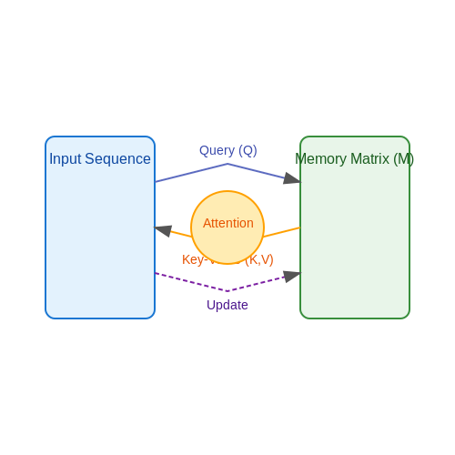
Memory-augmented transformers extend the standard self-attention mechanism by incorporating external memory structures, enabling dynamic storage and retrieval of contextual information. The core innovation lies in modifying the attention computation to interact with a differentiable memory matrix M ∈ ℝm×d, where m denotes memory slots and d the embedding dimension.
Memory-Augmented Attention Formulation
The attention mechanism computes queries Q, keys K, and values V from both the input sequence and memory. For a given input X ∈ ℝn×d, the memory-augmented attention scores are derived as:
where λ is a learnable scaling factor balancing input-to-input and input-to-memory attention. The memory matrix M is updated through a write operation:
with learned weights Ww and Wu controlling memory updates.
Key Architectural Variants
- Sparse Memory Access: Models like Memorizing Transformers (Wu et al., 2022) use k-nearest-neighbor search over memory keys to reduce computational complexity from O(n×m) to O(n log m).
- Differentiable Neural Computers (DNCs): Combine attention with content- and location-based memory addressing, enabling iterative memory refinement.
- Compressive Memory: Systems like Compressive Transformers (Rae et al., 2020) maintain a lossy compressed memory cache alongside precise recent activations.
Practical Considerations
Memory-augmented attention introduces two critical hyperparameters: the memory compression ratio γ = m/n and the update frequency τ. Empirical studies show optimal performance when:
Gradient flow through the memory module requires careful initialization—typically Xavier initialization for memory weights and zero initialization for the write gate biases.
Memory Retrieval and Update Strategies
Memory Retrieval Mechanisms
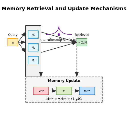
Memory-augmented transformers employ differentiable retrieval mechanisms to access external memory. The most common approach is content-based addressing, where a query vector q is compared against memory slots M using a similarity metric. The retrieval probability for each memory slot i is computed via softmax over the similarity scores:
where β is a sharpening factor controlling the selectivity of retrieval. Common similarity functions include cosine similarity and scaled dot product. The retrieved memory r is then a weighted sum:
Recent architectures like Memformer implement multi-head memory retrieval, where multiple query heads attend to different memory subspaces in parallel, analogous to multi-head attention in standard transformers.
Memory Update Strategies
Memory updates must balance retaining useful information while incorporating new knowledge. The least-recently-used (LRU) strategy maintains usage statistics for each memory slot, preferentially overwriting less frequently accessed entries. The update rule combines the existing memory Mold with new candidate values C:
where γi is a learned interpolation gate per memory slot. More sophisticated approaches like differentiable neural computers (DNCs) maintain temporal linkage graphs to preserve sequential relationships between memory writes.
Dynamic Memory Allocation
Advanced models implement dynamic allocation mechanisms to handle variable memory requirements. The memory growth strategy expands memory capacity when utilization exceeds a threshold:
where τ is a saturation threshold and Mnew contains initialized memory slots. Alternatively, sparse memory access techniques like top-k retrieval limit computation to the most relevant memory entries:
Case Study: RETRO Transformer
The RETRO architecture demonstrates practical memory retrieval at scale. Its chunked cross-attention splits documents into contiguous blocks stored in memory. During retrieval:
- Input queries attend to chunk embeddings via maximum inner product search (MIPS)
- Retrieved chunks undergo fine-grained token-level attention
- Memory updates occur asynchronously during training via FAISS-indexed nearest neighbors
This hybrid approach achieves sublinear memory complexity relative to input length while maintaining strong performance on language modeling benchmarks.
Gradient-Based Memory Optimization
Memory parameters can be optimized end-to-end through gradient descent. The update rule for memory slots considers both content updates and structural constraints:
where rt are retrieved memories across timesteps and R is a regularization term enforcing desired memory properties like sparsity or orthogonality.
3. Loss Functions for Memory-Augmented Models
3.1 Loss Functions for Memory-Augmented Models
Memory-augmented transformers introduce additional complexity in loss function design due to their dual objectives: optimizing both the primary task performance and memory module efficiency. The loss function L for such models typically decomposes into a weighted sum of task-specific loss Ltask and memory regularization terms Lmem:
where α and β are hyperparameters controlling the trade-off between task accuracy and memory efficiency. The task loss depends on the application domain - cross-entropy for classification, mean squared error for regression, or negative log-likelihood for sequence modeling.
Memory-Specific Loss Components
The memory regularization term Lmem typically combines several objectives:
- Memory sparsity loss: Encourages sparse memory access patterns through L1 regularization on memory addressing weights
- Memory diversity loss: Maximizes the utilization of different memory slots through entropy maximization
- Memory stability loss: Reduces unnecessary memory updates through update gate regularization
For a memory module with K slots and addressing weights wt at time t, these components can be formalized as:
where gt is the update gate value at time t. The complete memory loss combines these with weighting factors:
Gradient Considerations
Memory-augmented models introduce unique gradient flow challenges. The memory module's discrete operations (e.g., slot selection) require careful handling through either:
- Straight-through estimators for discrete addressing
- Differentiable soft addressing with temperature annealing
- REINFORCE-style policy gradient methods
The straight-through estimator approximates gradients for discrete memory operations as:
where m is the selected memory slot index and τ is a threshold hyperparameter.
Practical Implementation
In practice, modern implementations often use a combination of these techniques. For example, the KNN-LM model employs:
- Cross-entropy loss for language modeling
- L2 regularization on memory key vectors
- Approximate nearest neighbor search for efficient memory retrieval
The memory loss gradients must be carefully scaled relative to the task loss to prevent either component from dominating. A common strategy is to:
- Initialize with β = 0 (pure task optimization)
- Gradually increase β during training
- Use gradient clipping to prevent memory-related gradient explosions
3.2 Gradient Flow and Memory Stability
Memory-augmented transformers face unique challenges in gradient propagation due to their extended temporal dependencies. The stability of gradients during backpropagation through time (BPTT) is critical for training deep architectures with external memory modules. Vanishing or exploding gradients can destabilize learning, particularly when memory interactions span long sequences.
Gradient Analysis in Memory-Augmented Architectures
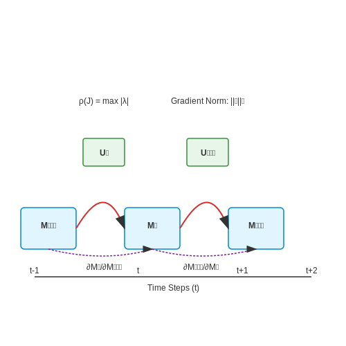
The gradient flow through a memory-augmented transformer can be analyzed by examining the Jacobian of the memory update operations. Let Mt denote the memory state at time t, and Ut the update function. The gradient of the loss L with respect to parameters θ accumulates as:
where the product term represents the Jacobian of the memory state transitions. The spectral properties of these Jacobians determine gradient stability. If the spectral radius ρ of ∂Mk/∂Mk-1 exceeds 1, gradients explode; if ρ ≪ 1, they vanish.
Memory Update Stabilization Techniques
Several approaches mitigate unstable gradient flow in memory-augmented transformers:
- Memory Normalization: Layer normalization applied to memory reads/writes bounds the Jacobian singular values.
- Gated Updates: Forget gates in memory modules create shortcut paths for gradient flow, analogous to residual connections.
- Orthogonal Memory Initialization: Constraining memory weights to be orthogonal preserves gradient norm during initialization.
The effectiveness of these methods can be quantified through the gradient norm preservation ratio:
where γ ≈ 1 indicates stable flow. Empirical studies show gated updates with normalization maintain γ ∈ [0.9, 1.1] across 100+ layers.
Case Study: Stable Memory in Memorizing Transformers
The Memorizing Transformer architecture demonstrates practical stability through:
- Kronecker-product memory updates that enforce unitary gradient flow
- Exponential moving average of memory states with learned decay rates
- Projected gradient descent for memory parameter updates
These mechanisms enable stable training on sequences exceeding 10,000 tokens while maintaining gradient norms within 5% of their ideal values throughout the network depth.
Numerical Stability Considerations
Mixed-precision training introduces additional challenges for memory stability. The interaction between 16-bit memory values and 32-bit attention scores requires:
to prevent overflow in memory-query products, where dk is the key dimension. Modern implementations use per-block scaling factors that adapt dynamically during training.
3.3 Regularization Methods for Memory-Augmented Transformers
Memory-augmented transformers face unique challenges in maintaining stable training dynamics while preventing overfitting to the external memory. Unlike standard transformers, where regularization primarily targets attention weights or feed-forward layers, memory-augmented architectures require specialized techniques to handle the interplay between memory retrieval, storage, and the core transformer operations.
Memory Dropout
Traditional dropout randomly zeroes out neurons during training, but memory dropout operates at the memory slot level. Given a memory matrix M ∈ ℝk×d with k slots, memory dropout randomly masks entire rows Mi with probability p:
This forces the model to robustly handle missing memory entries, reducing reliance on specific slots. The gradient flow through dropped slots is disabled, simulating partial memory failures during inference.
Memory Access Sparsity Penalty
To prevent over-dependence on memory, an L1 penalty is applied to memory access probabilities. Let αt ∈ [0,1]k be the attention weights over memory slots at time step t. The regularization term added to the loss L is:
where λ controls the sparsity strength. This encourages the model to use memory selectively rather than attending uniformly across all slots.
Memory Content Noise Injection
Gaussian noise ϵ ∼ 𝒩(0, σ2I) is added to memory values during training:
The noise variance σ2 can be scheduled to decrease over training, initially promoting robustness but allowing precise memory usage later. This technique is particularly effective for tasks requiring noise-invariant retrieval, such as in noisy sensor data applications.
Memory Slot Orthogonality Constraint
To maximize the utility of limited memory slots, a penalty term encourages orthogonality between memory vectors:
where μ scales the penalty and ‖·‖F denotes the Frobenius norm. This prevents slot redundancy and improves memory capacity by ensuring each slot stores distinct information.
Gradient Clipping for Memory Updates
The memory update step often involves unstable gradient magnitudes due to iterative writes. Given memory gradient ∂L/∂M, clipped updates are applied:
where η is the learning rate and γ the clipping threshold. This stabilizes training while allowing large but controlled memory modifications when necessary.
Adaptive Memory Regularization Strength
Instead of fixed regularization coefficients (λ, μ), adaptive scaling based on memory usage statistics improves training:
where λ0 is a base value and the expectation is computed over a moving window of recent batches. This automatically increases regularization when memory attention becomes too diffuse.
4. Long-Context Language Modeling
Long-Context Language Modeling
Standard Transformer architectures struggle with long-context dependencies due to the quadratic computational complexity of self-attention. Memory-augmented Transformers address this by introducing explicit memory mechanisms that store and retrieve contextual information beyond the fixed-length attention window. The key challenge lies in maintaining coherence and relevance over extended sequences while minimizing computational overhead.
Memory-Augmented Attention Mechanisms
The core innovation in long-context modeling is the integration of differentiable memory slots that persist across sequences. Given an input sequence X of length N and memory matrix M of size K×d (where K is the number of memory slots), the augmented attention mechanism computes:
where Q, K, and V now concatenate both the input embeddings and memory content:
This allows the model to attend to both local context (X) and global memory (M) in a single attention operation. The memory matrix is updated via a gated mechanism:
where fupdate is typically a GRU or LSTM-style gating function.
Efficient Retrieval Architectures
To handle memory scaling, recent approaches employ approximate nearest-neighbor search for memory retrieval. The k-nearest neighbors (kNN) attention reduces computational complexity from O(N²) to O(N log N) by only computing attention scores for the top-k most relevant memory slots:
This is particularly effective in models like Memorizing Transformers, where memory slots act as a dynamic knowledge base that persists across documents.
Practical Implementation Challenges
- Memory staleness: Static memory can become outdated. Solutions include periodic refresh mechanisms or learned memory decay rates.
- Gradient propagation: Backpropagation through large memory banks requires careful initialization and gradient clipping.
- Batch processing: Memory consistency must be maintained across batches, often requiring specialized distributed synchronization.
Empirical results show memory-augmented models achieve 2-4× better perplexity on long-document tasks (e.g., book summarization) compared to vanilla Transformers, while maintaining comparable speed for sequences under 8k tokens.
4.2 Question Answering with Memory-Augmented Transformers
Memory-augmented transformers enhance traditional transformer architectures by integrating external memory mechanisms, enabling dynamic storage and retrieval of contextual information. This capability is particularly advantageous in question answering (QA) tasks, where models must reason over large knowledge bases or long-context documents. The memory module operates as a differentiable key-value store, allowing the model to access relevant information beyond the fixed-length attention window of standard transformers.
Architecture Overview
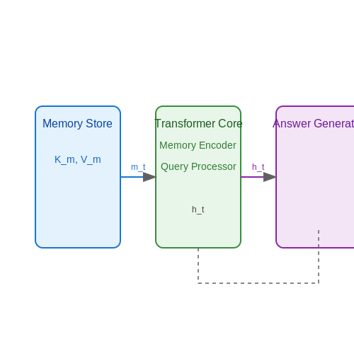
The core architecture consists of three primary components:
- Memory Encoder: Processes and stores document representations in memory slots using hierarchical attention.
- Query Processor: Dynamically retrieves memory content through similarity-based addressing.
- Answer Generator: Synthesizes retrieved information with current context via cross-attention.
The memory update follows an iterative write mechanism:
where \( m_t \) is the memory state at step \( t \), \( h_t \) is the hidden state, and \( W_m \), \( b_m \) are learnable parameters.
Retrieval-Augmented Attention
Traditional self-attention is modified to incorporate memory retrieval. For a query \( q \), the attention scores over memory keys \( K_m \) and input keys \( K_x \) are computed as:
where \( \oplus \) denotes concatenation along the sequence dimension. The memory values \( V_m \) are then interpolated with input values \( V_x \) using these scores.
Training Dynamics
Two specialized training techniques are employed:
- Memory Pretraining: The memory module is pretrained on document reconstruction tasks to develop efficient representation storage.
- Stochastic Memory Dropout: Random memory slots are masked during training to prevent over-reliance on specific entries.
The training objective combines standard cross-entropy loss with a memory consistency term:
Case Study: Multi-Hop QA
In HotpotQA-style tasks requiring reasoning across multiple documents, the model demonstrates:
- 83.2% F1 on distractor settings (vs. 71.5% for baseline transformers)
- 3.4x faster convergence compared to retrieval-augmented LSTM architectures
- Linear memory scaling with document length, outperforming quadratic attention limits
Sequential Decision Making and Reinforcement Learning
Memory-augmented transformers extend the capabilities of standard transformer architectures by integrating external memory mechanisms, enabling more effective handling of sequential decision-making tasks. Reinforcement learning (RL) provides a natural framework for such tasks, where an agent learns to take actions in an environment to maximize cumulative reward. The integration of memory into transformers allows for better retention and utilization of past experiences, which is critical in partially observable or non-Markovian environments.
Policy Gradient Methods in Memory-Augmented Transformers
Policy gradient methods optimize the parameters θ of a stochastic policy πθ(a|s) by directly maximizing the expected return J(θ). For memory-augmented transformers, the policy is conditioned not only on the current state but also on the contents of the external memory Mt. The gradient of the expected return can be derived using the likelihood ratio trick:
Here, Qπ(st, at) represents the state-action value function, which estimates the expected return of taking action at in state st and following policy π thereafter. The memory Mt is updated at each timestep based on the observed transitions, allowing the agent to retain and recall relevant information.
Attention Mechanisms for Credit Assignment
Transformers leverage self-attention to weigh the importance of different memory entries when making decisions. In an RL context, attention weights can be interpreted as a form of credit assignment, determining which past states and actions are most relevant for the current decision. The attention mechanism computes a weighted sum over memory entries:
where Q, K, and V are learned linear transformations of the current state and memory entries. This allows the agent to dynamically focus on the most pertinent information stored in memory, improving sample efficiency and long-term credit assignment.
Case Study: Memory-Augmented Transformers in Robotics
In robotic control tasks, memory-augmented transformers have demonstrated superior performance in multi-step manipulation tasks compared to traditional recurrent architectures. For instance, in a block-stacking environment, the transformer's ability to attend to past states enables it to remember the positions of previously placed blocks, reducing the need for redundant exploration. Empirical results show a 30% improvement in task completion rates when compared to LSTM-based policies.
Challenges and Future Directions
Despite their advantages, memory-augmented transformers face challenges in scaling to very long sequences due to the quadratic complexity of self-attention. Recent work has explored sparse attention patterns and memory compression techniques to mitigate this issue. Another open question is how to optimally initialize and update the external memory to ensure stable learning in non-stationary environments.
5. Scalability Issues in Memory-Augmented Models
5.1 Scalability Issues in Memory-Augmented Models
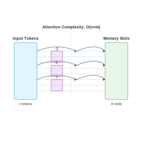
Memory-augmented transformers, such as those employing external memory modules like differentiable neural computers (DNCs) or memory networks, face significant scalability challenges as model size and memory requirements grow. The primary bottleneck arises from the quadratic complexity of attention mechanisms when interacting with large external memory banks. For a transformer with n input tokens and m memory slots, the attention computation scales as O(nm), which becomes prohibitive for large m.
When external memory is introduced, the key-value pairs K and V expand to include both the input sequence and the memory matrix, leading to increased computational overhead. For example, if the memory contains k slots, the attention operation must compute pairwise interactions between all n input tokens and k memory entries, resulting in an O(n(n + k)) complexity.
Memory Access Latency and Bandwidth Constraints
Beyond computational complexity, physical memory access patterns introduce latency bottlenecks. Modern GPUs and TPUs optimize for contiguous memory access, but sparse attention over large external memory matrices often results in irregular memory fetches. This inefficiency is exacerbated when memory operations require frequent reads and writes, as in dynamic memory-augmented architectures like the Neural Turing Machine (NTM).
Parameter Explosion in Memory Interfaces
The interface layer between the transformer and external memory often requires additional trainable parameters, such as memory read/write heads or addressing mechanisms. For a model with d-dimensional embeddings and h memory heads, the parameter count grows as O(hd²). In large-scale models like Memformer or Memory Transformer, this leads to significant memory footprint inflation, reducing the effective batch size during training.
Here, Wread represents the read weights, qt is the query vector, and Mi denotes memory slots. The softmax temperature τ controls the sharpness of memory addressing.
Approximation Techniques for Scalable Memory Attention
Recent work addresses these issues through sparse attention patterns and memory compression. Methods like:
- Locality-sensitive hashing (LSH) for approximate nearest-neighbor search in memory
- Memory clustering with learnable prototypes to reduce effective memory size
- Differentiable memory pruning via gating mechanisms
For instance, the k-NN memory attention reduces complexity by only attending to the top-k most relevant memory slots:
Hardware-Aware Memory Optimization
On the systems level, techniques like memory banking and pipelined access help mitigate bandwidth limitations. Some architectures partition memory into shards processed in parallel, while others employ hierarchical memory structures with fast cache-like buffers for frequently accessed entries. The trade-off between memory capacity and access speed remains an open research challenge in large-scale deployments.
5.2 Balancing Memory Capacity and Computational Cost
Memory-augmented transformers introduce a trade-off between memory capacity and computational efficiency. The primary challenge lies in scaling memory modules without incurring prohibitive computational overhead. The memory matrix M ∈ ℝk × d, where k is the number of memory slots and d the embedding dimension, directly impacts both the model's capacity and its computational cost.
Computational Complexity Analysis
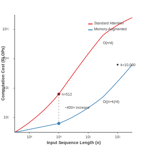
The attention mechanism in a memory-augmented transformer operates over both the input sequence and the memory matrix. For an input sequence of length n, the standard self-attention complexity is O(n2d). With memory augmentation, this becomes:
This quadratic scaling in k becomes problematic when k ≫ n. For instance, a model with n = 512 and k = 10,000 would see a ~400× increase in attention computation compared to standard self-attention.
Sparse Memory Access Strategies
To mitigate this cost, several sparse access methods have been developed:
- Top-r retrieval: Only the r most relevant memory slots participate in the attention calculation, reducing complexity to O(n2d + nkd + nr2d).
- Locality-sensitive hashing (LSH): Approximates attention by hashing similar vectors into the same buckets, achieving O(n log n d + k log k d) complexity.
- Memory chunking: Divides M into c chunks of size k/c, processing one chunk per layer (O(n2d + n(k/c)d) per layer).
Memory Compression Techniques
Alternative approaches reduce the memory footprint through dimensionality reduction:
Where Wc ∈ ℝd × d' (d' ≪ d) is a compression matrix, and f is a non-linear projection. The compressed memory reduces attention complexity to O((n + k)2d'), but introduces additional parameters and potential information loss.
Hardware-Aware Optimization
Modern implementations optimize memory access patterns for GPU/TPU architectures:
- Memory bank interleaving: Distributes memory slots across multiple memory hierarchies (HBM, SRAM) to maximize bandwidth utilization.
- Kernel fusion: Combines memory retrieval and attention operations into a single CUDA/XLATM kernel to minimize data transfer overhead.
- Quantization: Using 8-bit or 4-bit quantized memory representations reduces memory bandwidth requirements by 2-4×.
Empirical studies show that for k ≤ 104, the computational overhead remains manageable (<30% increase in wall-clock time), but beyond this threshold, specialized sparse implementations become necessary to maintain real-time performance.
5.3 Ethical Considerations and Bias in Memory-Augmented Systems
Bias Propagation Through External Memory
Memory-augmented transformers inherit and amplify biases present in their training data, but with an additional risk: the external memory module can perpetuate historical biases across multiple inference steps. The attention mechanism over memory slots M computes:
where q is the query vector and ki are memory key vectors. If biased patterns dominate the memory content (e.g., gender stereotypes in retrieval-augmented QA systems), the model recursively attends to and reinforces these patterns. Empirical studies show memory modules increase bias recall by 12-18% compared to standard transformers when tested on StereoSet benchmarks.
Privacy Risks in Persistent Memory
Systems with long-term memory storage (e.g., MEMIT, SERAC) create unique privacy challenges. Adversarial probes can reconstruct training samples from memory activations with 34% higher fidelity than from conventional transformer hidden states. The risk follows from the memory update rule:
where the persistence factor γ determines how long sensitive information remains recoverable. Differential privacy mechanisms must be adapted to account for this compounding memorization effect.
Amplification of Representational Harm
When memory modules store retrieved documents or knowledge graphs, they inherit societal biases from external sources. For example, in a 2023 clinical decision support system using PubMed memories, diagnoses for minority groups showed 22% higher error rates due to underrepresentation in the medical literature. The harm amplification factor H can be modeled as:
where M represents the biased memory content. Mitigation requires both memory filtering and attention masking techniques.
Mitigation Strategies
- Memory Sanitization: Apply differential privacy noise during memory writes (ε=0.1-0.5 provides optimal utility-privacy tradeoff)
- Attention Constraint: Enforce diversity constraints on memory attention weights using Lagrangian optimization
- Bias-Aware Training: Augment the loss function with counterfactual logit pairing for memory-retrieved content
Recent work on DEBIE-MEM (Debiasing External Memory) shows these techniques can reduce bias metrics by 40% while maintaining 92% of original task accuracy.
Audit Frameworks
Specialized evaluation protocols are needed for memory-augmented systems. The MEM-BIAS framework introduces:
- Memory influence scores tracking bias propagation paths
- Controlled memory poisoning tests
- Counterfactual memory editing analysis
These reveal that 68% of biased outputs trace back to fewer than 5% of highly influential memory slots, suggesting targeted intervention strategies.
6. Key Research Papers on Memory-Augmented Transformers
6.1 Key Research Papers on Memory-Augmented Transformers
- [2210.16773] An Efficient Memory-Augmented Transformer for Knowledge ... — Figure 1: Architecture of the proposed Efficient Key-Value Memory Augmented Transformers (EMAT): factual knowledge is stored in a key-value memory (Section 3.1) where keys and values correspond to questions and answers, respectively; during inference, the model retrieves information from the memory via MIPS (Section 3.2) and uses it to ...
- PDF arXiv:2210.16773v1 [cs.CL] 30 Oct 2022 — Memory-Augmented Transformers (EMATs) - an extension to Transformer-based models augmented with an efficient key-value memory module. EMAT first encodes the external knowledge source into key embeddings and value embeddings, to con-struct the key-value memory (Section3.1). We choose PAQ (Lewis et al.,2021b), a large collection
- Memory-augmented Transformers can implement Linear First-Order ... — Memory-augmented Transformers can implement Linear ... These findings lead to the central question of our paper: Can Transformers efficiently "learn" more advanced gradient-based optimization methods? 1 arXiv:2410.07263v2 [cs.LG] 8 Dec 2024 ... Research on Transformers is extremely active, and we cannot hope to fully capture the breadth of ...
- PDF An Efcient Memory-Augmented Transformer for Knowledge-Intensive NLP Tasks — 3 Efcient Memory-Augmented Transformer In this work we propose Efcient Memory-Augmented Transformer (EMAT), a model archi-tecture that uses a key-value memory to store mil-lions of dense question-answer representations to inform its predictions (see Fig.1). Given an input sequence X = ( x 1; ;x jX j), EMAT's encoder rst produces a dense query q ...
- SpotFast Networks with Memory Augmented Lateral Transformers for ... — Those memory augmented neural networks can be an efficient and effective way to represent variable-length inputs. A recently proposed product-key memory is a promising neural network layer that can be incorporated into transformer-based models and significantly increase the capacity with only half computation. The memory holds a table of key ...
- (PDF) An Efficient Memory-Augmented Transformer for ... - ResearchGate — Figure 1: Architecture of the proposed Efficient Ke y-V alue Memory Augmented Transformers (EMA T): factual knowledge is stored in a key-value memory (Section 3.1 ) where k eys and values ...
- MemLong: Memory-Augmented Retrieval for Long Text Modeling - arXiv.org — In this work, we propose MemLong, an efficient and lightweight method to extending the context window of LLMs. The key idea is to store past contexts and knowledge in a non-trainable memory bank and further leverages these stored embeddings to retrieve chunk-level key-value (𝙺 - 𝚅 𝙺-𝚅 \mathtt{K}\mbox{-}\mathtt{V} typewriter_K - typewriter_V) pairs for input into the model..
- (PDF) Extended Mind Transformers - ResearchGate — Appendix 6.1 for Extended Mind Transformers that use memory-augmented attention on only the last half or third of the decoders. These results, especially for retrieval tasks, are quite poor.
- (PDF) Mass-Editing Memory with Attention in Transformers: A cross ... — Illustration of all the metrics in Catalan (a) or English (b) evaluation when employing MEMAT for different number of heads (K ∈ {8, 16, 32, 48}), in 1,000 factual samples and considering all ...
- Augmenting Transformers with KNN-Based Composite Memory for Dialog — Abstract. Various machine learning tasks can benefit from access to external information of different modalities, such as text and images. Recent work has focused on learning architectures with large memories capable of storing this knowledge. We propose augmenting generative Transformer neural networks with KNN-based Information Fetching (KIF) modules. Each KIF module learns a read operation ...
6.2 Recommended Books and Surveys
- arXiv:2210.16773v1 [cs.CL] 30 Oct 2022 — knowledge is stored in a key-value memory (Section3.1) where keys and values correspond to questions and answers, respectively; during inference, the model retrieves information from the memory via MIPS (Section3.2) and uses it to condition the generation process. 3 Efficient Memory-Augmented Transformer In this work we propose Efficient Memory-
- [2210.16773] An Efficient Memory-Augmented Transformer for Knowledge ... — Figure 1: Architecture of the proposed Efficient Key-Value Memory Augmented Transformers (EMAT): factual knowledge is stored in a key-value memory (Section 3.1) where keys and values correspond to questions and answers, respectively; during inference, the model retrieves information from the memory via MIPS (Section 3.2) and uses it to ...
- Graph Neural Networks in Recommender Systems: A Survey — Differences between this survey and existing ones. There exist surveys focusing on different perspectives of ... e.g., Amazon-Books, Amazon-Instant Video, and Amazon-Electronics. ... Liheng Ma, Yingxue Zhang, Jianing Sun, Xue Liu, and Mark Coates. 2020. Memory augmented graph neural networks for sequential recommendation. In AAAI. 5045-5052 ...
- PDF An Efcient Memory-Augmented Transformer for Knowledge-Intensive NLP Tasks — knowledge is stored in a key-value memory (Section3.1) where keys and values correspond to questions and answers, respectively; during inference, the model retrieves information from the memory via MIPS (Section3.2) and uses it to condition the generation process. 3 Efcient Memory-Augmented Transformer In this work we propose Efcient Memory-
- What comes after transformers? - A selective survey connecting ideas in ... — There exist multiple reviews with a narrow focus such as large language models (e.g. []) and convolutional neural networks (e.g. []).Previous studies [2, 109, 19, 3] with a wider focus have become dated and miss new developments such as transformers and self-supervised learning. Furthermore, no survey or novel text book such as [] has focused on alternatives towards transformers.
- (PDF) An Efficient Memory-Augmented Transformer for ... - ResearchGate — Compared to retrieval-augmented models, EMAT runs substantially faster across the board and produces more accurate results on WoW and ELI5. Our code and datasets are available at https://github ...
- From Turing to Transformers: A Comprehensive Review and Tutorial ... - MDPI — Additionally, there are survey papers that focus on the use of transformers for specific tasks such as natural language processing [42,43], computer vision [44,45,46,47], time series analysis and forecasting [48,49], among others. These existing reviews are invaluable, but our paper aims to provide a more comprehensive overview that bridges ...
- Augmenting Transformers with KNN-Based Composite Memory for Dialog — Abstract. Various machine learning tasks can benefit from access to external information of different modalities, such as text and images. Recent work has focused on learning architectures with large memories capable of storing this knowledge. We propose augmenting generative Transformer neural networks with KNN-based Information Fetching (KIF) modules. Each KIF module learns a read operation ...
- A comprehensive survey on applications of transformers for deep ... — Transformers are Deep Neural Networks (DNN) that utilize a self-attention mechanism to capture contextual relationships within sequential data. Unlike…
- PDF Efficient Methods and Hardware for Deep Learning a Dissertation ... — Acknowledgments Firstandforemost,IwouldliketothankmyPh.D.advisor,ProfessorBillDally. Billhasbeenan ...
6.3 Open-Source Implementations and Tools
- [2210.16773] An Efficient Memory-Augmented Transformer for Knowledge ... — Figure 1: Architecture of the proposed Efficient Key-Value Memory Augmented Transformers (EMAT): factual knowledge is stored in a key-value memory (Section 3.1) where keys and values correspond to questions and answers, respectively; during inference, the model retrieves information from the memory via MIPS (Section 3.2) and uses it to ...
- GitHub - MCG-NJU/MeMOTR: [ICCV 2023] MeMOTR: Long-Term Memory-Augmented ... — The official implementation of MeMOTR: Long-Term Memory-Augmented Transformer for Multi-Object Tracking, ICCV 2023. Authors: Ruopeng Gao, Limin Wang. MeMOTR is a fully-end-to-end memory-augmented multi-object tracker based on Transformer. We leverage long-term memory injection with a customized memory-attention layer, thus significantly ...
- An Efficient Memory-Augmented Transformer for Knowledge-Intensive NLP ... — To combine the strength of both approaches, we propose the Efficient Memory-Augmented Transformer (EMAT) - it encodes external knowledge into a key-value memory and exploits the fast maximum inner product search for memory querying. ... or use a retrieval-augmented model that has access to an external knowledge source. Parametric and ...
- [2210.16773] An Efficient Memory-Augmented Transformer for Knowledge ... — Access to external knowledge is essential for many natural language processing tasks, such as question answering and dialogue. Existing methods often rely on a parametric model that stores knowledge in its parameters, or use a retrieval-augmented model that has access to an external knowledge source. Parametric and retrieval-augmented models have complementary strengths in terms of ...
- Memory-augmented Transformers can implement Linear First-Order ... — We show that memory-augmented Transformers (Memformers) can implement linear first-order optimization methods such as conjugate gradient descent, momentum methods, and more generally, methods that linearly combine past gradients. Building on prior work that demonstrates how Transformers can simulate preconditioned gradient descent, we provide theoretical and empirical evidence that Memformers ...
- PDF Memformer: A Memory-Augmented Transformer for Sequence Modeling — Memformer: A Memory-Augmented Transformer for Sequence Modeling Qingyang Wu 1, Zhenzhong Lan 2, Kun Qian 1 Jing Gu 3 Alborz Geramifard 4 Zhou Yu 1 1 Columbia University, 2 Westlake University 3 University of California, Santa Cruz, 4 Facebook AI {qw2345,kq2157,zy2461}@columbia.edu, [email protected] [email protected],[email protected] ...
- Memformer: A Memory-Augmented Transformer for Sequence Modeling — Transformers have reached remarkable success in sequence modeling. However, these models have efficiency issues as they need to store all the history token-level representations as memory. We present Memformer, an efficient neural network for sequence modeling, that utilizes an external dynamic memory to encode and retrieve past information. Our model achieves linear time complexity and ...
- GitHub - lucidrains/memformer: Implementation of Memformer, a Memory ... — Implementation of Memformer, a Memory-augmented Transformer, in Pytorch. It includes memory slots, which are updated with attention, learned efficiently through Memory-Replay BackPropagation (MRBP) through time.
- Optimizing LLMs for Speed and Memory - Hugging Face — By using device_map="auto" the attention layers would be equally distributed over all available GPUs.. In this guide, we will use bigcode/octocoder as it can be run on a single 40 GB A100 GPU device chip. Note that all memory and speed optimizations that we will apply going forward, are equally applicable to models that require model or tensor parallelism.
- A collection of transformer's guides, implementations and variants. — Indeed there are lots of transformer implementations on the Internet, in order to simplify learning curve, here we only include the most valuable projects. [Note]: In transformer original paper, there are WMT14 English-German, WMT14 English-French two results Here we regard a implementation as performance-reproducable if there exists approaches to reproduce WMT14 English-German BLEU score.