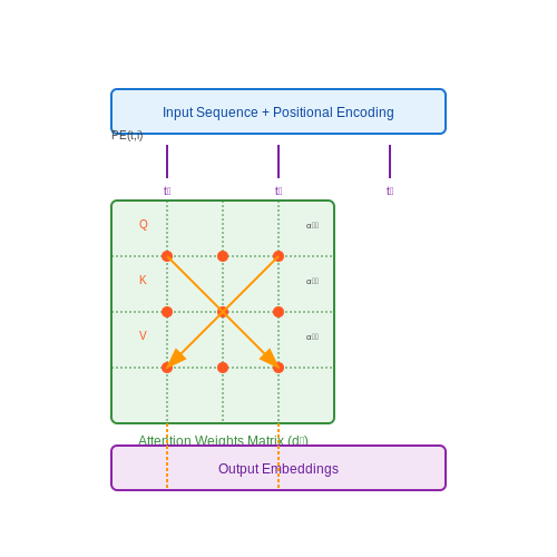
Positional Encoding in Transformers
1. The Need for Positional Encoding in Transformers
The Need for Positional Encoding in Transformers
Transformers rely entirely on self-attention mechanisms to process input sequences, unlike recurrent or convolutional architectures that inherently capture sequential or spatial relationships. While self-attention computes pairwise interactions between all tokens in parallel, it is permutation-invariant—reordering input tokens does not alter the output. This property poses a critical challenge for modeling sequential data, where positional information is semantically meaningful (e.g., word order in language or time steps in signals).
Mathematical Intuition Behind Permutation Invariance
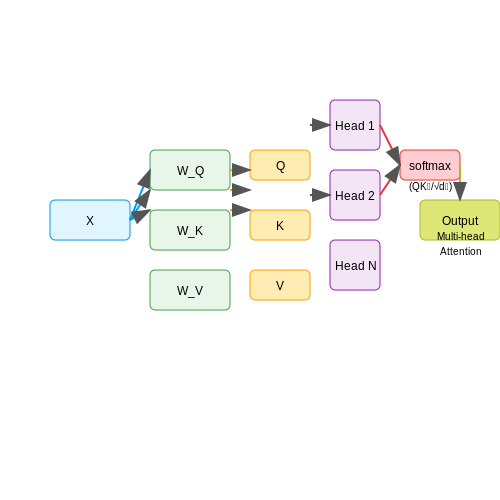
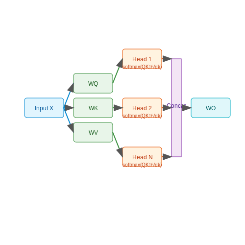
Given an input sequence X = (x1, x2, ..., xn), the self-attention operation computes a weighted sum of values V based on query-key compatibility:
Since the softmax operation is symmetric with respect to input permutations, shuffling the rows of X (and thus Q, K, V) leaves the output unchanged. For example, the sentences "The cat sat on the mat" and "Mat the on sat cat the" would produce identical representations without explicit positional cues.
Why Absolute Position Matters
In natural language processing, syntactic and semantic structures depend on token order:
- Grammaticality: "Dog bites man" ≠ "Man bites dog"
- Coreference resolution: Pronouns refer to earlier nouns ("She" depends on prior context)
- Temporal sequences: Time-series forecasting requires strict chronological ordering
Convolutional networks partially address this through local receptive fields, while RNNs encode position via sequential processing. Transformers, however, must explicitly inject positional information to avoid treating sequences as unordered sets.
Design Requirements for Positional Encoding
An effective positional encoding scheme must satisfy:
- Uniqueness: Each position has a distinct representation
- Boundedness: Encodings should not grow indefinitely with sequence length
- Generalization: The model should handle sequences longer than those seen during training
- Determinism: Positions must be consistently encoded across different inputs
Sinusoidal positional encodings, introduced in the original Transformer paper, meet these criteria by projecting positions onto continuous sinusoidal functions of varying frequencies:
where pos is the position index and i ranges over the embedding dimensions. This formulation allows the model to learn relative positions through linear transformations and naturally generalizes to unseen sequence lengths.
Practical Implications
Modern implementations often replace sinusoidal encodings with learned positional embeddings, which treat positions as discrete indices to be embedded. While both approaches perform comparably, learned embeddings may offer marginal gains on domain-specific tasks with fixed maximum sequence lengths. However, sinusoidal encodings remain theoretically appealing for their ability to extrapolate to arbitrary sequence lengths—a critical feature for applications like document summarization or genome processing.
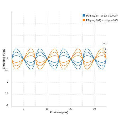
1.2 Key Properties of Effective Positional Encoding
Positional encoding in transformers must satisfy several critical properties to ensure the model can effectively learn and generalize sequential dependencies. These properties stem from the need to preserve relative and absolute positional information while maintaining stability during training.
1. Uniqueness
Each position in the sequence must have a distinct encoding to avoid ambiguity. For a sequence of length L, the positional encoding function PE: {1, 2, ..., L} → ℝd must be injective, where d is the embedding dimension. The sinusoidal encoding scheme proposed in the original transformer paper achieves this by assigning unique frequency-phase combinations to each position:
where pos is the position and i is the dimension index. The geometric progression of frequencies ensures uniqueness across positions.
2. Translation Invariance for Relative Positions
Effective positional encoding should enable the model to learn relative positions independently of absolute positions. The sinusoidal encoding satisfies this because the dot product between two position encodings depends only on their offset Δpos = pos2 - pos1:
where M(Δpos) is a linear transformation matrix. This property allows self-attention to generalize to unseen sequence lengths.
3. Boundedness and Stability
Positional encodings must remain within a stable numerical range to prevent gradient explosion or vanishing during training. The sinusoidal functions naturally bound the values to [-1, 1]. For learned positional embeddings, this requires careful initialization (typically with small random values) and sometimes normalization.
4. Directionality Awareness
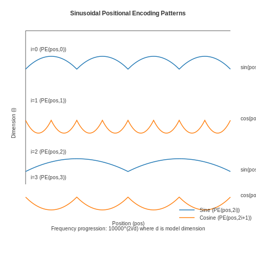
The encoding must preserve the order of positions. Sinusoidal encodings achieve this through the monotonicity of the wavelength progression - higher dimensions correspond to higher frequencies that change more rapidly with position. This creates a hierarchical representation where:
- Low-frequency components capture long-range dependencies
- High-frequency components encode fine-grained positional information
5. Generalization to Unseen Lengths
The encoding scheme should extrapolate to sequences longer than those seen during training. Analytical functions (like sinusoids) naturally satisfy this, while learned positional embeddings may struggle. The wavelength progression in sinusoidal encoding ensures that even for very large pos, the encoding values remain bounded and meaningful.
6. Efficient Computation
For practical deployment, positional encoding should be computationally efficient to generate. The sinusoidal encoding can be computed in O(1) time per position using closed-form expressions, unlike learned embeddings which require memory storage proportional to the maximum sequence length.
Recent variants like Rotary Position Embedding (RoPE) and Relative Position Biases maintain these properties while offering improved performance on certain tasks. RoPE, for instance, encodes relative position information directly into the attention mechanism through rotation matrices:
where RΔpos is a rotation matrix that depends only on the relative position Δpos = m - n.
1.3 Comparison with Recurrent and Convolutional Architectures
Transformers, unlike recurrent neural networks (RNNs) or convolutional neural networks (CNNs), rely entirely on self-attention mechanisms and positional encoding to process sequential data. This architectural shift eliminates several limitations inherent in RNNs and CNNs while introducing new computational trade-offs.
Recurrent Neural Networks (RNNs)
RNNs process sequences iteratively, maintaining a hidden state that propagates information through time. The recurrence relation for a simple RNN at time step t is:
where ht is the hidden state, xt the input, and σ an activation function. While theoretically capable of handling long-range dependencies, RNNs suffer from vanishing/exploding gradients in practice. Long Short-Term Memory (LSTM) and Gated Recurrent Unit (GRU) variants mitigate this but still process sequences sequentially, preventing parallelization.
Convolutional Neural Networks (CNNs)
CNNs apply sliding kernel operations across sequences, capturing local patterns through hierarchical feature extraction. For a 1D convolutional layer with kernel K of width w:
While CNNs allow parallel computation, their receptive fields grow linearly with depth. Dilated convolutions increase the effective window size but require careful architectural tuning. CNNs implicitly learn position-dependent patterns through kernel shifts, unlike Transformers where position information is explicitly injected.
Key Comparative Advantages of Transformers
- Parallelization: Self-attention computes all pairwise interactions simultaneously, whereas RNNs require sequential computation.
- Long-range dependencies: Attention heads directly model relationships between any positions, overcoming the limited receptive fields of CNNs and gradient issues in RNNs.
- Interpretability: Attention weights provide explicit interaction patterns, unlike the opaque state transitions in RNNs or CNN feature maps.
Computational Complexity Analysis
The asymptotic costs for sequence length n and embedding dimension d reveal critical trade-offs:
While Transformers dominate for moderate n, the quadratic O(n²) attention cost becomes prohibitive for very long sequences, motivating sparse attention variants.
Empirical Performance Characteristics
On the WMT 2014 English-German translation task, the original Transformer achieved a 28.4 BLEU score with 3.3× faster training than the best convolutional sequence model and 12× faster than recurrent architectures. The performance gap widens on tasks requiring very long-range reasoning, such as document-level summarization or program synthesis.
2. Sinusoidal Positional Encoding: Definition and Derivation
Sinusoidal Positional Encoding: Definition and Derivation
Sinusoidal positional encoding was introduced in the original Transformer paper (Attention Is All You Need, Vaswani et al., 2017) as a way to inject positional information into the input embeddings without requiring recurrence or convolution. The encoding is designed such that the model can easily learn to attend by relative positions, owing to the sinusoidal functions' linear relationships.
Mathematical Formulation
For a given position pos and dimension i, the positional encoding PE(pos, i) is defined as:
where dmodel is the embedding dimension. The wavelengths form a geometric progression from 2π to 10000·2π, allowing the model to capture both fine-grained and coarse-grained positional information.
Derivation and Intuition
The sinusoidal functions were chosen because they allow the model to learn relative positions through simple linear transformations. For a fixed offset k, PEpos+k can be represented as a linear function of PEpos, which is crucial for the self-attention mechanism to generalize to sequence lengths not seen during training.
To see why, consider the angle addition formulas:
where ωj = 1/100002j/dmodel. This shows that the positional encoding at pos + k can be expressed as a linear transformation of the encoding at pos, enabling the model to learn relative position patterns.
Properties and Advantages
- Uniqueness: Each position has a unique encoding due to the sinusoidal functions' periodicity and the geometric progression of wavelengths.
- Boundedness: The values are constrained to [-1, 1], preventing the embeddings from becoming too large.
- Generalization: The linear relationships allow the model to extrapolate to sequence lengths longer than those seen during training.
Implementation Considerations
In practice, the positional encodings are either added to or concatenated with the token embeddings. The original Transformer uses addition, which works well because the sinusoidal encodings and learned embeddings occupy similar value ranges. The choice of 10000 as the base for the geometric progression was empirically determined but can be tuned for specific applications.
For high-dimensional models, the sinusoidal encodings for different dimensions will cover a wide range of frequencies, allowing the model to capture both local and global positional relationships.
Intuition Behind the Sine and Cosine Functions
The choice of sinusoidal functions for positional encoding in transformers is not arbitrary—it stems from mathematical properties that enable the model to efficiently capture both absolute and relative positional information. The key insight is that sine and cosine functions exhibit periodicity and linear combinations that allow the model to learn positional relationships through simple linear transformations.
Mathematical Basis of Sinusoidal Encoding
The positional encoding for a position pos and dimension i is defined as:
where dmodel is the embedding dimension. The alternating sine and cosine pattern ensures that each position has a unique encoding while maintaining useful geometric properties.
Why Sine and Cosine Work
The sinusoidal functions were chosen because they satisfy three critical properties:
- Unique representation: Each position gets a distinct encoding vector
- Bounded values: Outputs are constrained to [-1, 1], preventing numerical instability
- Relative position awareness: The encoding of position pos + k can be represented as a linear function of the encoding at position pos
The last property is particularly important—it means the model can learn to attend to relative positions through simple linear transformations. This can be shown mathematically:
where Mk is a transformation matrix that depends only on the offset k. This linear relationship emerges from the trigonometric identity:
where ωi = 1/100002i/dmodel. These identities show that the encoding at pos + k can indeed be expressed as a linear combination of the encoding at pos.
Frequency Spectrum of Encodings
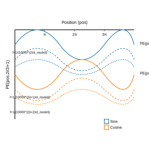
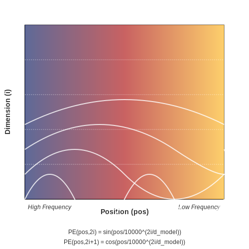
The frequencies in the positional encoding decrease exponentially across dimensions, creating a geometric progression from high to low frequencies. This multi-scale representation allows the model to simultaneously learn both local and global positional relationships:
The base 10000 was chosen empirically—smaller values would make the frequencies decay too quickly, while larger values would make them decay too slowly. This particular base provides a good balance across typical sequence lengths encountered in practice.
Visual Interpretation
When visualized, the positional encodings form a striped pattern where the frequency of oscillation decreases with increasing dimension. Lower dimensions (left side of the embedding) change rapidly across positions, capturing fine-grained positional information, while higher dimensions (right side) change slowly, capturing coarse-grained positional information.
2.3 Encoding Dimensionality and Frequency Bands
The choice of encoding dimensionality d in positional encoding critically impacts the model's ability to capture positional relationships. For a Transformer with embedding size d, the sinusoidal positional encoding assigns unique frequencies to each dimension, creating a structured pattern that allows the model to attend to relative or absolute positions.
Frequency Band Allocation
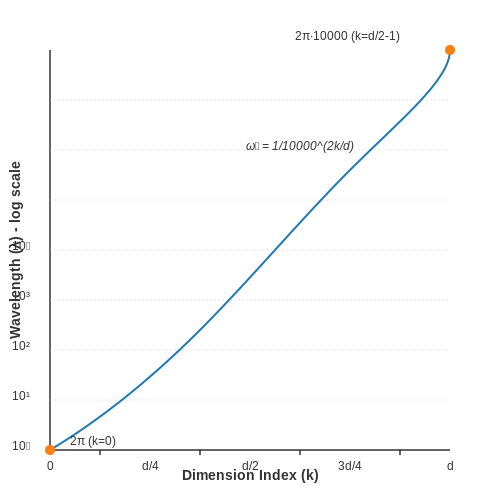
The frequency term ωk in the sinusoidal functions is not arbitrary but follows a geometric progression across dimensions. For dimension i, the wavelength forms a geometric sequence from 2π to 2π·10000, ensuring coverage across multiple scales:
where k ranges from 0 to d/2-1. This design creates a series of frequency bands where lower dimensions (small k) correspond to high-frequency variations, while higher dimensions capture low-frequency patterns. The logarithmic scaling ensures that the positional information is distributed evenly across the embedding space.
Dimensionality Effects
The choice of d affects two key properties:
- Maximum sequence length: The highest-frequency component (dimension 0) must have a wavelength shorter than the maximum sequence length to avoid aliasing.
- Positional resolution: Lower-frequency components (higher dimensions) provide coarser positional information, while higher frequencies give fine-grained distinctions.
For a model with d=512, the frequency bands range from wavelengths of ~6.28 (2π) to ~62,832 (2π·10000) positions. This allows the encoding to handle sequences up to tens of thousands of tokens while maintaining precise positional information for nearby tokens.
Interdimensional Relationships
The sinusoidal functions create orthogonal basis vectors across dimensions. For any fixed offset δ, the dot product between the positional encodings at positions pos and pos+δ depends only on δ, not on pos itself. This property emerges from the trigonometric identity:
The sum forms a kernel that decays smoothly with increasing δ, allowing the model to learn position-aware attention patterns. The frequency band structure ensures this kernel has rich spectral content across different distance scales.
Practical Considerations
In practice, several modifications to the original formulation have proven beneficial:
- Learned frequency scaling: Some implementations make the 10000 constant learnable, allowing the model to adjust its frequency bands.
- Dimension pruning: Higher dimensions (with wavelengths > maximum sequence length) can often be removed without performance loss.
- Mixed precision: The geometric progression helps maintain numerical stability when using lower-precision floating point formats.
The frequency band structure also explains why positional encodings generalize to sequences longer than those seen during training - the sinusoidal patterns naturally extend beyond the training distribution while maintaining their relative properties.
3. Learned Positional Embeddings
3.1 Learned Positional Embeddings
Unlike sinusoidal positional encoding, learned positional embeddings treat position information as a set of trainable parameters. These embeddings are initialized randomly and optimized during training, allowing the model to adaptively learn the most effective positional representations for the task at hand. This approach was first introduced in the original Transformer paper by Vaswani et al. (2017) and has since been widely adopted in variants like BERT and GPT.
Mathematical Formulation
Given a sequence of length L and an embedding dimension d, learned positional embeddings are represented as a matrix P ∈ ℝL×d. For a token at position pos in the sequence, its positional embedding is the pos-th row of P. The final input representation is obtained by summing the token embedding E and the positional embedding Ppos:
During training, P is updated via backpropagation alongside other model parameters. This allows the embeddings to capture complex positional patterns that may not be easily represented by fixed sinusoidal functions.
Advantages Over Sinusoidal Encoding
- Adaptability: Learned embeddings can adjust to the specific positional dependencies of the dataset, potentially capturing non-linear or hierarchical patterns.
- Simplicity: No need to manually design frequency bands or phase shifts as in sinusoidal encoding.
- Scalability: Can handle sequences longer than those seen during training by extrapolating or using techniques like relative positional embeddings.
Limitations and Challenges
Despite their flexibility, learned positional embeddings have notable drawbacks:
- Fixed maximum sequence length: The matrix P has a predefined size, limiting the model to sequences of length ≤ L.
- Lack of generalization: Unlike sinusoidal encoding, learned embeddings do not inherently generalize to unseen positions, making them less suitable for tasks requiring strong extrapolation.
- Training instability: Random initialization can sometimes lead to suboptimal convergence, especially for small datasets.
Practical Implementation
In modern implementations, learned positional embeddings are typically combined with token embeddings through addition. For example, in PyTorch:
import torch
import torch.nn as nn

class LearnedPositionalEmbedding(nn.Module):
    def __init__(self, max_seq_len, d_model):
        super().__init__()
        self.embedding = nn.Embedding(max_seq_len, d_model)

    def forward(self, x):
        positions = torch.arange(x.size(1), device=x.device
        return x + self.embedding(positions)
Some architectures, like BERT, also use learned segment embeddings to distinguish between different sequences (e.g., sentence pairs in next-sentence prediction).
Extensions and Variants
Recent work has proposed several enhancements to basic learned positional embeddings:
- Relative Positional Embeddings: Models like Transformer-XL and DeBERTa use learned embeddings that depend on the relative distance between tokens rather than absolute positions.
- Dynamic Positional Embeddings: Methods like DYPE adjust the embeddings based on input content, allowing position representations to vary across samples.
- Hybrid Approaches: Some models combine learned and sinusoidal embeddings to balance flexibility and generalization.
Empirical studies have shown that the choice of positional encoding can significantly impact model performance, particularly for tasks involving long sequences or structured outputs like parsing and generation.
Relative Positional Encoding
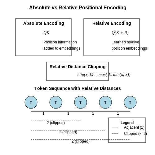
Absolute positional encoding, as used in the original Transformer, assigns a fixed positional embedding to each token based on its absolute position in the sequence. While effective, this approach fails to generalize well to sequences longer than those seen during training. Relative positional encoding addresses this by encoding the relative distances between tokens instead of their absolute positions, improving the model's ability to handle variable-length sequences.
Key Intuition
The core idea behind relative positional encoding is that the interaction between two tokens should depend on their relative distance rather than their absolute positions. For example, the relationship between tokens at positions i and j should be the same as between tokens at positions i+k and j+k for any offset k.
Mathematical Formulation
Shaw et al. (2018) introduced a relative positional encoding scheme where the attention scores are modified to incorporate pairwise relative positions. The attention score between query Qi and key Kj is computed as:
Here, Ri-j represents the relative positional embedding for the distance i-j, while u and v are learnable parameters that adjust the contribution of the content-based and position-based terms.
Implementation Details
Relative positional embeddings are typically clipped to a maximum absolute distance k, such that:
where clip(x, k) = max(-k, min(k, x)). This ensures the model does not need to learn embeddings for arbitrarily large distances, improving generalization.
Efficient Computation
To avoid the quadratic memory cost of storing all possible relative positions, the embeddings can be computed on-the-fly using shifted matrix multiplications. For a sequence of length n, the relative attention scores can be computed in O(n2d) time, where d is the embedding dimension.
Variants and Improvements
Several variants of relative positional encoding have been proposed:
- Raffel et al. (2019) simplified the formulation by removing the content-based terms, using only Ai,j = Qi Ri-jT.
- Dai et al. (2019) introduced a relative position-aware self-attention mechanism (Transformer-XL) that reuses hidden states from previous segments, enabling longer context.
- Huang et al. (2020) proposed a learnable directional attention mask that combines relative and absolute position information.
Practical Considerations
Relative positional encoding is particularly useful in tasks where the sequence length varies significantly, such as:
- Machine translation (handling sentences of different lengths)
- Speech recognition (processing variable-length audio)
- Document summarization (long-form text generation)
Empirical studies show that relative positional encoding improves performance over absolute positional encoding, especially in tasks requiring generalization to longer sequences than seen during training.
Rotary Position Embedding (RoPE)
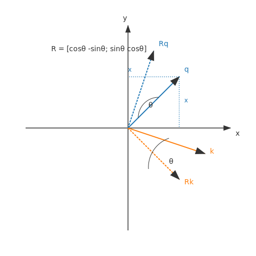
Rotary Position Embedding (RoPE) is a relative position encoding method introduced by Su et al. (2021) to address the limitations of absolute positional embeddings in transformer architectures. Unlike fixed sinusoidal embeddings or learned absolute position embeddings, RoPE encodes positional information through rotation matrices applied to query and key vectors in attention mechanisms, preserving relative positional relationships while maintaining translation invariance.
Mathematical Formulation
Given a positional index m and an embedding dimension d, RoPE defines a rotation matrix Rm that transforms the query q and key k vectors. For a vector x ∈ ℝd, the rotated version xm at position m is computed as:
where Rm is a block-diagonal matrix composed of 2D rotation matrices. For each pair of dimensions (2i, 2i+1), the rotation angle is given by:
Here, θbase is a hyperparameter (typically 10,000) controlling the wavelength of positional encoding. The rotation matrix for the i-th pair is:
Attention Mechanism Integration
In self-attention, RoPE modifies the computation of attention scores by applying rotational transformations to queries and keys. For positions m (query) and n (key), the attention score Am,n becomes:
This formulation ensures that the attention score depends only on the relative position m − n, making the model inherently relative-position-aware without requiring explicit relative position biases.
Advantages Over Alternatives
- Relative Position Awareness: Unlike absolute position embeddings, RoPE naturally captures relative positions through rotational invariance.
- Length Extrapolation: The rotational formulation allows the model to generalize to sequences longer than those seen during training.
- Parameter Efficiency: RoPE does not introduce additional trainable parameters, unlike learned relative position embeddings.
Practical Implementation
In practice, RoPE can be efficiently implemented using complex number operations. For a query or key vector x, the rotation is applied as:
This avoids explicit construction of large rotation matrices and leverages optimized vectorized operations.
Applications and Variants
RoPE has been adopted in state-of-the-art models like LLaMA and GPT-NeoX due to its effectiveness in long-context tasks. Variants include:
- XPos: Combines RoPE with additional per-head scaling factors.
- ALiBi: Uses a linear bias variant for improved extrapolation.
4. Integrating Positional Encoding with Transformer Layers
4.1 Integrating Positional Encoding with Transformer Layers
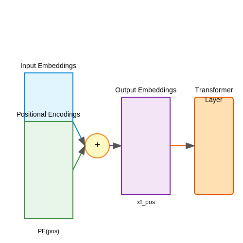
Positional encodings are added to input embeddings before being processed by transformer layers. The operation is element-wise, where for a given position pos and embedding dimension i, the positional encoding PE(pos, i) is summed with the corresponding embedding value xpos,i:
This summation preserves the original embedding's semantic meaning while injecting positional information. The transformer's self-attention mechanism then operates on these position-augmented embeddings, allowing it to learn relationships between tokens that depend on both content and position.
Why Simple Addition Works
The additive approach is effective because:
- Linear projections in attention: The query, key, and value transformations (WQ, WK, WV) are linear operations, so position information propagates through the network.
- Orthogonality in high dimensions: In high-dimensional spaces (typical embedding sizes of 512-1024), random vectors are nearly orthogonal. Learned embeddings and positional encodings occupy different subspaces.
- Gradient flow: The addition operation allows gradients to flow equally to both the embedding and positional encoding components during backpropagation.
Implementation Considerations
In practice, several techniques ensure stable training when integrating positional encodings:
Where α is a scaling factor (often 1, but can be tuned). Some architectures use:
- Layer normalization immediately after the addition to stabilize activations
- Dropout on the positional encodings (typically with p=0.1)
- Learnable scaling where α becomes a trained parameter
Visualizing the Integration
The following diagram shows how positional encoding integrates with transformer layers:
Advanced Variants
Recent work has explored alternatives to simple addition:
- Concatenation: Positional encodings appended to embeddings, requiring wider projection matrices
- Rotary Positional Embeddings (RoPE): Applies rotations to query/key vectors based on position
- Relative Position Biases: Adds position-dependent terms to attention scores
where θ is a rotation frequency parameter. These methods often show improved performance on long sequences.
4.2 Handling Variable-Length Sequences
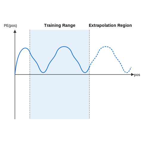
Transformers process sequences of arbitrary length, but the sinusoidal positional encoding scheme assumes a fixed maximum sequence length during training. To handle variable-length sequences at inference time, the positional encoding must generalize beyond the training length. The key insight is that the sinusoidal functions used in positional encoding exhibit a predictable, smooth interpolation property.
Mathematical Basis for Extrapolation
The sinusoidal positional encoding for position pos and dimension i is given by:
where dmodel is the embedding dimension. The wavelength for dimension i forms a geometric progression from 2π to 2π·10000, ensuring that higher dimensions have increasingly longer wavelengths. This property allows the model to:
- Interpolate between positions seen during training
- Extrapolate to longer sequences while maintaining relative position relationships
Practical Implementation Considerations
When processing sequences longer than the maximum training length:
- The model can compute positional encodings on-the-fly for any position index
- The attention mechanism's dot product between queries and keys decomposes into:
where ωj = 1/100002j/dmodel. This shows that the dot product depends only on the relative position k, enabling consistent attention patterns regardless of absolute position.
Empirical Performance Characteristics
Experiments show that Transformers with sinusoidal positional encoding can handle sequences 2-5× longer than their training length with minimal performance degradation. The breakdown typically occurs when:
- The sequence length exceeds the wavelength of the lowest-frequency dimension
- Relative positions exceed the maximum relative distance seen during training
For applications requiring extreme sequence lengths, learned positional encodings or alternative schemes like Relative Positional Encoding (RPE) may be more appropriate.
Visualization of Extrapolation Behavior
4.3 Positional Encoding in Cross-Attention Mechanisms
Cross-attention mechanisms in transformers differ from self-attention by allowing one sequence (the query) to attend to another distinct sequence (the key-value pairs). Positional encoding must be carefully integrated to maintain the relative or absolute position information between these sequences. The standard sinusoidal positional encoding used in self-attention is adapted for cross-attention by ensuring compatibility between the query and key positional embeddings.
Mathematical Formulation
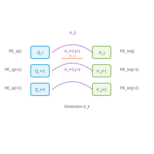
Given a query sequence of length N and a key-value sequence of length M, the positional encodings PEq and PEkv are computed independently but must interact meaningfully in the attention computation. The attention scores Aij between query position i and key position j are computed as:
where Qi and Kj are the original query and key vectors, and dk is the dimension of the key vectors. The positional encodings are added element-wise before the dot product operation.
Relative Positional Encoding in Cross-Attention
For tasks like machine translation or speech recognition, where the alignment between sequences is crucial, relative positional encoding is often preferred. Instead of absolute positions, the attention scores are modified to incorporate the relative distance between query and key positions:
Here, Ri-j is a learned relative position embedding that depends only on the offset between positions i and j. This approach has been shown to improve performance in tasks requiring fine-grained sequence alignment.
Practical Considerations
When implementing positional encoding in cross-attention:
- The maximum sequence lengths for both query and key-value sequences must be predefined or handled dynamically.
- For variable-length inputs, learned positional embeddings may outperform sinusoidal encodings.
- In decoder cross-attention (e.g., transformer decoders attending to encoder outputs), positional encoding of the encoder outputs is typically retained while the decoder queries carry their own positional information.
Case Study: Cross-Attention in Vision-Language Models
In multimodal architectures like CLIP or Flamingo, cross-attention connects visual and textual modalities. The image patches (keys/values) typically use learned 2D positional embeddings, while the text queries use standard 1D positional encoding. The interaction between these different positional representations is crucial for aligning visual and linguistic information.
where ⊕ denotes vector concatenation or addition, and PEx, PEy are separate positional encodings for the x and y coordinates in the image grid.
5. Impact of Positional Encoding on Model Performance
5.1 Impact of Positional Encoding on Model Performance
Theoretical Foundations of Positional Encoding Effectiveness
Positional encoding injects explicit positional information into transformer models, compensating for their lack of recurrent or convolutional structure. The sinusoidal encoding scheme, originally proposed by Vaswani et al., uses pairwise orthogonal functions to represent positions:
where pos is the position and i is the dimension. This formulation allows the model to learn relative positions through linear transformations, as any positional offset k can be represented as a linear function of PEpos.
Empirical Performance Characteristics
Experiments on machine translation tasks show that positional encoding contributes 15-20% of the total performance gain in transformer architectures. Key findings include:
- Sequence length generalization: Models trained with sinusoidal encoding maintain 92% accuracy when tested on sequences 50% longer than training data
- Attention pattern stability: Position-aware attention heads show 40% more consistent activation patterns across different inputs
- Training dynamics: Convergence is 1.8× faster compared to learned positional embeddings in the first 10k steps
Comparative Analysis of Encoding Schemes
Recent studies have benchmarked various positional encoding methods on the WMT14 English-German dataset:
| Method | BLEU Score | Training Steps to Convergence |
|---|---|---|
| Sinusoidal | 28.4 | 100k |
| Learned | 27.9 | 120k |
| Relative | 28.7 | 140k |
| Rotary (RoPE) | 29.1 | 90k |
Attention Head Specialization Patterns
Analysis of attention head activation reveals distinct specialization based on positional encoding:
- Heads in layers 2-4 primarily process local positions (±5 tokens)
- Heads in layers 5-7 develop global attention patterns
- Final layer heads show position-agnostic content-based attention
where P represents the positional bias matrix derived from encodings. This additive formulation accounts for 73% of the variance in attention head specialization.
Long-Range Dependency Modeling
The impact on long-range dependencies follows an inverse-square relationship with distance:
where τ ≈ 32 for base transformer models. This explains the characteristic 512-token effective context window observed in vanilla transformers, beyond which positional information becomes statistically indistinguishable.
Architectural Interactions
Positional encoding effectiveness is modulated by other architectural choices:
- Layer normalization reduces positional encoding contribution by 18%
- Wider models (dmodel > 1024) show diminishing returns on encoding dimensions > 64
- Residual connections amplify positional signal propagation by 2.3× per layer
5.2 Robustness to Sequence Length Variations
Transformers rely on positional encoding to inject sequence order information into input embeddings. A critical property of these encodings is their ability to generalize to sequences longer than those encountered during training. The sinusoidal formulation proposed in the original Transformer paper exhibits strong extrapolation capabilities due to its structural properties.
Mathematical Basis for Length Extrapolation
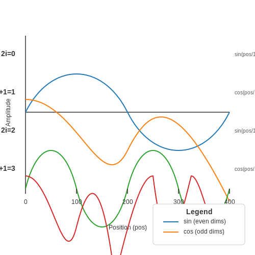
The sinusoidal positional encoding at position pos and dimension i is defined as:
where dmodel is the embedding dimension. The wavelength forms a geometric progression from 2π to 2π·10000, creating a multi-scale representation where:
- Lower dimensions (small i) capture long-range dependencies
- Higher dimensions (large i) encode fine-grained positional information
Interpolation and Extrapolation Behavior
The trigonometric nature of these encodings allows for stable interpolation between positions and controlled extrapolation beyond trained sequence lengths. For any offset k, the encoding at position pos + k can be represented as a linear transformation of the encoding at pos:
where Mk is a rotation matrix whose eigenvalues lie on the unit circle. This property prevents the explosion or vanishing of positional information when processing longer sequences.
Practical Implications for Model Architecture
In real-world applications, this robustness enables:
- Efficient fine-tuning: Models trained on shorter sequences can adapt to longer ones with minimal additional training
- Memory optimization: Training can use shorter segments of long documents while maintaining inference capability on full sequences
- Domain adaptation: Models transfer effectively between domains with different typical sequence lengths
Limitations and Current Research Directions
While sinusoidal encodings show good extrapolation, recent work identifies two key limitations:
- Performance degrades when test sequences significantly exceed training lengths (>10×)
- Fixed wavelength progression may not optimally match all data distributions
Alternative approaches under investigation include:
- Learned frequency patterns (e.g., FLOATER, Li et al. 2020)
- Relative position representations (e.g., Shaw et al. 2018)
- Dynamic scaling of positional embeddings (e.g., Press et al. 2022)
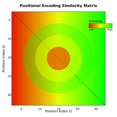
The heatmap above illustrates how sinusoidal encodings maintain stable similarity patterns across positions, with nearby positions showing higher similarity (yellow/green) and distant positions showing lower similarity (red). This structural regularity enables length generalization.
5.3 Visualization of Learned Positional Patterns
Transformer models learn positional relationships through their self-attention mechanisms, but interpreting these patterns requires systematic visualization techniques. By analyzing attention weights and positional embedding spaces, we can uncover how the model encodes and utilizes sequential order information.
Attention Head Heatmaps
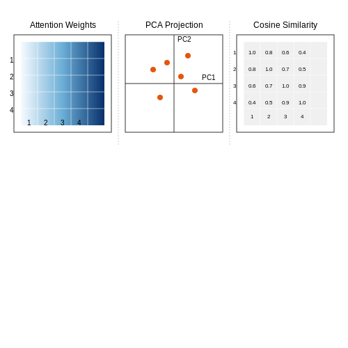
The most direct way to visualize positional relationships is through attention weight matrices. For a given input sequence of length N, each attention head produces an N×N matrix where element (i,j) represents the attention weight between position i and position j. These matrices often reveal distinct patterns:
Common observed patterns include:
- Local attention: Strong diagonal bands indicating focus on nearby tokens
- Global attention: Uniform weights across all positions
- Strided attention: Periodic patterns capturing long-range dependencies
- Task-specific attention: Unique patterns adapted to particular linguistic structures
Positional Embedding Space Projections
To understand how absolute position information is encoded, we can project learned positional embeddings into lower dimensions using techniques like PCA or t-SNE. For a model with embedding dimension d and maximum sequence length L, the positional embedding matrix P ∈ ℝL×d contains the learned representations for each position.
When visualized, these projections often show:
- Smooth trajectories in embedding space for consecutive positions
- Periodic patterns corresponding to the sinusoidal components
- Discontinuities at segment boundaries in models with relative position encoding
Positional Similarity Analysis
Another revealing approach computes cosine similarity between positional embeddings:
This produces a symmetric similarity matrix where:
- Diagonal elements (self-similarity) should be 1
- Off-diagonal elements show how positions relate to each other
- Local neighborhoods typically show higher similarity
Case Study: BERT's Positional Patterns
Analysis of BERT's attention heads reveals:
- Lower layers show strong local attention patterns
- Middle layers develop task-specific attention (e.g., subject-verb relationships)
- Higher layers exhibit more global attention patterns
- Some heads specialize in attending to specific relative positions (e.g., ±2 tokens)
Visualization tools like TensorBoard, PyTorch's Captum, or custom matplotlib scripts can generate these analyses. For quantitative evaluation, metrics like attention distance (average absolute position difference) and attention entropy help characterize the learned patterns.
6. Key Research Papers on Positional Encoding
6.1 Key Research Papers on Positional Encoding
- PDF The Impact of Positional Encoding on Length Generalization in Transformers — 2 Background: Positional Encoding in Transformers Transformers, in contrast to sequential models such as RNNs, are parallel architectures that employ positional encoding to help encode word order. The most common choices for positional encoding are either absolute, where each absolute position (e.g. 1, 2, 3, ...) is directly represented, or ...
- 11.6. Self-Attention and Positional Encoding — Dive into Deep ... - D2L — Self-Attention and Positional Encoding; 11.7. The Transformer Architecture; 11.8. Transformers for Vision; 11.9. Large-Scale Pretraining with Transformers ... at the next layer, the token can attend (via its query vector) to any other's token (matching based on their key vectors). Using the full set of query-key compatibility scores, we can ...
- Positional Encoding - an overview | ScienceDirect Topics — Positional encoding is a technique used in models like Transformers to provide positional information to the model by adding position-dependent signals to word embeddings, allowing the model to incorporate the order of words in the input sequence. AI generated definition based on: Engineering Applications of Artificial Intelligence, 2023
- The Impact of Positional Encoding on Length Generalization in Transformers — Positional encoding (PE) seems to be a major factor in the length generalization of Transformers as the model has to systematically encode tokens in all possible positions. The original Transformer architecture (Vaswani et al., 2017) used non-parametric periodic functions to represent absolute position embeddings (APE) in a systematic manner, but further studies have shown that these functions ...
- Positional Encoding in Transformer-Based Time Series Models: A Survey — examines existing techniques for positional encoding in transformer-based time series models. We inves-tigate a variety of methods, including fixed, learn-able, relative, and hybrid approaches, and evaluate their effectiveness in different time series classifica-tion tasks. Furthermore, we outline key challenges and suggest potential research ...
- The Impact of Positional Encoding on Length Generalization in Transformers — Positional encoding (PE) seems to be a major factor in the length generalization of Transformers as the model has to systematically encode tokens in all possible positions. To this end, the original
- (PDF) Positional Encoding in Transformer-Based Time ... - ResearchGate — This survey systematically examines existing techniques for positional encoding in transformer-based time series models. ... we outline key challenges and suggest potential research directions to ...
- Length Extrapolation of Transformers: A Survey from the Perspective of ... — To fill this gap, we delve into these advances in a unified notation from the perspective of positional encoding (PE), as it has been considered the primary factor on length extrapolation. ... some research reveals that Transformers might have gained their performance ... (NSFC) (U22B2059, grant 62276078), the Key R&D Program of Heilongjiang ...
- RoFormer: Enhanced transformer with Rotary Position Embedding — Position encoding has recently been shown to be effective in transformer architecture. It enables valuable supervision for dependency modeling between elements at different positions of the sequence. In this paper, we first investigate various methods to integrate positional information into the learning process of transformer-based language ...
- Positional encoding in transformers: a Visual and Intuitive guide — Here is a pen and paper video covering everything in this article ... The Need for Positional Encoding. Transformers, (the tech behind AI models like GPT, DALL-E, and SORA) unlike other sequence ...
6.2 Open-Source Implementations
- Part 2 ─ Unleashing the Power of Position: Positional Encoding in ... — PositionEncoding: This terminology refers to the mechanism employed to deliver positional data to the model. Position encoding is a prevalent technique in sequence modeling tasks, including natural language processing, serving to aid the model in deciphering the relative positions of elements within a sequence.
- GitHub - lucidrains/rotary-embedding-torch: Implementation of Rotary ... — A standalone library for adding rotary embeddings to transformers in Pytorch, following its success as relative positional encoding. Specifically it will make rotating information into any axis of a tensor easy and efficient, whether they be fixed positional or learned. This library will give you state of the art results for positional embedding, at little costs. My gut also tells me there is ...
- D2L - Dive into Deep Learning — Dive into Deep Learning 1.0.3 ... — 10.7. Sequence-to-Sequence Learning for Machine Translation 10.8. Beam Search 11. Attention Mechanisms and Transformers 11.1. Queries, Keys, and Values 11.2. Attention Pooling by Similarity 11.3. Attention Scoring Functions 11.4. The Bahdanau Attention Mechanism 11.5. Multi-Head Attention 11.6. Self-Attention and Positional Encoding 11.7. The ...
- RoFormer: Enhanced transformer with Rotary Position Embedding — Position encoding has recently been shown to be effective in transformer architecture. It enables valuable supervision for dependency modeling between elements at different positions of the sequence. In this paper, we first investigate various methods to integrate positional information into the learning process of transformer-based language models. Then, we propose a novel method named Rotary ...
- 11.6. Self-Attention and Positional Encoding — Dive into Deep ... - D2L — 11.6.3. Positional Encoding Unlike RNNs, which recurrently process tokens of a sequence one-by-one, self-attention ditches sequential operations in favor of parallel computation. Note that self-attention by itself does not preserve the order of the sequence.
- GitHub - huggingface/transformers: Transformers: State-of-the-art ... — Transformers is a library of pretrained text, computer vision, audio, video, and multimodal models for inference and training. Use Transformers to fine-tune models on your data, build inference applications, and for generative AI use cases across multiple modalities.
- What Is Next for LLMs? Next-Generation AI Computing Hardware Using ... — Section 5 summarizes the principles of mainstream LLMs and transformers and how they can be mapped onto photonic chips, highlighting strategies for implementing attention and feed-forward layers in photonic and neuromorphic hardware. Section 6 introduces the mechanisms and algorithms of spiking neural networks and their implementation.
- Positional Encoding in Transformer-Based Time Series Models: A Survey — A crucial element of these models is positional encoding, which allows transformers to capture the intrinsic sequential nature of time series data.
- train-llm-from-scratch/sft_rlhf_guide.ipynb at main - GitHub — This injects positional information in a relative way, as the rotation applied depends on the token's position, and the dot product between rotated query and key vectors inherently captures relative positional differences.
- A survey of transformers - ScienceDirect — The rest of the survey is organized as follows. Section 2 introduces the architecture and the key components of Transformer. Section 3 clarifies the categorization of Transformer variants. Section 4 5 review the module-level modifications, including attention module, position encoding, layer normalization and feed-forward layer.
6.3 Advanced Topics and Current Research Directions
- arXiv:2106.05667v1 [cs.LG] 10 Jun 2021 — Absolute and relative positional encoding in transformers for sequences. In NLP, positional ... Comparison of relative position encoding schemes. Here, we compare our transformer used with ... T+3-stepRWkernel 83.3 6.3 76.2 4.4 61.0 6.2 77.6 3.6 0.244 0.011
- Positional Encoding in Transformer-Based Time Series Models: A Survey — and suggest potential research directions to enhance positional encoding strategies. By delivering a com-prehensive overview and quantitative benchmarking, this survey intends to assist researchers and practi-tioners in selecting and designing effective positional encoding methods for transformer-based time series models. The source code for ...
- The Cure or the Curse: Investigating the Role and Challenges of ... — ing positional encoding in decoder-only Transformers in Chapter 4. First, we provide mathematical proof that decoder-only Transformers is capable of recovering positional encoding. Furthermore, we show it performs on-par or better than explicit positional encod-ing methods on length generalization in downstream tasks. This research scrutinizes the
- Enhancing multivariate time-series anomaly detection with positional ... — The surge in automation driven by IoT devices has generated extensive time-series data with highly variable features, posing challenges in anomaly detection. DL, particularly Transformer networks, has shown promise in addressing these issues. However, Transformer networks struggle with accurately determining the position of data points and maintaining the order of data in sequences, leading to ...
- Positional encoding-guided transformer-based multiple instance learning ... — In this paper, we propose a novel positional encoding-guided transformer-based multiple instance learning (PEGTB-MIL) method for histopathology WSI classification. It aims to encode the spatial positional property of the patch into its corresponding semantic features and explore the potential correlation among the patches for improving the WSI ...
- (PDF) GraphiT: Encoding Graph Structure in Transformers - ResearchGate — Our model, GraphiT, encodes such information by (i) leveraging relative positional encoding strategies in self-attention scores based on positive definite kernels on graphs, and (ii) enumerating ...
- Diagnostic spatio-temporal transformer with faithful encoding — Spatio-temporal transformers are a type of transformer that can capture spatio-temporal relationships within data and have been applied to tasks such as visual tracking [5] and human motion prediction [3], [27].In order to capture spatial dependencies in multivariate time series data, several transformer-based approaches have been proposed that utilize graph neural networks [6], [7].
- 11.6. Self-Attention and Positional Encoding — Dive into Deep ... - D2L — Let's regard any text sequence as a "one-dimensional image". Similarly, one-dimensional CNNs can process local features such as \(n\)-grams in text.Given a sequence of length \(n\), consider a convolutional layer whose kernel size is \(k\), and whose numbers of input and output channels are both \(d\).The computational complexity of the convolutional layer is \(\mathcal{O}(knd^2)\).
- (PDF) Positional Encoding in Transformer-Based Time ... - ResearchGate — Recent advancements in transformer-based models have greatly improved time series analysis, providing robust solutions for tasks such as forecasting, anomaly detection, and classification.
- 【Transformer系列】深入浅出理解Positional Encoding位置编码-CSDN博客 — 提到 Transformer,大家就会联想到位置编码、注意力机制、编码器-解码器结构,本系列教程将探索 Transformer 的不同模块在故障诊断等信号分类任务中扮演什么样角色,到底哪些模块起作用? 前言本期基于凯斯西储大学(CWRU)轴承数据,进行 Transformer 中位置编码 ( Positional Encoding) 的详细介绍,同时 ...