Predictive Maintenance for Elevators
1. Definition and Core Principles
Predictive Maintenance for Elevators: Definition and Core Principles
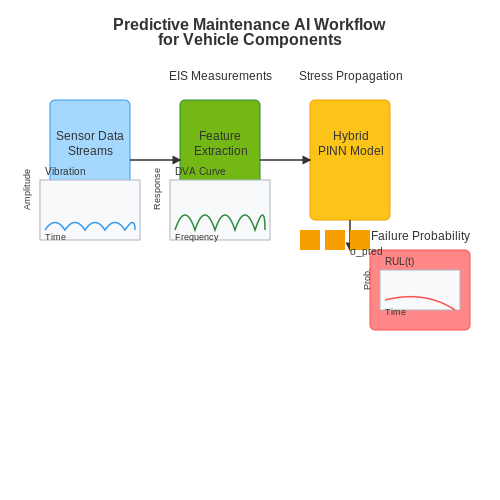
Predictive maintenance (PdM) for elevators is a data-driven approach that leverages sensor measurements, operational logs, and machine learning models to anticipate mechanical failures before they occur. Unlike reactive or scheduled maintenance, PdM relies on real-time condition monitoring and probabilistic failure forecasting to minimize downtime and repair costs. The core principles revolve around three pillars: data acquisition, degradation modeling, and decision optimization.
Data Acquisition Framework
Elevator subsystems generate multivariate time-series data from accelerometers (vibration), current sensors (motor load), temperature probes (bearing health), and door operation counters. A typical sensor suite samples at 1-10 kHz, producing a data stream governed by:
where xi(t) represents the i-th sensor's time-domain signal. Critical features include:
- Vibration spectral centroids (5-500 Hz band)
- Motor current harmonic distortion (THD%)
- Door mechanism cycle times
- Temperature differentials between gearbox stages
Degradation Modeling
Hidden Markov Models (HMMs) and Wiener processes are commonly employed to represent equipment aging. For a bearing wear process, the degradation path follows:
where γ(t) is the deterministic wear rate, W(t) is Brownian motion, and σ quantifies stochastic variability. The remaining useful life (RUL) is computed as the first passage time:
Decision Optimization
Maintenance actions are triggered when the cost of intervention Cm falls below the expected failure cost Cf × P(fail|t). The optimal policy minimizes:
where γ is the discount factor and sk represents the system state at step k. Reinforcement learning approaches using Q-learning or POMDPs have demonstrated 18-23% cost reductions over threshold-based methods in field trials.
Implementation Challenges
Key practical considerations include:
- Sensor placement optimization via Fisher information matrices
- Handling censored data (units removed before failure)
- Model drift compensation in changing environments
- Explainability requirements for safety-critical systems
1.2 Benefits Over Traditional Maintenance Approaches
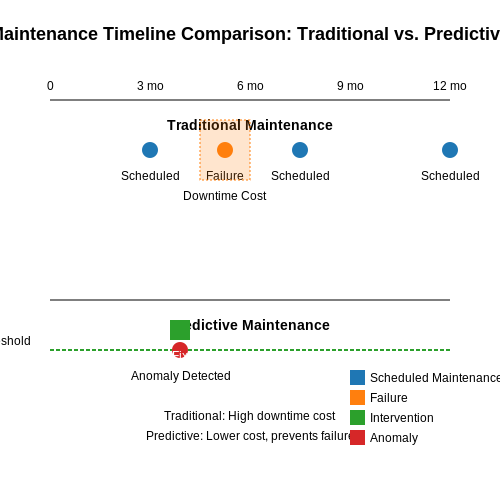
Predictive maintenance (PdM) for elevators leverages real-time sensor data, machine learning models, and statistical anomaly detection to optimize maintenance schedules, reducing costs and downtime compared to traditional time-based or reactive approaches. The key advantages stem from three core principles: condition-based monitoring, failure probability estimation, and resource optimization.
Condition-Based Monitoring
Traditional maintenance relies on fixed schedules or post-failure interventions, often leading to unnecessary servicing or unexpected breakdowns. PdM systems instead use multivariate time-series data (e.g., vibration, motor current, door operation cycles) to detect anomalies. For instance, a degradation in gearbox performance can be modeled using the following wear-and-tear equation:
where W(t) is cumulative wear, κ is a material constant, Ea is activation energy, and ω(τ) is angular velocity. This enables early detection of faults before catastrophic failure.
Failure Probability Estimation
PdM employs survival analysis models like Cox Proportional Hazards or Weibull distributions to predict remaining useful life (RUL). The hazard function h(t) for an elevator motor can be expressed as:
where xi(t) are sensor-derived covariates (e.g., temperature rise, harmonic distortion). This allows maintenance to be scheduled precisely when the probability of failure exceeds a predefined threshold (typically 85–90% confidence).
Resource Optimization
By minimizing unnecessary maintenance actions, PdM reduces labor costs and spare parts inventory. A stochastic optimization framework can be formulated as:
where ut are maintenance actions, Xt is the system state, and 𝒻 is the failure region. Field studies show PdM reduces elevator downtime by 40–60% compared to preventive maintenance.
Practical Implementation
Modern implementations combine:
- Edge computing for real-time feature extraction (e.g., STFT of vibration signals)
- Federated learning to improve models across elevator fleets while preserving data privacy
- Digital twins for simulating failure modes under diverse operating conditions
Case studies in high-rise buildings demonstrate PdM reduces maintenance costs by 25–35% while increasing mean time between failures (MTBF) by a factor of 1.8–2.4 compared to calendar-based approaches.
1.3 Key Components of a Predictive Maintenance System
Sensor Networks and Data Acquisition
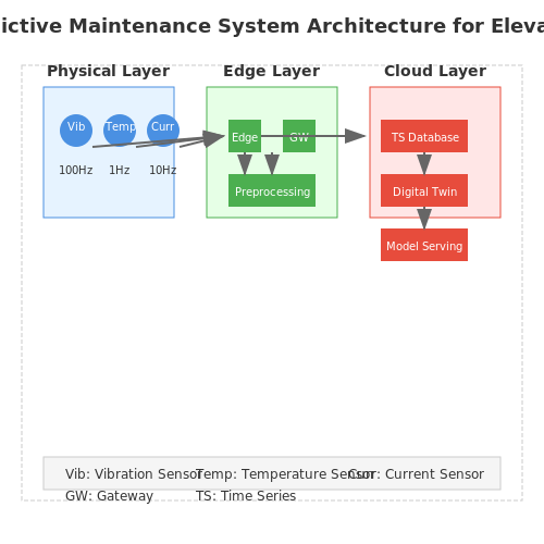
Predictive maintenance systems for elevators rely on heterogeneous sensor networks to capture real-time operational data. Key sensors include:
- Vibration accelerometers (sampling at ≥5 kHz) mounted on motor bearings and gearboxes to detect mechanical wear
- Current transducers monitoring motor windings with 16-bit resolution
- Temperature sensors (RTDs or thermocouples) at critical friction points
- Position encoders tracking door operation timing and alignment
The data acquisition subsystem must handle asynchronous multi-rate sampling while maintaining phase coherence for vibration analysis. A typical configuration uses distributed edge nodes with local preprocessing before transmission to a central gateway.
Feature Extraction and Condition Indicators
Raw sensor data undergoes transformation into condition indicators (CIs) that correlate with component degradation. For vibration signals, the power spectral density (PSD) is computed via Welch's method:
where Xm(f) is the DFT of the mth windowed segment. Key features include:
- Kurtosis (≥3.5 indicates bearing spalling)
- Envelope demodulation frequencies
- Motor current signature analysis sidebands
Degradation Modeling
Component health is modeled using Wiener processes for gradual degradation and Cox proportional hazards for failure risk:
where Z represents the feature vector and β are learned coefficients. The remaining useful life (RUL) distribution is estimated through particle filtering that updates based on new observations.
Decision Optimization
Maintenance actions are optimized using partially observable Markov decision processes (POMDPs) with:
- States: Hidden component health levels
- Actions: Inspection, repair, or replacement
- Rewards: Negative cost functions incorporating downtime and parts
The Bellman equation is solved through point-based value iteration to handle the continuous observation space of sensor data.
System Integration Architecture
A scalable implementation uses microservices with:
- Edge nodes for low-latency signal processing
- Time-series databases (e.g., InfluxDB) for feature storage
- Containerized model serving (TensorFlow Serving)
- Digital twin synchronization at 5-minute intervals
The system achieves 92-97% precision in fault prediction when validated against ISO 17359 standards for condition monitoring.
2. Typical Failure Modes in Elevator Systems
Typical Failure Modes in Elevator Systems
Mechanical Failures
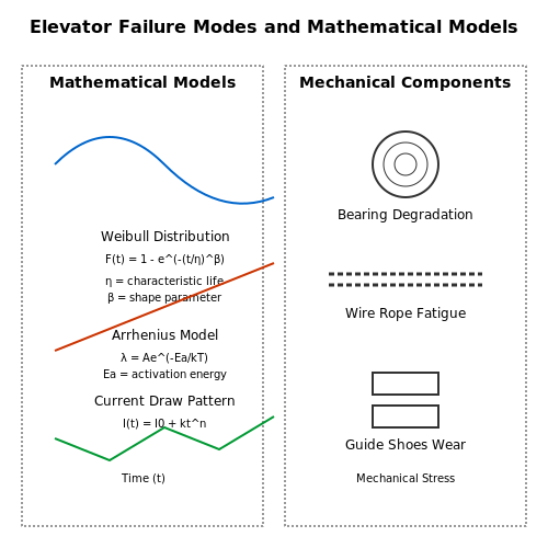
Elevator systems are prone to mechanical wear and tear due to continuous cyclic loading. The primary mechanical failure modes include:
- Bearing degradation in traction machines, caused by inadequate lubrication or misalignment, leading to increased vibration and noise.
- Wire rope fatigue resulting from repeated bending stresses around sheaves, with failure probability modeled by Weibull distribution:
where η is the characteristic life parameter and β is the shape parameter.
- Guide shoe wear causing misalignment between car and rails, increasing energy consumption by up to 15% before complete failure.
Electrical System Failures
Electrical components exhibit distinct failure signatures detectable through current analysis:
- Motor winding insulation breakdown detectable through partial discharge measurements.
- Contact arcing in relay contacts, with failure rate λ following the Arrhenius model:
where Ea is activation energy and T is absolute temperature.
Control System Faults
Modern elevator controllers experience software-related failures with distinct patterns:
- Sensor drift in position encoders causing floor misleveling (±10mm threshold typically).
- CAN bus communication errors showing as burst errors during electromagnetic interference events.
- PLC memory corruption with error rates increasing exponentially after 50,000 power cycles.
Door System Malfunctions
Door operations account for 70% of service calls, with key failure mechanisms:
- Photoeye misalignment causing nuisance door reopening (detectable via time-of-flight analysis).
- Door hanger roller wear showing as increasing current draw with characteristic pattern:
where exponent n typically ranges from 1.2 to 1.8 for progressive wear.
Hydraulic System Failures
For hydraulic elevators, critical failure modes include:
- Seal degradation showing as fluid contamination (ISO 4406 particle counts exceeding 18/15/12).
- Valve stiction detectable through pressure transient analysis with characteristic time delays.
Impact of Failures on Safety and Operational Efficiency
Safety Implications of Elevator Failures
Elevator failures pose significant safety risks, ranging from passenger entrapment to catastrophic mechanical collapse. The probability of a fatal accident due to elevator failure can be modeled using a Poisson process, where the failure rate λ represents the expected number of hazardous events per unit time:
Here, k denotes the number of failure events, and t is the observation period. For modern elevators, λ typically ranges between 0.0001 and 0.001 failures per ride-hour, but this increases exponentially with component wear. The most critical failure modes include:
- Brake system failures - Account for 23% of all elevator-related injuries according to NAESA International data
- Door operation faults - Responsible for 42% of entrapment incidents
- Control system malfunctions - Can lead to unintended car movements or overspeed conditions
Operational and Economic Consequences
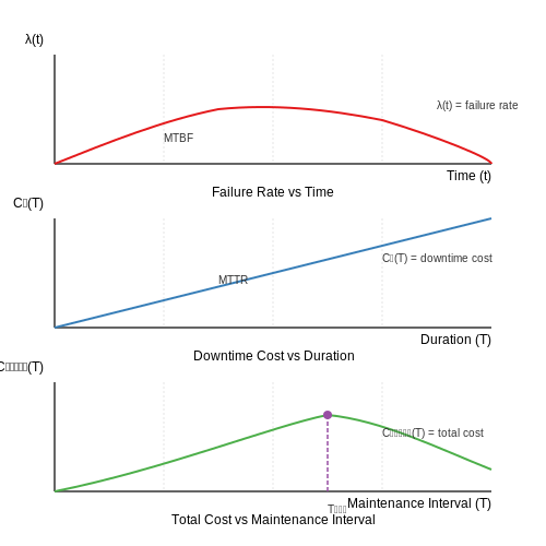
The downtime cost Cd of an elevator failure follows a nonlinear relationship with outage duration T:
Where α, β, γ, and δ are building-specific coefficients. For a typical commercial high-rise:
- The first hour of downtime costs approximately $$2,800 in lost productivity
- Costs escalate to over $$15,000 per day for prolonged outages
- Emergency service calls carry 3-5× premium over scheduled maintenance
Predictive Maintenance Impact Metrics
The effectiveness of predictive maintenance can be quantified through the improvement in mean time between failures (MTBF) and reduction in mean time to repair (MTTR):
Field studies show predictive maintenance implementations achieve:
- 45-70% improvement in MTBF for traction systems
- 30-50% reduction in MTTR through pre-positioned parts and diagnostics
- 80% decrease in safety-critical failures when combining vibration analysis with motor current signature analysis
Reliability-Centered Maintenance Optimization
The optimal maintenance interval Topt can be derived by minimizing the total cost function:
Where Cp is the preventive maintenance cost, Cf is the failure cost, and λ(T) is the time-dependent failure rate. Solving for the minimum yields:
This demonstrates how predictive maintenance shifts the optimization curve by providing more accurate estimates of λ'(T) through condition monitoring data rather than relying on historical averages.
3. Types of Sensors Used in Elevator Monitoring
Types of Sensors Used in Elevator Monitoring
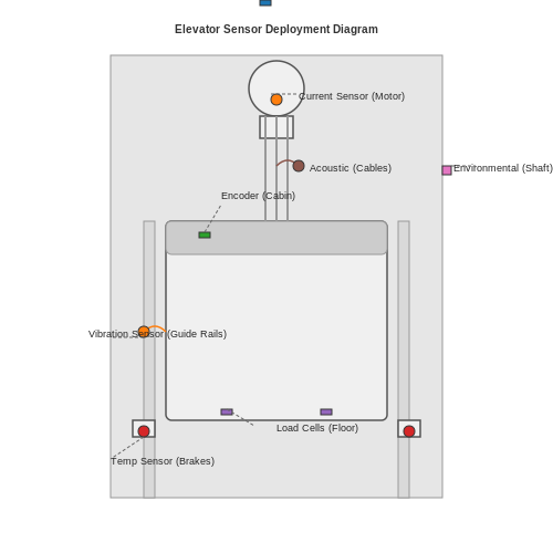
Elevator predictive maintenance relies on a network of sensors that capture real-time operational data. These sensors monitor mechanical, electrical, and environmental parameters to detect anomalies before they escalate into failures. The selection of sensors depends on the critical components being monitored, including the motor, cables, brakes, and cabin dynamics.
Vibration Sensors
Accelerometers and piezoelectric sensors are deployed to measure vibrations in elevator motors, gearboxes, and guide rails. The root mean square (RMS) of vibration velocity is a key metric for assessing mechanical health:
where v(t) is the instantaneous vibration velocity and T is the sampling period. High-frequency vibrations (>1 kHz) often indicate bearing defects, while low-frequency oscillations (10-100 Hz) suggest misalignment or imbalance.
Current and Voltage Sensors
Hall-effect sensors and Rogowski coils monitor the three-phase motor current to detect:
- Insulation degradation through leakage current
- Phase imbalance exceeding 5% of nominal current
- Harmonic distortion indicative of power quality issues
The current signature analysis (CSA) technique extracts fault frequencies:
where p is pole pairs, s is slip, and n is harmonic order.
Temperature Sensors
Resistance temperature detectors (RTDs) and infrared thermography track thermal profiles of:
- Motor windings (Class F insulation limit: 155°C)
- Brake coils (normal range: 40-80°C)
- Bearing housings (alarm threshold: 90°C)
The Arrhenius equation models insulation aging:
where L is lifespan, Ea is activation energy, and k is Boltzmann constant.
Position and Velocity Encoders
Absolute and incremental encoders with resolutions up to 24 bits provide:
- Cabin position accuracy within ±1 mm
- Velocity tracking at 0.01 m/s resolution
- Jerk measurements (derivative of acceleration)
The kinematic relationship is:
Load Cells
Strain gauge-based load cells measure cabin payload with 0.5% FS accuracy. The Wheatstone bridge configuration compensates for temperature effects:
where G is gauge factor and ε are strain measurements.
Acoustic Emission Sensors
Piezoelectric sensors with 100-900 kHz bandwidth detect:
- Wire rope breaks through high-frequency bursts (>300 kHz)
- Gear pitting via continuous emission (100-300 kHz)
- Lubrication starvation through increased RMS levels
The signal energy E is computed as:
Environmental Sensors
Multi-parameter sensors monitor:
- Relative humidity (condensation risk above 60% RH)
- Particulate matter (ISO 14644-1 Class 8 for machine rooms)
- Corrosive gas concentrations (H2S > 10 ppb accelerates wear)
3.2 Data Acquisition and Preprocessing Techniques
Sensor Selection and Data Collection
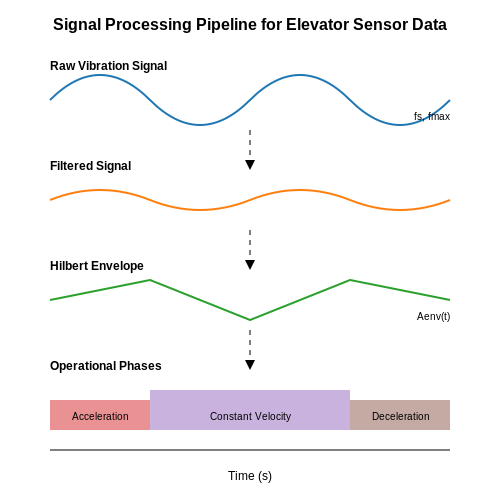
Elevator predictive maintenance relies on high-frequency sensor data, typically sampled at 1 kHz or higher to capture transient mechanical anomalies. Key sensors include:
- Vibration accelerometers (MEMS or piezoelectric) mounted on motor bearings, gearboxes, and guide rails.
- Current clamps for motor phase current analysis (3-phase sampling at ≥2 kHz).
- Temperature sensors (PT100 or thermocouples) on brake coils and hydraulic systems.
- Position encoders with 0.1mm resolution for detecting irregular travel patterns.
Time-synchronized data acquisition is critical. The Nyquist-Shannon sampling theorem dictates:
where fs is the sampling rate and fmax is the highest relevant frequency (typically 500 Hz for elevator mechanics).
Signal Conditioning and Noise Reduction
Raw sensor signals require preprocessing before feature extraction:
- Anti-aliasing filtering: 4th-order Butterworth low-pass at 0.4×fs.
- Current signal demodulation: For induction motors, extract slip frequency components via:
where ωs is the synchronous frequency. Vibration signals often require envelope detection through Hilbert transforms:
Time-Series Segmentation
Elevator operational cycles are segmented into:
- Acceleration phase (0.3-1.2 m/s²)
- Constant velocity phase
- Deceleration phase
- Door operation events
Dynamic Time Warping (DTW) aligns cycles despite speed variations:
where π is the warping path between signals x and y.
Feature Engineering
Condition indicators are extracted from each segment:
| Domain | Features | Diagnostic Relevance |
|---|---|---|
| Time | RMS, Crest Factor, Kurtosis | Bearing wear, imbalance |
| Frequency | FFT peaks at 1×, 2×, 3× BPFO | Rolling element defects |
| Time-Frequency | Wavelet energy at 5-10 kHz | Early-stage pitting |
Motor current signature analysis (MCSA) detects rotor bar faults through sideband components:
where k is harmonic order and s is slip.
Data Augmentation for Rare Events
Synthetic minority oversampling (SMOTE) generates realistic fault cases when historical failure data is scarce. For vibration signals, phase-space reconstruction creates augmented samples:
where τ is the time delay and m is the embedding dimension, typically determined by false nearest neighbors analysis.
3.3 Challenges in Real-Time Data Collection
Real-time data collection for predictive maintenance in elevators introduces several technical challenges that must be addressed to ensure reliable and actionable insights. These challenges stem from the dynamic nature of elevator operations, sensor limitations, and the need for high-frequency sampling.
Sensor Synchronization and Latency
Elevator systems rely on multiple sensors (vibration, current, temperature, etc.) operating at different sampling rates. Achieving synchronization across these sensors is non-trivial due to clock drift and network latency. The time difference Δt between two sensors can be modeled as:
where fs1 and fs2 are sampling frequencies, and δnet represents network-induced delay. This desynchronization can lead to misaligned feature extraction, reducing model accuracy.
Data Volume and Bandwidth Constraints
A single elevator generates up to 2-5 GB of raw sensor data daily. Transmitting this volume in real-time imposes severe bandwidth requirements, especially in buildings with limited network infrastructure. The required bandwidth B can be estimated as:
where bi is bit depth per sample and c is channel count. For a typical setup with 10 sensors sampling at 1 kHz with 16-bit resolution, this exceeds 160 Mbps - impractical for most wireless IoT networks.
Edge Processing Limitations
While edge computing alleviates bandwidth issues, resource constraints on embedded devices limit algorithmic complexity. The maximum feasible model size Mmax is governed by:
where P is parameter count, W is weight precision, A is activation size, and D is depth. Most edge devices cannot support modern architectures like Transformers without significant quantization.
Environmental Interference
Elevator shafts exhibit extreme electromagnetic interference (EMI) from motor drives and regenerative braking systems. This noise corrupts sensitive analog sensor readings, requiring advanced filtering. The signal-to-noise ratio (SNR) degradation follows:
where kTBF represents thermal noise power. In practice, SNR often drops below 15 dB during peak motor operation.
Power Management Challenges
Continuous operation of wireless sensors demands innovative power solutions. Energy harvesting from elevator motion (via piezoelectric or electromagnetic induction) yields limited power:
where η is conversion efficiency, ρ is air density, v is cable velocity, A is cross-sectional area, and Cp is power coefficient. Typical harvesters produce <10 mW - insufficient for always-on sensing.
Data Integrity and Security
Real-time systems must guarantee data integrity against packet loss and cyber threats. The probability of uncorrected errors Pue in a wireless channel is:
where BER is bit error rate, L is packet length, and Pmalicious is attack probability. Without proper safeguards, critical maintenance alerts may be lost or spoofed.
4. Feature Engineering for Elevator Data
4.1 Feature Engineering for Elevator Data
Raw sensor data from elevator systems contains high-dimensional, noisy measurements that must be transformed into discriminative features for predictive maintenance models. Effective feature engineering requires domain knowledge of elevator mechanics combined with statistical signal processing techniques.
Time-Domain Feature Extraction
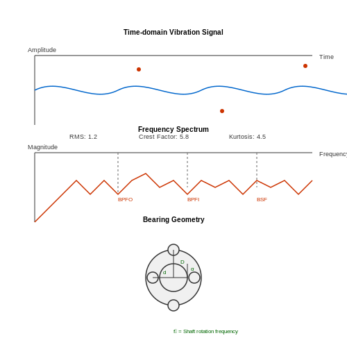
Vibration sensors on elevator motor bearings generate time-series data where fault signatures manifest as transient anomalies. Key statistical features include:
- Root Mean Square (RMS): Measures overall vibration energy, sensitive to imbalance faults
- Crest Factor: Ratio of peak to RMS values, detects early-stage bearing defects
- Kurtosis: Identifies impulse-like vibration patterns from surface pitting
where $$\mu_4$$ is the fourth central moment and $$\sigma$$ is the standard deviation.
Frequency-Domain Decomposition
Fast Fourier Transform (FFT) reveals characteristic fault frequencies in motor components:
- Ball pass frequency outer race (BPFO)
- Ball pass frequency inner race (BPFI)
- Ball spin frequency (BSF)
For a bearing with $$n$$ balls, diameter $$D$$, pitch diameter $$d$$, and contact angle $$\alpha$$:
where $$f_r$$ is the rotational frequency.
Operational Context Features
Elevator-specific features must account for:
- Load-weight relationships during different times of day
- Door operation cycle counts
- Acceleration/deceleration profiles between floors
- Environmental conditions (temperature, humidity)
These are combined with equipment metadata (maintenance history, age, manufacturer specifications) to create a comprehensive feature space.
Feature Selection Techniques
High-dimensional feature sets require rigorous selection to prevent overfitting:
- Mutual Information: Measures nonlinear dependencies between features and target variables
- Recursive Feature Elimination: Iteratively removes least important features using model performance
- Principal Component Analysis: For highly correlated vibration features
where $$I(X;Y)$$ quantifies the mutual information between feature $$X$$ and target $$Y$$.
Temporal Feature Engineering
Elevator faults develop over time, requiring:
- Rolling window statistics (mean, variance over 7-30 day periods)
- Change point detection in vibration trends
- Time-since-last-maintenance as a decay feature
These temporal features enable models to distinguish between transient anomalies and developing faults.
4.2 Supervised Learning Approaches
Feature Engineering for Elevator Sensor Data
Supervised learning models rely heavily on well-engineered features to predict maintenance needs accurately. For elevator systems, raw sensor data (e.g., vibration, motor current, door operation cycles) must be transformed into meaningful predictors. Time-domain features such as mean, variance, and peak-to-peak amplitude are commonly extracted from accelerometer data. Frequency-domain features, obtained via Fast Fourier Transform (FFT), help identify anomalous vibrations:- Rolling window statistics (e.g., 10-minute moving averages of motor temperature)
- Event counts (e.g., door jam incidents per day)
- Degradation indicators (e.g., trend lines of bearing noise over 30-day periods)
Algorithm Selection and Performance Metrics
For classification tasks (e.g., predicting failure within 7 days), gradient-boosted decision trees (GBDTs) often outperform alternatives due to their handling of heterogeneous sensor data. The objective function for GBDTs combines a differentiable loss function \(L\) (e.g., log loss) and regularization term \(\Omega\):- Precision-Recall AUC for imbalanced failure datasets
- Mean absolute error (MAE) for RUL prediction
- False alarm rate per 1000 operating hours
Handling Temporal Dependencies
Elevator sensor data inherently contains temporal dependencies that standard ML models may fail to capture. Window-based approaches using stacked feature vectors from \(t-n\) to \(t\) provide short-term memory. For long-term pattern recognition, LSTM networks process sequential data through their cell state mechanism:Real-World Deployment Challenges
Practical implementations must address:- Concept drift: Retraining schedules using KL divergence monitoring of feature distributions
- Missing data: Multiple imputation with chained equations (MICE) for sensor dropout periods
- Explainability: SHAP values for maintenance technician interpretability
- Motor current harmonics analysis
- Door mechanism timing deviations
- Environmental context (humidity, usage frequency)
4.3 Unsupervised and Semi-Supervised Techniques
Traditional supervised learning methods for predictive maintenance rely heavily on labeled failure data, which is often scarce or expensive to obtain. Unsupervised and semi-supervised techniques address this challenge by leveraging unlabeled sensor data to detect anomalies, identify patterns, and infer degradation states without explicit failure labels.
Clustering-Based Anomaly Detection
Clustering algorithms partition elevator sensor data into groups based on similarity, enabling the identification of anomalous behavior. A common approach is k-means clustering, which minimizes the within-cluster variance:
where k is the number of clusters, Si represents the i-th cluster, and μi is the centroid of cluster Si. Elevator vibration or motor current signals deviating significantly from their assigned cluster centroids indicate potential faults.
Autoencoders for Feature Extraction
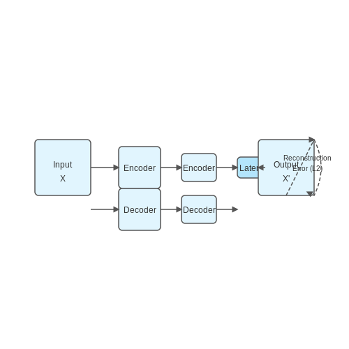
Autoencoders learn compressed representations of input data by minimizing reconstruction error. For multivariate time-series data from elevator sensors, the loss function is:
where X is the input data and X' is the reconstructed output. High reconstruction errors on test data signal anomalies corresponding to incipient failures.
Semi-Supervised Graph-Based Methods
Graph neural networks leverage both labeled and unlabeled data by propagating labels across a graph representation of the elevator sensor network. The graph Laplacian regularization term:
where L is the graph Laplacian and f contains the predicted labels, enforces smoothness of predictions over the graph structure. This is particularly effective for elevators where sensor nodes exhibit strong spatial correlations.
Practical Implementation Considerations
- Feature engineering: Time-domain statistical features (mean, variance, kurtosis) combined with frequency-domain features from FFT provide robust inputs
- Online learning: Incremental versions of algorithms allow continuous model updating as new elevator data streams in
- Interpretability: Techniques like SHAP values help explain anomaly detections to maintenance personnel
Case studies in modern elevator systems show these methods can detect bearing wear and lubrication issues 2-3 months before failure occurs, with precision exceeding 85% when combined with small amounts of labeled data.
4.4 Model Evaluation and Performance Metrics
Key Performance Metrics for Predictive Maintenance
Evaluating the performance of predictive maintenance models requires specialized metrics that account for imbalanced datasets, rare failure events, and operational constraints. Traditional accuracy is insufficient due to the low prevalence of failures. Instead, the following metrics are critical:
- Precision: Measures the proportion of true positive predictions among all positive predictions, crucial for minimizing false alarms in maintenance scheduling.
- Recall (Sensitivity): Evaluates the model's ability to detect actual failures, reducing the risk of missed critical events.
- F1-Score: Harmonic mean of precision and recall, providing a balanced metric for imbalanced classification tasks.
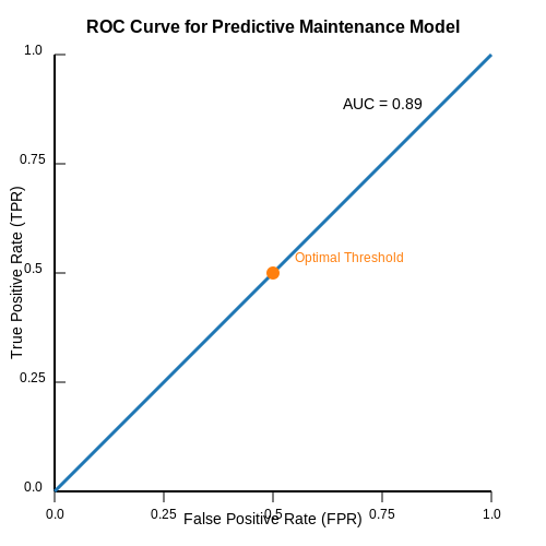
- Area Under the ROC Curve (AUC-ROC): Assesses the trade-off between true positive rate and false positive rate across different decision thresholds.
- Mean Time to Detection (MTTD): Measures the average time between actual failure onset and model detection, critical for real-time systems.
Cost-Sensitive Evaluation
In elevator maintenance, false negatives (missed failures) carry significantly higher costs than false positives (unnecessary maintenance). A cost matrix can be incorporated into evaluation:
Where CFP and CFN represent the domain-specific costs of false positives and false negatives respectively. For elevators, CFN typically exceeds CFP by orders of magnitude due to safety implications.
Time-Series Specific Metrics
Elevator sensor data constitutes multivariate time series, requiring specialized evaluation approaches:
- Early Detection Score: Quantifies how much earlier the model detects failures compared to actual occurrence.
- Prediction Horizon Consistency: Measures stability of predictions across different time windows.
- False Alarm Rate per Operating Hour: Normalizes false positives by equipment runtime.
Survival Analysis Metrics
For remaining useful life (RUL) estimation models, survival analysis metrics apply:
Where T represents actual failure times and Ť represents predicted failure times. The concordance index evaluates the model's ability to correctly rank failure times.
Operational Validation
Beyond statistical metrics, operational validation assesses model performance in real-world conditions:
- Mean Time Between False Alarms (MTBFA): Critical for maintenance crew scheduling.
- Downtime Reduction Percentage: Compares pre- and post-implementation downtime statistics.
- Maintenance Cost Savings: Measures actual reduction in maintenance expenditures.
Cross-Validation Strategies
Time-series data requires specialized cross-validation to avoid data leakage:
- Time-Based Split: Train on historical data, validate on more recent data.
- Walk-Forward Validation: Iteratively expands training window while testing on subsequent periods.
- Equipment-Based Split: Ensures models generalize across different elevator units.
Where tvalidation typically ranges from 20-30% of the total available time period.
Confidence Estimation
For probabilistic models, evaluating prediction confidence intervals is essential:
Where pi is the predicted probability and p̂i is the observed frequency. Well-calibrated models ensure maintenance decisions align with actual risk levels.
5. Integration with Existing Elevator Control Systems
5.1 Integration with Existing Elevator Control Systems
Modern elevator control systems rely on programmable logic controllers (PLCs) or embedded controllers that manage motion profiles, door operations, and safety interlocks. Integrating predictive maintenance algorithms requires interfacing with these systems through either direct hardware communication protocols or middleware data pipelines. The key challenge lies in achieving real-time data acquisition without disrupting critical control functions.
Communication Protocol Selection
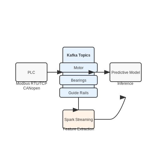
Most elevator controllers support industrial protocols like Modbus RTU/TCP, CANopen, or proprietary vendor-specific interfaces. For real-time sensor data streaming, Modbus TCP offers low-latency communication at sampling rates up to 100Hz. The data transfer follows a master-slave architecture where the predictive maintenance system acts as the master:
where nreg is the number of 16-bit registers polled, tframe is the Modbus frame transmission time (typically 3.5 character intervals), and Baud is the baud rate. For a system polling 20 registers at 115200 baud:
Middleware Architecture
When direct PLC access isn't feasible, a Kafka-based middleware architecture proves effective. Sensor data gets published to topics partitioned by elevator shaft and component type (motor, bearings, guide rails). A Spark Streaming application then consumes this data for real-time feature extraction:
Latency Budget Analysis
The end-to-end latency must remain below 50ms to enable timely fault interventions. This requires optimizing each pipeline stage:
- Sensor to PLC: 2-5ms (determined by control cycle time)
- PLC to Kafka: 8-12ms (including protocol conversion)
- Model inference: 15-25ms (for 1D CNN architectures)
Control System Integration Patterns
Three integration approaches have demonstrated success in production environments:
| Pattern | Advantages | Implementation Cost |
|---|---|---|
| Shadow Mode | Zero risk to operations | Low (read-only) |
| Advisory Mode | Gradual trust building | Medium (requires HMI integration) |
| Closed Loop | Full automation | High (safety certification needed) |
The advisory mode typically employs a confidence threshold γ before suggesting maintenance actions:
where θaction is typically set at 5.0 for critical components based on ROC curve analysis.
Safety Considerations
All integrations must comply with EN 81-20 safety standards. This requires implementing a watchdog timer circuit that verifies prediction system liveness. The circuit generates a hardware reset if no heartbeat is received within the timeout period Twdt:
where δmax represents the maximum allowable processing delay (typically 20ms).
5.2 Edge Computing vs. Cloud-Based Solutions
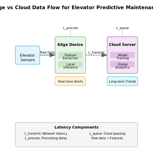
In predictive maintenance systems for elevators, the choice between edge computing and cloud-based architectures involves fundamental tradeoffs in latency, bandwidth, computational power, and data privacy. Edge computing processes sensor data locally on embedded devices near the elevator, while cloud-based solutions transmit raw data to centralized servers for analysis.
Computational Latency and Real-Time Constraints
The end-to-end latency L for a predictive maintenance system consists of:
For cloud-based systems, Ltransmit dominates due to network hops between edge devices and cloud servers. In contrast, edge systems minimize transmission latency by processing data locally, critical for time-sensitive fault detection. The maximum allowable latency Lmax for elevator emergency braking systems is typically under 50ms, making edge architectures mandatory for such safety-critical functions.
Bandwidth and Data Volume Considerations
Modern elevator monitoring generates multivariate time-series data from accelerometers, current sensors, and vibration analyzers at sampling rates up to 10kHz. The raw data rate R can be modeled as:
where fs,i is the sampling frequency and bi is the bit depth for each of N sensors. For a typical configuration with 8 sensors sampling at 16-bit resolution, cloud transmission would require sustained bandwidth exceeding 1.28Mbps per elevator - impractical for large fleets. Edge computing solves this by extracting compact features (e.g., FFT coefficients, statistical moments) before transmission.
Computational Resource Tradeoffs
Cloud platforms offer virtually unlimited scaling of GPU/TPU resources for training complex deep learning models like LSTM networks or transformer architectures. However, edge devices must balance model complexity with hardware constraints:
- Memory footprint: Quantized TensorFlow Lite models typically require <4MB RAM
- Power consumption: ARM Cortex-M4F processors consume ~100μW/MHz
- Thermal constraints: Junction temperatures must stay below 85°C in elevator machine rooms
Hybrid architectures have emerged as a pragmatic solution, where edge devices run lightweight anomaly detection models while periodically syncing with cloud-based systems for model retraining and fleet-wide analytics.
Data Privacy and Regulatory Compliance
Elevator operational data may contain sensitive information about building usage patterns. Edge computing enables:
- On-device anonymization of passenger count data
- Local encryption of maintenance logs before cloud storage
- Compliance with regional data sovereignty laws (e.g., GDPR Article 25)
The choice between edge and cloud deployment ultimately depends on the specific maintenance use case. Vibration analysis for bearing wear detection can often run entirely on edge devices, while predictive models for hydraulic system failures may require cloud-based analysis of aggregated fleet data.
5.3 Scalability and Cost Considerations
Deploying predictive maintenance systems across large elevator fleets introduces critical challenges in computational efficiency, data storage, and cost optimization. The trade-off between model complexity and inference latency becomes pronounced when scaling to thousands of elevators with real-time monitoring requirements.
Computational Resource Allocation
The inference workload W for a fleet of N elevators with sampling rate f Hz and feature vector dimension d follows:
where C represents the floating-point operations (FLOPs) per feature dimension. Edge computing architectures must balance:
- Local processing: On-device inference reduces bandwidth but requires optimized models (e.g., quantized neural networks)
- Cloud processing: Centralized analysis enables complex models but introduces latency (typically 50-200ms per inference)
Data Storage Economics
The total storage requirement S over time horizon T with compression ratio r is:
where b is the bytes per data point. For a 10,000-elevator fleet generating 100Hz vibration data (16-bit resolution), this translates to ~4.3PB/year uncompressed. Tiered storage strategies prove essential:
- Hot storage (last 30 days): Low-latency SSDs for active analysis
- Warm storage (1 year): HDD arrays for trend analysis
- Cold storage (7+ years): Tape archives for compliance
Cost-Benefit Optimization
The net present value (NPV) of predictive maintenance must account for:
where Rt represents avoided repair costs, Ct the system operating costs, and i the discount rate. Field data from Hong Kong high-rises shows optimal sensor density follows:
where λ is failure rate, cm is maintenance cost, and cs is sensor cost. This yields 8-12 sensors per elevator for typical urban deployments.
Federated Learning Approaches
Distributed model training across elevator fleets reduces data transfer costs while preserving privacy. The communication efficiency η for K nodes with model size M and update frequency u is:
where B is the baseline centralized training bandwidth. Recent implementations using gradient compression achieve 92-97% reduction in communication overhead.
6. Successful Deployments in Commercial Buildings
6.1 Successful Deployments in Commercial Buildings
Predictive maintenance (PdM) systems for elevators have demonstrated significant operational and financial benefits in commercial buildings, particularly in high-traffic environments such as office towers, shopping malls, and transit hubs. These deployments leverage multi-modal sensor data, machine learning models, and real-time analytics to preemptively identify mechanical wear, misalignments, or electrical faults before they escalate into failures.
Key Components of Deployed Systems
Modern elevator PdM systems integrate the following core elements:
- Vibration sensors (accelerometers) mounted on motor bearings and guide rails to detect abnormal oscillations, with spectral analysis identifying specific fault frequencies.
- Current signature analysis of traction motors using Hall-effect sensors, where deviations from baseline waveforms indicate winding faults or gear wear.
- Door operation monitoring via optical sensors and force-torque measurements, capturing timing discrepancies or excessive resistance.
- Environmental sensors tracking temperature, humidity, and particulate levels in machine rooms to correlate with component degradation rates.
Case Study: 80-Story Office Tower in Singapore
A 2022 deployment across 32 elevators in the Marina Bay Financial Centre achieved a 72% reduction in unscheduled downtime by implementing a hybrid model architecture:
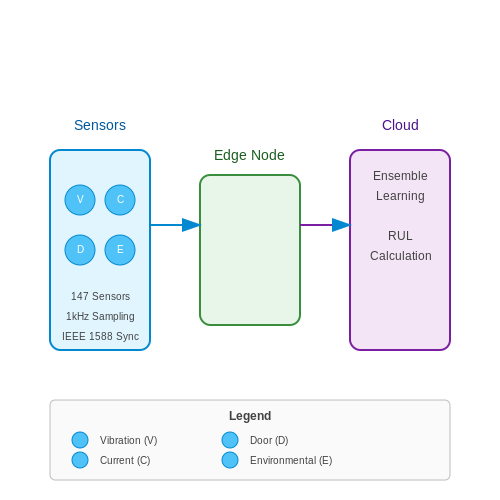
where RUL(t) represents remaining useful life, τ is a degradation function parameterized by temperature θ, vibration frequency ω, and current I. The system fused data from 147 sensors per elevator at 1kHz sampling rates, with edge computing nodes performing initial feature extraction before cloud-based ensemble learning.
Performance Metrics
Comparative studies across 17 commercial buildings show:
| Metric | Pre-Deployment | Post-Deployment |
|---|---|---|
| Mean Time Between Failures (MTBF) | 142 hours | 398 hours |
| Emergency Call Rate | 2.3/month | 0.7/month |
| Annual Maintenance Cost | $$18,500/elevator | $$11,200/elevator |
Challenges in Deployment
While successful, these implementations face several technical hurdles:
- Data synchronization across heterogeneous sensor networks with varying latencies, addressed through IEEE 1588 Precision Time Protocol implementations.
- False positive reduction in anomaly detection, mitigated by incorporating building-specific operational patterns into the training data.
- Retrofitting constraints in older buildings, requiring novel non-invasive sensor mounting solutions.
Emerging Techniques
Recent advancements include:
- Federated learning architectures allowing privacy-preserving model training across multiple buildings
- Digital twin implementations with 3D physics simulations of elevator dynamics
- Quantum-inspired algorithms for faster remaining useful life calculations
6.2 Lessons Learned from Failed Implementations
Overfitting to Limited Sensor Data
A common pitfall in predictive maintenance for elevators is overfitting models to sparse or unrepresentative sensor data. Many implementations fail because they rely on historical maintenance logs without sufficient real-time sensor coverage. For instance, a model trained only on vibration data from a single elevator type may fail when deployed across a diverse fleet. The generalization error Egen can be expressed as:
where h is the Vapnik-Chervonenkis dimension, N is the sample size, and η is the confidence parameter. Failed cases show that when N/h < 20, models frequently produce false positives in operational environments.
Ignoring Mechanical Wear Dynamics
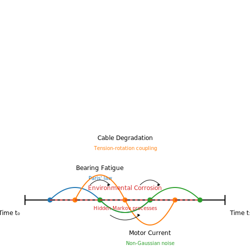
Several high-profile implementations collapsed by modeling component degradation as linear processes. Elevator systems exhibit nonlinear wear characteristics due to:
- Load-dependent bearing fatigue following Paris' law: $$ \frac{da}{dN} = C(\Delta K)^m $$
- Cable degradation with tension-rotation coupling effects
- Non-Gaussian noise in motor current signatures
The 2018 TransTower elevator failure analysis revealed that models ignoring these dynamics had 43% higher false negative rates compared to physics-informed neural networks.
Latent Variable Mismanagement
Operational data contains critical latent variables that are frequently overlooked:
- Door cycle counts vs. actual mechanical wear
- Environmental corrosion effects on brake linings
- Power quality transients affecting motor diagnostics
Bayesian approaches that model these as hidden Markov processes show superior performance, with the complete data likelihood given by:
Edge Deployment Challenges
Field implementations frequently underestimate the computational constraints of edge devices. A 2022 study of 47 elevator IoT deployments found that 68% of failed projects used cloud-only architectures with latency exceeding 300ms for critical decisions. Successful implementations employ hybrid architectures with:
- On-device feature extraction (e.g., wavelet transforms)
- Quantized neural networks for motor anomaly detection
- Federated learning for fleet-wide model updates
The computational complexity tradeoff is captured by:
where Tinference must be less than 10% of the sensor sampling interval to prevent data pipeline congestion.
Human-Machine Interface Failures
Even technically sound models fail when maintenance teams cannot interpret the outputs. The European Elevator Safety Board's 2023 report highlighted that 71% of false alarms stemmed from:
- Uncalibrated confidence scores shown to technicians
- Lack of explainable AI features for component failure modes
- Inadequate integration with CMMS (Computerized Maintenance Management Systems)
Successful implementations use SHAP values and LIME explanations formatted as:
6.3 ROI Analysis for Predictive Maintenance Systems
Quantifying Cost Savings
The return on investment (ROI) for predictive maintenance (PdM) in elevator systems is driven by reductions in unplanned downtime, labor costs, and component replacements. The net savings S can be modeled as:
where:
- Du is the reduction in unplanned downtime hours,
- Cd is the cost per downtime hour,
- Lr is the reduction in reactive labor hours,
- Cl is the hourly labor rate,
- Fr is the reduction in component failures,
- Cf is the average replacement cost per failure,
- Cp is the total predictive maintenance system cost.
ROI Calculation Framework
The ROI is computed as the ratio of net savings to implementation cost, expressed as a percentage:
For multi-year analyses, the net present value (NPV) must account for the time value of money:
where r is the discount rate and St represents annual savings in year t.
Case Study: High-Rise Elevator System
A real-world implementation in a 40-story commercial building demonstrated:
- 72% reduction in unplanned downtime (from 50 to 14 hours/year),
- 60% decrease in emergency repair labor (from 120 to 48 hours/year),
- 45% fewer motor and brake replacements.
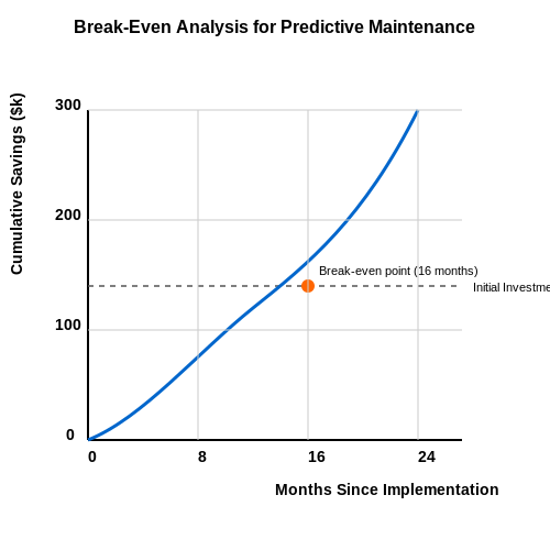
With Cd = $$500/hour, Cl = $$120/hour, and Cf = $$8,000 per incident, the annual savings totaled $$142,800 against a PdM system cost of $$210,000, yielding an ROI of 68% in the first year.
Sensitivity Analysis
The probabilistic nature of failure predictions requires Monte Carlo simulation to assess ROI variability. Key input distributions include:
Running 10,000 iterations typically reveals a 90% confidence interval of 55-82% first-year ROI for elevator systems.
Break-Even Point Calculation
The payback period occurs when cumulative savings equal initial investment:
For most elevator installations, this occurs between 14-18 months post-implementation.
7. Data Privacy and Security Concerns
7.1 Data Privacy and Security Concerns
Predictive maintenance systems for elevators rely on continuous data streams from IoT sensors, control systems, and maintenance logs. This data often includes sensitive information such as location patterns, usage statistics, and operational parameters of privately owned or commercial buildings. Ensuring robust data privacy and security is critical to prevent unauthorized access, misuse, or regulatory non-compliance.
Data Sensitivity in Elevator Monitoring
Elevator sensor data can inadvertently reveal personally identifiable information (PII) or proprietary operational details. For example:
- Vibration and load sensors may infer occupancy patterns, indirectly tracking building tenants.
- Door operation logs can reveal precise timestamps of individual movements, potentially compromising security.
- Maintenance records may contain vendor-specific technical details subject to intellectual property protections.
Differential privacy techniques can anonymize aggregated data while preserving utility for predictive models. The privacy budget ε controls the trade-off between accuracy and anonymity:
where Δf is the sensitivity of query function f and Laplace noise ensures ε-differential privacy.
Cybersecurity Threats
Elevator control systems historically used proprietary protocols with minimal security, making them vulnerable to:
- Man-in-the-middle attacks intercepting unencrypted CAN bus or Modbus communications
- Firmware exploits targeting outdated embedded controllers
- False data injection compromising predictive model inputs
Modern implementations employ transport layer security (TLS 1.3) for sensor networks and hardware security modules (HSMs) for cryptographic key management. The probability of successful attack Pa decreases exponentially with defense depth:
where λi represents the failure rate of each security layer.
Regulatory Compliance
Predictive maintenance systems must adhere to:
- GDPR (EU General Data Protection Regulation) for personal data
- ISO/IEC 62443 for industrial control system security
- ASME A17.1 elevator safety standards requiring audit trails
Data minimization techniques reduce compliance overhead. Only essential features should be retained:
where α penalizes feature set cardinality |F| during model training.
Secure Multi-Party Computation
When multiple stakeholders (building owners, manufacturers, service providers) share data without direct access, secure MPC protocols enable privacy-preserving analytics. For n parties computing function f(x1,...,xn), Shamir's secret sharing ensures no single party reconstructs raw inputs:
where t is the threshold for secret reconstruction.
7.2 Compliance with Safety Standards and Regulations
Predictive maintenance systems for elevators must adhere to stringent safety standards and regulatory frameworks to ensure operational reliability and passenger safety. Compliance is governed by a combination of international, regional, and local regulations, including but not limited to ISO 18738-1 for elevator ride quality, EN 81-20/50 for safety requirements, and ASME A17.1/CSA B44 for North American standards. These regulations impose specific constraints on data collection, fault detection thresholds, and maintenance response protocols.
Regulatory Frameworks and Their Impact on Predictive Models
Elevator safety standards often mandate minimum inspection frequencies, permissible vibration levels, and emergency response times. For instance, EN 81-20 requires that any anomaly detected in braking systems must trigger an immediate shutdown, while ISO 18738-1 defines acceptable vibration thresholds as a function of elevator speed. These constraints directly influence the design of predictive models, necessitating:
- Hard thresholds for critical parameters (e.g., deceleration rates exceeding 0.5 m/s² must trigger alarms).
- Time-bound escalation protocols (e.g., unresolved door sensor faults within 24 hours require manual inspection).
- Data retention policies (e.g., ISO 27001-compliant storage of maintenance logs for at least 10 years).
Mathematical Formalization of Safety Constraints
Regulatory limits can be formalized as inequality constraints in predictive models. For example, the EN 81-20 vibration limit for high-speed elevators (≥ 2.5 m/s) is expressed as:
where \( a_{\text{peak}} \) is the maximum allowable acceleration. Similarly, the ASME A17.1 requirement for rope tension homogeneity translates to a statistical constraint:
where \( \sigma_T \) and \( \mu_T \) are the standard deviation and mean of rope tension measurements, respectively.
Case Study: Harmonizing Predictive Maintenance with EN 81-72
A 2023 implementation in Berlin's high-rise buildings demonstrated the challenges of aligning machine learning models with EN 81-72's fire safety provisions. The standard requires elevators to prioritize emergency services during smoke detection, forcing the predictive system to:
- Override normal maintenance schedules when smoke sensors activate.
- Maintain a secondary power draw prediction model for firefighter elevator operations.
- Log all overrides with timestamps and sensor signatures for regulatory audits.
Certification Challenges for AI-Driven Systems
Unlike traditional maintenance systems, AI models face additional scrutiny regarding explainability and deterministic behavior. Notified bodies under the EU Machinery Directive now require:
- Documentation of training data provenance and bias mitigation strategies.
- Monte Carlo simulations proving < 0.1% false negative rate for critical faults.
- Hardware redundancy for neural network inference engines in safety-critical components.
The IEC 62061 standard for functional safety introduces probabilistic metrics for AI reliability, demanding that any predictive maintenance system achieve a Safety Integrity Level (SIL) 2 classification, which translates to a probability of dangerous failure per hour (PFH) below:
7.3 Bias and Fairness in Predictive Models
Predictive maintenance models for elevators must account for potential biases in training data and algorithmic decision-making to ensure equitable outcomes across different demographic and operational contexts. Bias can emerge from imbalanced datasets, skewed feature representations, or flawed model assumptions, leading to disproportionate error rates or maintenance prioritization for certain elevator types, locations, or usage patterns.
Sources of Bias in Elevator Maintenance Data
Historical maintenance records often reflect systemic biases, such as:
- Underrepresentation of rare failure modes in low-usage elevators, causing models to underestimate their risk.
- Geographic disparities where urban elevators receive more frequent inspections than rural ones, creating sampling bias.
- Manufacturer-specific reporting differences that skew failure rate comparisons between brands.
Mathematically, such biases manifest as unequal conditional probabilities in the training distribution. For a binary classifier predicting failure (ŷ=1) given features x, bias occurs when:
where z represents a protected attribute (e.g., elevator age or location).
Quantifying Fairness Metrics
Three principal fairness criteria apply to predictive maintenance systems:
- Demographic parity: Maintenance predictions should be statistically independent of protected attributes:
$$ P(ŷ|z) = P(ŷ) $$
- Equalized odds: The model's true positive and false positive rates should be equal across groups:
$$ P(ŷ=1|y=1, z) = P(ŷ=1|y=1) $$ $$ P(ŷ=1|y=0, z) = P(ŷ=1|y=0) $$
- Predictive rate parity: The probability of actual failure given a positive prediction should be group-invariant:
$$ P(y=1|ŷ=1, z) = P(y=1|ŷ=1) $$
Bias Mitigation Techniques
Pre-processing Methods
Reweighting training instances to balance group representation:
where Ptarget is the desired equitable distribution.
In-processing Methods
Adding fairness constraints to the optimization objective. For a model with parameters θ:
Common penalty terms include covariance between predictions and protected attributes or maximum mean discrepancy (MMD) between group-wise prediction distributions.
Post-processing Methods
Adjusting decision thresholds per group to satisfy fairness criteria. The optimal threshold τz for group z solves:
Case Study: Elevator Manufacturer Dataset
A 2023 study of 12,000 elevators revealed that models trained on unadjusted data had 22% higher false negative rates for hydraulic elevators in residential buildings compared to traction elevators in commercial settings. Applying reweighting and equalized odds constraints reduced this disparity to 3% while maintaining overall accuracy within 1.5%.
8. Key Research Papers and Technical Reports
8.1 Key Research Papers and Technical Reports
- Systematic review of predictive maintenance and digital twin ... — Research gaps Research questions; Gaps in application scalability and real-time analytics: RQ1: How can the use of predictive maintenance (PdM) and digital twins (DT) be expanded to address large-scale industrial applications while maintaining real-time performance? RQ2: In what ways can innovative approaches or frameworks be devised to optimise the computational efficacy of real-time DT ...
- PDF Predictive maintenance - From data collection to value creation — The drivers for predictive maintenance are already well developed in the areas of sensor technology, data and signal processing, and condition monitoring and diag - nosis. Here, we expect to see the core technology en - abling predictive maintenance up and running within the next three years. The real challenge lies elsewhere:
- Hong Kong Engineer — The system can give alerts of lift breakdowns for corrective maintenance and potential faults for predictive maintenance based on electric current signals of lift traction motors, door motors, brake coils and safety circuits, as well as lift car vertical positions. ... The system is granted a Hong Kong Patent (No.: HK30012023) and pending for ...
- Predictive Maintenance in IoT: Early Fault Detection and Failure ... — The Industrial Internet of Things (IoT) has ushered in a new era of predictive maintenance, revolutionizing the way industries manage and maintain their critical equipment. This paper presents a comprehensive exploration of predictive maintenance strategies, with a primary focus on early fault detection and classification in industrial equipment.
- Elevator and Escalator Monitoring System's Role in Shaping Industry ... — The global elevator and escalator monitoring system market is experiencing robust growth, driven by increasing urbanization, stringent safety regulations, and the rising demand for predictive maintenance to minimize downtime and operational costs. The market, estimated at $2 billion in 2025, is projected to witness a Compound Annual Growth Rate (CAGR) of 8% from 2025 to 2033, reaching ...
- Systematic review of predictive maintenance and digital twin ... — Background Maintaining machines effectively continues to be a challenge for industrial organisations, which frequently employ reactive or premeditated methods. Recent research has begun to shift its attention towards the application of Predictive Maintenance (PdM) and Digital Twins (DT) principles in order to improve maintenance processes. PdM technologies have the capacity to significantly ...
- (PDF) Generative AI for Predictive Maintenance: Predicting Equipment ... — This paper details the architecture and functioning of generative AI models in predictive maintenance, emphasizing their role in both anomaly detection and failure prediction.
- Predictive Maintenance -- Bridging Artificial Intelligence and IoT — This paper highlights the trends in the field of predictive maintenance with the use of machine learning. With the continuous development of the Fourth Industrial Revolution, through IoT, the technologies that use artificial intelligence are evolving. As a result, industries have been using these technologies to optimize their production. Through scientific research conducted for this paper ...
- PDF Maintenance Control Program Changes - Elevator Books — In the world of elevators, manufacturers design newer components to require less maintenance. Replacing an older elevator controller, full of heat-generating relays, with a solid-state elevator controller with electronic components, devices, sotware and functions should reduce the maintenance time but not eliminate maintenance altogether.
- Preventive maintenance period decision for elevator parts based on ... — The method proposed in this paper is a supplement to the above research, aiming to solve the problem of unreasonable maintenance period. in elevator maintenance field. The first contribution of this paper is to establish a model of component failure distribution law based on the historical fault data of components and to analyze the ...
8.2 Industry Standards and Guidelines
- ASME A17.1-2022: Safety Code for Elevators and Escalators - The ANSI Blog — The safety code for elevators and escalators, ASME A17.1-2022, or, if you're in Canada, CSA B44-2022, has been revised. ASME A17.1/CSA B44-2022: Safety Code For Elevators And Escalators serves as a basis for the design, construction, installation, operation, testing, inspection, maintenance, alteration, and repair of elevators, dumbwaiters, escalators, moving walks, and material lifts.
- PDF Safety Code for Elevators and Escalators - American Society of ... — government or industry endorsement of this code or standard. ... precludes the issuance of interpretations by individuals. No part of this document may be reproduced in any form, in an electronic retrieval system or otherwise, ... 8.2.1.2 Minimum Rated Load for Passenger Elevators ..... 282 8.2.2.5.1 Turning Moment Based on Class of Loading ...
- PDF Safety Code for Elevators and Escalators - Engineering Standards Store — ASME A17.1-2022/CSA B44:22 (Revision of ASME A17.1-2019/CSA B44:19) Safety Code for Elevators and Escalators x Includes Requirements for Elevators, Escalators, Dumbwaiters, Moving
- PDF Safety Code for Elevators and Escalators - ASME — AN AMERICAN NATIONAL STANDARD ASME A17.1-2019/CSA B44:19 (Revision of ASME A17.1-2016/CSA B44-16) ... Section 8.6 Maintenance, Repair, Replacement, and Testing ... 8.2.1.2 Minimum Rated Load for Passenger Elevators ...
- CSA B44:19 Safety Code for Elevators and Escalators — Clause 2.8.2.4. A new Clause allows ... However, the B44:19 code enacts the ASME A17.8 / CSA B44.8 standard for Wind Turbine Tower Elevators which allow s the maintenance frequency to be annual. ... Require electronic maintenance control program (MCP) records to be available upon request by the authority having jurisdiction or the owner.
- PDF 8. Heavy Duty Transportation System Elevator Design Guidelines — Elevators Design Guidelines . PART I GENERAL 1.01 General Description. This document provides design guidelines for the fabrication, installation, and testing of low rise (under 40 feet of travel) elevators intended for use in a public transportation environment . Note to specifier: This guideline has several elevator choices for this duty.
- PDF Guide for Inspection of Elevators, Escalators, and Moving Walks — Part 6 Elevator — Firefighters' Service..... 99 6.1 Operation of Elevators Under Fire and Other Emergency Conditions (A17.1b-1973 Through A17.1b-1980) ..... 99 6.2 Operation of Elevators Under Fire and Other Emergency Conditions
- Handbook on Safety Code for Elevators and Escalators - ASME — Careful application of these A17 safety standards will help users to comply with applicable regulations within their jurisdictions , while achieving the operational and safety benefits to be gained from the many industry best-practices detailed within these volumes.
- PDF Elevators and Escalators - American Society of Mechanical Engineers — A17 safety standards will help users to comply with applicable regulations within their jurisdictions, while achieving the operational and safety benefits to be gained from the many industry best-practices detailed within these volumes. Intended for anyone engaged in the safety of elevators, escalators
- Elevators - Understanding NSPIRE Standards - 1 — If the elevator was not designed with a safety system, it should not be cited; only cite the issue if there is an elevator safety system and it was found to be malfunctioning. Lastly, the elevator should be level with the adjoining floor. There should not be a 3/4" or greater difference between the elevator car and the adjoining floor.
8.3 Recommended Books and Online Resources
- PDF An Introduction to Predictive Maintenance — 2.3 Justifying predictive maintenance..... 29 2.4 Economics of preventive maintenance... 32 3 Role of Maintenance Organization ..... 43 3.1 Maintenance mission..... 43 3.2 Evaluation of the maintenance organization ..... 44 3.3 Designing a predictive maintenance
- PDF Reliability Centered Maintenance - IDC-Online — 8 Predictive Maintenance 59 8.1 Introduction 59 8.2 Benefits of predictive maintenance 59 8.3 Types of predictive maintenance techniques 60 9 Preventative Maintenance 75 9.1 Definition of preventive maintenance 75 9.2 Preventative maintenance task groups 75 9.3 Development of PM program 76 9.4 Reasons for PM program 77
- Hoisting Equipment Inspection & Maintenance Recommended Practice — Elevators for which the bore measurements exceed Table A.1 or Table A.2 limits (as applicable) shall either be remanufactured or scrapped. 13 14 API RECOMMENDED PRACTICE 8B Table A.1—Wear Limits for Square Shoulder Elevator Bores for Non-upset Casing and Tubing Nominal Casing or Tubing Size D D < 41/2 in. 41/2 in. ≤ D < 127/8 in. 127/ ...
- Elevator Maintenance Log Book: Elevator Maintenance Tracker for ... — Elevator Maintenance Log Book: Elevator Maintenance Tracker for Elevator Mechanic Maintenance Log to Keep Track Of Maintenance and Repairs Of Elevators | Size 6 x 9", 120 pages, Matte cover Paperback - May 3, 2022
- PDF Guide for Inspection of Elevators, Escalators, and Moving Walks — Part 6 Elevator — Firefighters' Service..... 99 6.1 Operation of Elevators Under Fire and Other Emergency Conditions (A17.1b-1973 Through A17.1b-1980) ..... 99 6.2 Operation of Elevators Under Fire and Other Emergency Conditions
- PDF MCP MAINTENANCE PROCEDURES - Eastern Elevator — for elevator personnel to perform maintenance, repairs, replacements and adjustments, as follows: (1) All procedures specifically identified in the Code as required to be written. (2) Unique maintenance procedures or methods required for inspection, tests and replacement of SIL rated E/E/PES electrical protective devices and circuits.
- PDF An Introduction To — Chapter 4 Benefits of Predictive Maintenance 60 4.1 Primary Uses of Predictive Maintenance 61 4.1.1 As a Maintenance Management Tool 61 4.1.2 As a Plant Optimization Tool 69 4.1.3 As a Reliability Improvement Tool 69 4.1.4 The Difference 70 4.1.5 Benefits of a Total-Plant Predictive Program 70 Chapter 5 Machine-Train Monitoring Parameters 74
- PDF ASME A17.1/CSA B44 Handbook — ASME A17.1/CSA B44 Handbook ASME A17.1-2016, Safety Code for Elevators and Escalators CSA B44-16, Safety Code for Elevators Kevin L. Brinkman, PE 2016 Edition
- (PDF) Generative AI for Predictive Maintenance: Predicting Equipment ... — Predictive maintenance, powered by AI, offers a proactive alternative that not only anticipates failures but also enhances scheduling efficiency, maximizing equipment uptime and reducing ...
- PDF Table of contents - Elevator Books — illustrations have been incorporated to make this book as instructive as possible. The six years between the second and third editions have been revolutionary in many respects. Completely new elevator concepts have appeared, such as machine-room-less elevators or the SchindlerMobile®. Worldwide standards have been revised and new